Predicting ecological regime shift under climate change : new modelling and molecular based approaches

Received Jan.30, 2013; accepted May 2, 2013.

∗ Corresponding author. E-mail: [email protected] © 2013 Current Zoology

Predicting ecological regime shift under climate change:

New modelling techniques and potential of molecular-based

approaches

Richard STAFFORD

, V. Anne SMITH

, Dirk HUSMEIER

, Thomas GRIMA

,

Barbara-ann GUINN

1_{School of Applied Sciences, Bournemouth University, BH12 5BB, UK} 2_{School of Biology, University of St Andrews, St Andrews, KY16 9ST, UK} 3_{School of Mathematics and Statistics, University of Glasgow, G12 8QW, UK} 4_{Department of Life Sciences, University of Bedfordshire, LU1 3JU, UK}

Abstract Ecological regime shift is the rapid transition from one stable community structure to another, often ecologically infe-rior, stable community. Such regime shifts are especially common in shallow marine communities, such as the transition of kelp forests to algal turfs that harbour far lower biodiversity. Stable regimes in communities are a result of balanced interactions be-tween species, and predicting new regimes therefore requires an evaluation of new species interactions, as well as the resilience of the ‘stable’ position. While computational optimisation techniques can predict new potential regimes, predicting the most likely community state of the various options produced is currently educated guess work. In this study we integrate a stable regime op-timisation approach with a Bayesian network used to infer prior knowledge of the likely stress of climate change (or, in practice, any other disturbance) on each component species of a representative rocky shore community model. Combining the results, by calculating the product of the match between resilient computational predictions and the posterior probabilities of the Bayesian network, gives a refined set of model predictors, and demonstrates the use of the process in determining community changes, as might occur through processes such as climate change. To inform Bayesian priors, we conduct a review of molecular approaches applied to the analysis of the transcriptome of rocky shore organisms, and show how such an approach could be linked to meas-ureable stress variables in the field. Hence species-specific microarrays could be designed as biomarkers of in situ stress, and used to inform predictive modelling approaches such as those described here [Current Zoology 59 (3): 403–417, 2013].

Key Words Regime shift, Phase shift, Alternative stable state, Intertidal, Food web, Resilience

While the net, global effect of anthropogenic climate change on physical properties such as temperature are well documented in scientific literature (Peters and Lovejoy, 1994; IPCC, 2007), the magnitude of these effects are less certain, and the local effects are less cer-tain still, and most likely spatially and temporally vari-able (Peters and Lovejoy, 1994; Gilman et al., 2010). Given the uncertainty of changes to physical environ-ments, changes in biological characteristics of ecologi-cal communities are highly uncertain and current mod-elling approaches closely match biological distributions to the physical predictions, with little regard for other biological processes such as species interactions (e.g. climate envelope modelling-Pearson and Dawson, 2003; Gilman et al., 2010).

Physiological changes to climate-induced stressors,

such as temperature, have been conducted for many species. In invertebrates, studies such as lethal tempera-ture, heat coma temperatures or changes to heart rate in response to increasing temperatures have been con-ducted on many species, both in the laboratory, and in field conditions (reviewed by Somero, 2002). However, the wealth of possible data given by modern genomic techniques, such as studying gene expression using mi-croarrays, has generally been confined to the laboratory (Kammenga et al., 2007; van Straalen and Roelofs, 2012). While the lack of knowledge of gene function hinders field-based studies on most invertebrates (van Straalen and Roelofs, 2012), examining changes along stress gradients (i.e. latitudes) gives an indication of how overall levels of gene expression may vary in situ

2008). Determining such changes in gene expression in measurably significantly different microhabitats would therefore provide a mechanism of predicting sub-lethal physiological stress caused by climate-induced factors, such as temperature, or indeed, any other physiological stress. Such investigations could predict which species may suffer most from any changes.

Given any species exists as part of an ecological community, interacting with prey, predators, parasites and competitors, changes in the physiology, ecology or distribution of any species will have some degree of community level effect. Predicting changes in commu-nities, and resultant changes to ecosystem services, is therefore a complex task (Peters and Lovejoy, 1994). Shallow marine ecosystems are well studied, and ecolo- gically and economically important (Peterson and Lubchenco, 1997). For example, many shallow marine ecosystems contain economically important fish species, either directly, or as juveniles in nursery grounds. Fur-thermore, subtidal reefs, such as kelp forests and coral reefs are important to tourism, through SCUBA diving (Peterson and Lubchenco, 1997). These ecosystems also are some of the most threatened by climate change, with rising temperatures being attributed to aspects of coral bleaching and kelp death (e.g. Mumby, 2007).

Many shallow marine and intertidal ecosystems demonstrate alternative regimes or ecological stable states (Lewontin,1969; Sutherland, 1974; May, 1977; Harrold and Reed, 1985; Knolton, 1992; Konar and Es-tes, 2003; Petraitis and Dudgeon, 2004; Mumby, 2007), where communities are robust to small perturbations and disturbances, and population sizes are relatively stable, (although seasonal cycles can occur in some in-stances). Large disturbances, however, create rapid ‘re-gime shifts’, for example, the reduction of high diversity kelp forest to largely barren algal turf (Harrold and Reed, 1985; Konar and Estes, 2003). In general, post re-gime-shift states are not only highly stable themselves, but, compared to pre-regime shift states, are also ‘poorer’ both in biodiversity and provision of ecosystem services (Walker and Salt, 2006). Recently an examina-tion of these rapid changes by Dudgeon et al. (2010) has suggested the use of the term ‘alternative stable state’ for where two or more possible stable community structures exist with the same physical environment (e.g. temperature), and ‘phase’ or ‘regime shift’ to be used where only one community exists at a given level of environmental variables (such as temperature). This means an invasive species may create a new alternative stable state, where as a disturbance such as climate

change increasing temperatures will create a new re-gime. Both systems, however, rely on positive feedback to keep communities stable until a ‘tipping point’ occurs (Dudgeon et al., 2010). The methods used in this study apply equally to both classifications; however, since the technique depends on the concept of stability of commu-nities, we have used the term ‘stable state’ throughout.

With some degree of knowledge about current spe-cies interaction strengths in the community and given the robustness of community structure when in a stable state, it is possible to build and parameterise stable state models, based on localised computational search strate-gies (Stafford et al., 2008). Briefly, these involve searching multidimensional space for optima, as per many existing computational optimisation techniques such as genetic or evolutionary algorithms (e.g. Holland, 1992). However, in this situation it is necessary to find local optima, rather than the global optimum value – a much computationally simpler process. Equally, given a known disturbance to any one or multiple species in the community, it is possible to apply similar stochastic localised optimisation techniques to predict new poten-tial stable states or regimes (Stafford et al., 2008). Hence, although we apply this technique under the con-text of climate change, it is equally applicable to any disturbance event that affects population sizes or inter-actions between species.

ex-pression data may inform of relative in situ stress levels (see previously).

This study builds on the concepts developed in Staf-ford et al. (2008) for predicting new stable states, and applies the results to a ‘typical’ rocky shore community as could be affected by climate change (but in practice, affected by any community or population level distur-bance). It considers a much more complex community than previously examined, which is likely to result in a far greater number of post regime-shift stable states. As such, community resilience and Bayesian belief net-works are used to inform decisions on post regime-shift community structure. Although very much preliminary work, we also review studies on differential gene ex-pression of rocky shore organisms from different mi-crohabitats, and examine how these data could be in-corporated into these predictive models.

1 Materials and Methods

1.1 Rocky shore model

Rocky shores are coastal marine ecosystems, which show stable or seasonally stable community structure, exhibiting several different stable states depending on physical or biological properties (e.g. Petraitis and Dudgeon, 1999; 2004). They are extensively studied in terms of their ecology, with many in situ experiments having been conducted to determine grazing, predation and competitive interactions between species (reviewed by Little et al., 2009). For the purposes of this study, a sim-plified version of a rocky shore community is extracted from what commonly exists in the UK. Grazing, competi-tive and predatory interactions are all included. The rocky shore model should be considered representative of a real rocky shore community, but not wholly accurate in every detail. As such, results should be considered as indicative of what may occur through climate change, rather than true predictions. The reasons for this approximate model, rather than an exact simulation, are due to the data requirements of the model, and further research to make the approach predictive is given in the discussion.

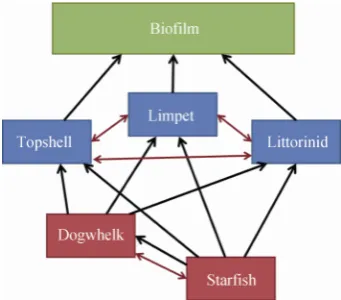
The rocky shore model considers three species of grazing gastropod, which graze on epilithic photosyn-thetic biofilm. Due to their larger size, limpets are the competitively superior gastropod on the mid shore of many rocky shore ecosystems, but co-exist alongside grazing topshells and littorinids (Fig. 1). Competition occurs between all of these three species. Predatory in-teractions occur from both dogwhelks, a predatory gas-tropod mollusc, and starfish. Some degree of

competi-tion occurs between these species, but starfish will also prey on dogwhelks (Fig. 1).

Fig. 1 Community interaction web, showing tropic inter-actions between species in black (arrow points from predator to prey) and competitive interactions in red

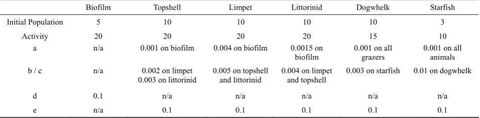
A series of equations are used to realise the rocky shore model in R (R core development team, 2012). At each timestep of the model, grazing/predatory in-teractions occur, competitive inin-teractions occur and growth of the population (through recruitment) occurs. Each of these types of interaction is simulated by the following equations, where initial values for popula-tion, activity and constants for each species are given in Table 1.

Grazing and predation, of species X on species Y: PredX→Y = a . Activityx . Populationx . Populationy,

where activity relates to the time spent active on the shore during a tidal cycle, and a is the predation coefficient.

Competition between species X and species Y: CompX↔Y=b. Populationx. Activityx. c. Populationy.

Activityy,

where b is the competition coefficient of species Y, and c is the competition coefficient of species X.

Growth of biofilm:

Growthbiofilm = d . Populationbiofilm . Activitybiofilm,

where d is a growth coefficient, activity relates to the time spent active on the shore during a tidal cycle, and population is a measure of biofilm density.

Growth of Animals: Growthx = e . ΣPredx,

where all the predatory or grazing interactions for a single species are summed.

Change in population of species X:

Population x,t+1 = Population x,t + Growthx - ΣCompx -

Table 1 Initial parameters of the model used in the mathematical equations

Biofilm Topshell Limpet Littorinid Dogwhelk Starfish

Initial Population 5 10 10 10 10 3

Activity 20 20 20 20 15 10

a n/a 0.001 on biofilm 0.004 on biofilm 0.0015 on

biofilm 0.001 on all grazers 0.001 on all animals b / c n/a 0.002 on limpet

0.003 on littorinid 0.005 on topshell and littorinid 0.004 on limpet and topshell 0.003 on starfish 0.01 on dogwhelk

d 0.1 n/a n/a n/a n/a n/a

e n/a 0.1 0.1 0.1 0.1 0.1

Population figures relate to relative biomass of organisms – but are indicative figures, rather than exact measurements from real shores, and hence no units are given.

Where the sum of predatory interactions on species X and competitive interactions involving species X are subtracted from the growth.

The simulation runs for 10 timesteps, and the stabil-ity of the system is determined by summing the per-centage change of the population of each species be-tween the first and last timestep. Ten timesteps were used as preliminary results showed that systems stable for this length of time remained stable for much longer periods. Given the high computational demands of op-timisation (multiple individuals over multiple genera-tions, replicated multiple times – see below), reducing the number of timesteps in the model resulted in much faster optimisation and performance of the technique.

1.2 Parameterisation and optimisation of the rocky shore model

The rocky shore model above was parameterised with best guess estimates. For example, competition coefficients were generated relative to each other, based on prior experimental knowledge (Table 1). Population sizes were again based on limited prior knowledge of biomass or energetic turnover of the species in question. However, as detailed previously, the parameters are in-dicative, rather than representing any definite quantity of the actual system. Over 10 timesteps, several popula-tions became extinct, hence the model did not represent a stable state. To parameterise the rocky shore model into a stable state, a form of evolutionary algorithm was used, deliberately designed to find localised optima, rather than the normal goal of finding global optima. Note, the evolutionary algorithm is simply an optimisa-tion technique used on the identified populaoptimisa-tion sizes and interaction parameters, and does not imply evolu-tion or adapevolu-tion of individuals or populaevolu-tions of rocky shore organisms in any way.

Briefly, the algorithm generated an initial 120 pa-rameter sets (or in terms of evolutionary algorithms, a population of 120 individuals), with values for each of

the parameters in table 1, uniformly randomly generated in the range X±(X/3), where X is the value in table 1.

Each ‘individual’ set of parameters is evaluated over 10 timesteps described above, and the stability of the system (or ‘fitness’ of the individual) is determined by summing the percentage change of the population of each species between the first and last timestep. The best eight individuals (those with the lowest level of change in population sizes, representing the ‘fittest’ in-dividuals in the population) were then copied without any modification in the population in the next genera-tion, and 14 copies of each of these eight individuals were made, with modification, which is ± 10% of the current value. This evolutionary algorithm is run for 100 generations, to minimise changes in the population of each species, and the best ‘individual’ or set of parame-ters selected at the end, to provide parameparame-ters which create a more stable system, but still bear resemblance to the initial parameter set. ‘Individuals’ or parameter sets were only considered stable positions if the overall change in the population of all species (the selected ‘fitness’ parameter above) was < 10% (or an average change per species < 1.7%).

1.3 Possible community change scenarios for most sensitive species

Table 2 Scenarios of possible species responses to climate change, used to determine new stable states

Species 1 Species 2 Species 3

Scenario 1 Limpet population reduction by 35% - -

Scenario 2 Starfish population reduction by 50%

Scenario 3 Starfish population reduction by 50% Limpet population reduction by 35% Biofilm population increased by 30 %

scenarios where information on only a single species is known and a more complex scenario, where effects on multiple species are known from prior evidence (e.g. ex-perimental or observational data). However, mainly these are illustrative accounts to understand the dynamics of the rocky shore model, rather than based on knowledge of likely species tolerances to climate change. As such, it is entirely possible that in reality, different changes may occur, or that these changes could arise as a result of a different disturbance (for example disease in starfish).

1.4 Bayesian belief network

A Bayesian belief network was constructed using JavaBayes (Cozman, 2001). Essentially, each species in a community is considered as a node in the belief net-work graph. Each species can either be ‘increasing’ or ‘decreasing’ in population size. Although in theory other levels can be incorporated into such networks (i.e. in-creasing a lot, inin-creasing a little, not changing), this simple two level approach reduces the level of ‘prior knowledge’ required from the system, and is commonly used in other belief network studies in ecology (e.g. Hammond and Ellis, 2002).

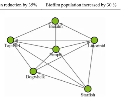
Bayesian networks are directed acyclic graphs (DAGs). This is consistent with trophic interactions, due to the fact that the effect of the predator on the prey (death) is much stronger than the reverse effect (providing food), and the assumption of directed in-teractions is thus appropriate. However, the DAG as-sumption is too restrictive for modelling competition, given that these interactions are intrinsically bidirec-tional. For example, there is a competitive interaction between limpets and topshells, and since limpets are considered the dominant competitor, there is no recip-rocal competition from topshells on limpets indicated in the Bayesian network (Fig. 2). To overcome this issue, the species classed as the superior competitor (i.e. limpets over topshells and littorinids, and lit-torinids over topshells) is shown to have an effect on the inferior competitor, but reciprocal competition is considered only when assigning ‘prior’ values to the interaction (see example below).

Each node or species has a probability computed from prior knowledge of the network or community, and

Fig. 2 Bayesian belief network structure, note one way competitive interactions, and only a single link between starfish and dogwhelk

observations on the individual species that comprise the network or community (i.e. known changes to species – summarised in Table 2). For example, the most complex node is probably that of ‘Topshell’ where the probability of the population increasing or decreasing depends on all other animals in the system, either through competi-tive or trophic interactions, more formally:

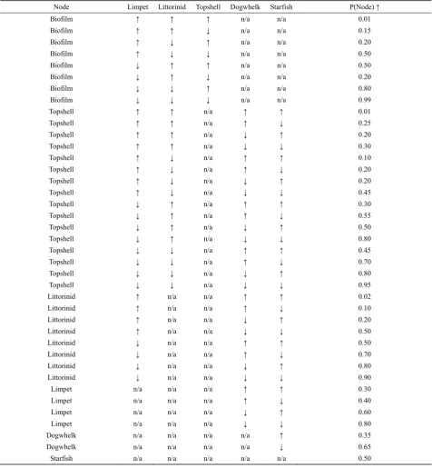
P (Topshell | Limpet, Littorinid, Starfish, Dogwhelk), Priors for each of the nodes are based on best guess approaches from known interactions (Table 3). Reciprocal competition is considered in these ap-proaches. For example, the effects of predation on limpets are much less certain than for some of the other grazing species, because when predation fa-vours the other species (e.g. littorinids or topshells – or possibly dogwhelks), then the limpets may in-crease in population size, despite the inin-crease in predators, due to competitive effects.

Observations are then made on actual species de-creases and inde-creases, as per Table 2, where increase in growth or decrease in activity are defined as ‘increase’ or ‘decrease’ respectively. Observations therefore have known levels of probability, and are either certainly increasing (pdecrease = 0, pincrease = 1) or certainly

decreas-ing (pdecrease = 1, pincrease = 0).

1.5 Combining the results of each model

Table 3 Prior values for the Bayesian belief network

Node Limpet Littorinid Topshell Dogwhelk Starfish P(Node) ↑

Biofilm ↑ ↑ ↑ n/a n/a 0.01

Biofilm ↑ ↑ ↓ n/a n/a 0.15

Biofilm ↑ ↓ ↑ n/a n/a 0.20

Biofilm ↑ ↓ ↓ n/a n/a 0.50

Biofilm ↓ ↑ ↑ n/a n/a 0.50

Biofilm ↓ ↑ ↓ n/a n/a 0.20

Biofilm ↓ ↓ ↑ n/a n/a 0.80

Biofilm ↓ ↓ ↓ n/a n/a 0.99

Topshell ↑ ↑ n/a ↑ ↑ 0.01

Topshell ↑ ↑ n/a ↑ ↓ 0.25

Topshell ↑ ↑ n/a ↓ ↑ 0.20

Topshell ↑ ↑ n/a ↓ ↓ 0.30

Topshell ↑ ↓ n/a ↑ ↑ 0.10

Topshell ↑ ↓ n/a ↑ ↓ 0.20

Topshell ↑ ↓ n/a ↓ ↑ 0.20

Topshell ↑ ↓ n/a ↓ ↓ 0.45

Topshell ↓ ↑ n/a ↑ ↑ 0.30

Topshell ↓ ↑ n/a ↑ ↓ 0.55

Topshell ↓ ↑ n/a ↓ ↑ 0.50

Topshell ↓ ↑ n/a ↓ ↓ 0.80

Topshell ↓ ↓ n/a ↑ ↑ 0.45

Topshell ↓ ↓ n/a ↑ ↓ 0.70

Topshell ↓ ↓ n/a ↓ ↑ 0.80

Topshell ↓ ↓ n/a ↓ ↓ 0.95

Littorinid ↑ n/a n/a ↑ ↑ 0.02

Littorinid ↑ n/a n/a ↑ ↓ 0.10

Littorinid ↑ n/a n/a ↓ ↑ 0.20

Littorinid ↑ n/a n/a ↓ ↓ 0.50

Littorinid ↓ n/a n/a ↑ ↑ 0.50

Littorinid ↓ n/a n/a ↑ ↓ 0.70

Littorinid ↓ n/a n/a ↓ ↑ 0.80

Littorinid ↓ n/a n/a ↓ ↓ 0.90

Limpet n/a n/a n/a ↑ ↑ 0.30

Limpet n/a n/a n/a ↑ ↓ 0.40

Limpet n/a n/a n/a ↓ ↑ 0.60

Limpet n/a n/a n/a ↓ ↓ 0.80

Dogwhelk n/a n/a n/a n/a ↑ 0.35

Dogwhelk n/a n/a n/a n/a ↓ 0.65

Starfish n/a n/a n/a n/a n/a 0.50

The final column gives the probability of the named node increasing in size of population, given the increases or decreases shown.

new stable community states. The computational opti-misation approach provides a unique combination of population sizes and parameters for each run of the process (in this case, the process is run 100 times, so 100 predictions are produced). To assess resilient stable states, we use a simple clustering dendrogram on stan-dardised values of the different population sizes of the six species considered. Specifically, we use the ’hclust’ function in R, on the standardised distance matrix cal-culated using the ‘daisy’ function in the ‘cluster’ library

predic-tion. Only when five or more possible post disturbance communities fell within a cluster were they considered a resilient community, as the stable states should be able to slightly change parameter settings and remain stable. As such, one potential stable state from each cluster was identified as a ‘typical’ representation of this state which was one of the pair with the closest distance between them.

The population size values for individuals from within each cluster were compared with the predictions of the Bayesian network. For example, where the Bayesian network indicated that the population of a species was likely to increase with a probability of 0.7, for a given scenario, the possible stable states were exa- mined, and a value of 0.7 given for that species if the value had increased from the baseline population and 0.3 if it has decreased from the baseline population. The overall likelihood of the newly parameterised rocky shore model, based on the Bayesian network predictions, was calculated as the product of all six species predic-tions, and the highest overall value was considered the best fit with the Bayesian network, this value is pre-sented in the results as the ‘product of probabilities’.

1.6 Determining significant differences in in situ

stress in marine molluscs in different microhabitats

Determination of in situ stress in relation to tempera-ture, desiccation and biological factors such as competi-tion may provide a species specific set of biomarkers to inform of sub-lethal effects in organisms. Hence, once biomarkers are identified, examining them in other in-dividuals may inform of in situ stress acting on organ-isms and provide a mechanism for determining likely future response to this stress, even at a very basic level such as determining whether the population is likely to decrease if conditions provide more stress to that spe-cies than to others. As such, molecular responses, such as gene expression, known to be linked to stress (rather than knowledge of the exact role of the gene), can be used to inform predictive models, especially simple to parameterise models such as Bayesian networks – where high levels of stress can be used to make ‘obser-vations’ on particular populations (i.e. they are likely to decrease).

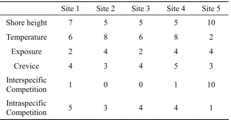
A first stage of this process is to determine if bio-markers can be linked to significantly different micro-habitats in terms of levels of stress. To determine if sig-nificant differences in microhabitats exist for a marine mollusc, Littorina saxatilis were examined on man- made breakwaters at Rottingdean Beach (50.80169° N, 0.05636° W) in Sussex, in August 2012. A number of parameters were collected on physical and biological

conditions at the three collection sites on the beach con-sisting of two sides of a rock breakwater (site 1 and 2), and two sites on a concrete jetty approximately~200m away from the other sites (sites 3 and 4, Table 4). To facilitate comparison with other microhabitats where the species is known to occur, the site was also compared to data collected from Hartlepool (County Durham UK, 54.69907 °N, 1.17751 °E , Site 5) as part of a separate study (Stafford, 2002).

These conditions were then compared to a previous comprehensive study on Littorina saxatlis distribution (Stafford, 2002) to produce a 1–10 marking scheme for each of the characteristics (Table 5), where 1 repre-sented a low value of a parameter and 10 a value close to the maximum recorded over a wide range of shores in the UK.

To calculate the weighted values, the following as-sumptions were used:

1) Typical exposure from wave action was calculated from data of historic swell height averaged over all months of the year (1.3 m in Sussex and 1.35 m in County Durham). This was compared to data from the Outer Hebrides, demonstrating the most exposed loca-tion and largest average swell height (3.1 m) in the UK (data from MetCentral Ltd).

Table 4 Characteristics of the sites from where Littorina saxatilis were collected

Site 1 Site 2 Site 3 Site 4 Site 5

Shore height

(+ C.D) (m) 8.3 6.3 6.2 6.3 12.3

L. saxatilis density

(m2₎ 130 90 110 120 20

M. neritoides

density (m2₎ 55 0 0 25 860

% crevice 8 6 8 10 6

Aspect E W E W NE

Mean aggregation size (n, both species

combined)

17 4 2 4 45

Table 5 Adjusted characteristics of Littorina saxatilis for each location

Site 1 Site 2 Site 3 Site 4 Site 5

Shore height 7 5 5 5 10

Temperature 6 8 6 8 2

Exposure 2 4 2 4 4

Crevice 4 3 4 5 3 Interspecific

Competition 1 0 0 1 10

Intraspecific

2) For south coast (Sussex) location the predominant wind and swell direction is SW. Therefore a reduction of 40% in exposure was used for the site facing SE, which was also consistent with observations on breaking wave height at the locations. NE is the predominant swell direction in County Durham, so no adjustment was made for site 5.

3) The south-east of England (Sussex) was shown to have an average annual temperature of 7°C compared to a coastal maximum average of 8°C (Cornwall) and minimum of 3°C (N.E. Scotland) in the UK (data from metoffice.gov.uk), County Durham had average annual temperatures of 5°C.

4) Heat absorption (and hence rock temperature) of east facing walls is 20% lower than that of west facing walls, based on data from previous studies (Nakamura and Oke, 1967). In this case, northeast facing walls were conservatively considered the same as east facing walls.

5) Maximum density of Littorina saxatilis and Me-larharphe neritoides combined can be as high as 900m-2_.

Maximum density of Littorina saxatilis was 300 m-2

(Stafford, 2002).

6) Maximum recorded shore height of each species >

12 m +C.D. (Stafford, 2002).

7) Maximum crevice density is ~ 20 % of the rock surface (Stafford, 2002).

For each site the percentage contribution of each factor (e.g. shore height) was calculated. These per-centages were used in a bootstrapped Principal Compo-nent Analysis (following the procedure in Stafford et al., 2012a) to determine significant differences in micro-habitat between sites.

2 Results

2.1 Bayesian belief network

Initially, the Bayesian belief network was altered us-ing ‘observations’ of what was predicted to happen to individual species, or groups of species, as a result of climate change (as per Table 2). Specific increases or decreases were applied for these ‘observed’ species nodes (posterior probabilities for increases in population size set at 0 for limpets and starfish in scenarios 1 and 2 respectively, and 0, 0 and 1 for increases to limpets, starfish and biofilm respectively for scenario 3) and the resultant changes in posterior probability for the unob-served species are given in Table 6.

Table 6 Results of scenarios of Bayesian belief network – data are for posterior probabilities of a given node increasing (given observations on population sizes of certain species in the community), values in bold indicate ‘observed’ values set at either 1 (increasing) or 0 (decreasing)

Biofilm Topshell Littorinid Limpet Dogwhelk Starfish

Control 0.43 0.39 0.46 0.52 0.5 0.5

Scenario 1 0.51 0.54 0.69 0 0.66 0.52

Scenario 2 0.41 0.45 0.50 0.54 0.65 0

Scenario 3 1 0.73 0.55 0 0.86 0

2.2 Parameterisation and optimisation of the rocky shore model

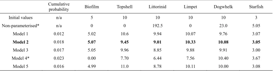
The initial rocky shore model and parameters pre-sented in Table 1 did not produce a stable state model, but a model where populations of biofilm, topshells and limpets collapsed, and littorinid and dogwhelk populations increased dramatically over 10 timesteps (Table 7). Parameterisation of the rocky shore model (using the local optimisation process described previ-ously) to find a stable state model, similar to the initial model produced a range of similar models (examples in Table 7). The Bayesian network also predicted changes to population sizes for the initial ‘control’ population, and the rocky shore model with best fit from the Bayesian network (the highest product of probabilities) was chosen as model 2, below. Techni-cally, model 4 had a higher product of probability, but

Table 7 Results of optimisation runs for initial parameterisation. Fitness values and population sizes given after 100 gen-erations of selection of 10 cycles of the model

Cumulative

probability Biofilm Topshell Littorinid Limpet Dogwhelk Starfish

Initial values n/a 5 10 10 10 10 3

Non-parameterised* n/a 0 0 192.5 0 23.0 5.05

Model 1 0.012 5.02 10.6 9.94 10.07 9.76 3.07

Model 2 0.018 5.07 9.45 9.01 10.33 10.08 3.05

Model 3 0.017 5.05 9.96 8.85 9.88 9.91 3.00

Model 4* 0.023 0.00 7.70 6.44 7.56 10.40 3.67

Model 5 0.016 4.99 11.0 8.78 10.11 10.00 3.08

*Agreement was highest with the Bayesian network for Run 4 (based on cumulative probability value), but this model was not biologically mean-ingful. Model 2 was selected as most realistic scenario – after studying the model parameters in Table 8.

Table 8 Parameters of optimum model from Table 7 above

Parameter name Initial Parameters Model 2

Activity of Biofilm 20.0000 8.0131

Activity of Topshell 20.0000 18.7967

Activity of Limpet 20.0000 6.2907

Activity of Littorinid 20.0000 6.2821

Activity of Dogwhelk 15.0000 1.7940

Activity of Starfish 10.0000 2.0628

Topshell Grazing 0.0010 0.0010

Limpet Grazing 0.0040 0.0068

Littorinid Grazing 0.0015 0.0022

Limpet -> Topshell 0.0050 0.0023

Topshell -> Limpet 0.0020 0.0008

Littorinid -> Topshell 0.0040 0.0041

Topshell -> Littorinid 0.0030 0.0009

Limpet -> Littorinid 0.0050 0.0018

Littorinid -> Limpet 0.0040 0.0018

Starfish -> Dogwhelk 0.0100 0.0090

Dogwhelk -> Starfish 0.0030 0.0025

Dogwhelk prey Topshell 0.0010 0.0004

Dogwhelk prey Limpet 0.0010 0.0007

Dogwhelk prey Littorinid 0.0010 0.0004

Starfish prey Limpet 0.0010 0.0005

Starfish prey Topshell 0.0010 0.0003

Starfish prey Littorinid 0.0010 0.0006

Starfish prey Dogwhelk 0.0010 0.0007

Biofilm Growth 0.1000 0.0937

Topshell Growth 0.1000 0.1026

Limpet Growth 0.1000 0.1097

Littorinid Growth 0.1000 0.0703

Dogwhelk Growth 0.1000 0.2015 Starfish Growth 0.1000 0.0551

2.3 Post disturbance regime prediction and robustness

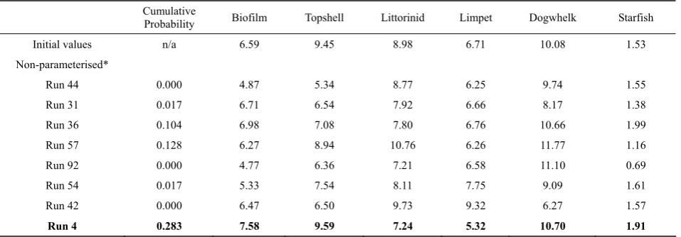
The clustering of the post disturbance rocky shore models is shown in Fig. 3, each scenario has eight clus-ters or post disturbance stable states with five or more predictions in it. Tables 9–11 show representative values for each of these clusters, for each of the different dis-turbance scenarios respectively. The closest agreement between the Bayesian network and the stable state is highlighted in bold.

2.4 Significant differences in microhabitats

Differences in microhabitats were found, with site 1 being significantly different from site 2, both in Sussex, and the site in County Durham being significantly dif

Fig. 3 Dendrograms showing similar clusters of commu-nities for (A) Scenario 1, (B) Scenario 2 and (C) Scenario 3

Table 9 Example results from Scenario 1

Cumulative

Probability Biofilm Topshell Littorinid Limpet Dogwhelk Starfish

Initial values n/a 5.07 9.45 8.98 6.71 10.08 3.05

Run 58 0.025 2.96 6.34 12.36 6.45 7.65 2.02

Run 55 0.025 3.20 5.56 9.06 7.02 6.33 2.10

Run 28 0.012 5.34 6.24 4.73 7.65 8.83 2.57

Run 85 0.030 4.97 9.58 9.68 7.83 7.01 2.36

Run 64 0.011 4.05 8.09 8.68 6.19 9.25 2.58

Run 68 0.026 5.13 6.60 9.65 6.42 9.00 2.63

Run 13 0.012 4.35 8.55 8.60 6.29 6.90 3.40

Run 99 0.031 5.15 9.59 9.49 9.91 8.29 2.57

A number of different stable states from clusters in Fig. 3a are identified – run 99 selected as best match to Bayesian network, based on highest cumulative probability.

Table 10 Example results from Scenario 2

Cumulative

Probability Biofilm Topshell Littorinid Limpet Dogwhelk Starfish

Initial values n/a 5.07 9.45 8.98 8.98 10.08 1.53

Run 17 0.034 5.50 6.80 12.70 7.38 11.10 1.78

Run 53 0.034 5.43 6.09 8.73 6.34 11.13 2.09

Run 57 0.031 3.70 6.38 9.00 9.81 8.98 1.64

Run 100 0.031 4.53 8.15 4.59 10.75 9.25 1.41

Run 72 0.049 4.45 8.81 10.72 7.55 10.17 1.40

Run 86 0.021 6.43 7.68 7.90 9.23 9.82 1.65

Run 77 0.026 4.44 6.22 7.62 7.89 5.93 1.34

Run 75 0.018 5.10 5.90 8.35 7.30 9.50 1.87

A number of different stable states from clusters in Fig. 3b are identified – run 72 selected as best match to Bayesian network.

Table 11 Example results from Scenario 3

Cumulative

Probability Biofilm Topshell Littorinid Limpet Dogwhelk Starfish

Initial values n/a 6.59 9.45 8.98 6.71 10.08 1.53

Non-parameterised*

Run 44 0.000 4.87 5.34 8.77 6.25 9.74 1.55

Run 31 0.017 6.71 6.54 7.92 6.66 8.17 1.38

Run 36 0.104 6.98 7.08 7.80 6.76 10.66 1.99

Run 57 0.128 6.27 8.94 10.76 6.26 11.77 1.16

Run 92 0.000 4.77 6.36 7.21 6.58 11.10 0.69

Run 54 0.017 5.33 7.54 8.11 7.75 9.09 1.61

Run 42 0.000 6.47 6.50 9.73 9.32 6.27 1.57

Run 4 0.283 7.58 9.59 7.24 5.32 10.70 1.91

A number of different stable states from clusters in Fig. 3c are identified – run 4 selected as best match to Bayesian network.

ferent from all sites is Sussex (Fig. 4). Differences are determined by overlap of the bootstrapped 95% Confi-dence radii, as indicated by the size of the bubble (see Stafford et al., 2012a for further details).

2.5 Review of transcriptome methods applied to rocky shore organisms

Fig. 4 Bootstrapped PCA, where each bubble represents a single site (bottom left to right = site 1, site 3, site 4, site 2, top = site 5)

Significant differences exist between site 1 and site 2, and between site 5 and all other sites, as defined by overlap of the bubbles.

strong laboratory-based tradition, largely because con-trolled conditions are required to understand the role of expressed genes (Kammenga et al., 2007; van Straalen and Roelofs, 2012). However, several rocky shore species have been subjects of transcriptome analysis, including microarrays specifically developed for mussels (Mytilus

spp. Gracey et al., 2008; Place et al., 2008) and the dog-whelk (Nucella lapillus Pascoal et al., 2013). Studies on

Littorina littorea have also been conducted, using human microarrays, which demonstrated > 18% cross reactivity (Larade and Storey, 2009). All of these species show sig-nificant changes in gene expression in relation to ‘stress’ in its broadest terms (Table 12). However, the studies carried out in field conditions, both on intertidal mussels, identified temporal changes associated with desiccation and temperature during the tidal cycle (Gracey et al., 2008), yet failed to identify spatial trends, such as latitu-dinal trends in gene expression (Place et al., 2008).

Table 12 Overview of transcriptome studies conducted on rocky shore invertebrates

Species Location Scientific name Analysis type Type of stress Overview of results Reference Dogwhelk North Wales, UK Nucella lapilus Custom

microarray

Endocrine disruptors Lab results of exposure to TBT tested against field results from different levels of TBT exposure.

Pascoal et al. (2013)

Mussel NW America (US

and Canada) Mytilus californianus Custom microarray Natural field conditions over large geographical area

Differences between site, but no latitudinal pattern. 12% of probes showed 2 fold changes between some sites.

Place et al. (2008)

Mussel California Mytilus californianus

Custom microarray

Natural field conditions over tidal cycle

Distinct gene expression profiles for moderate and severe heat stress at low water.

Gracey et al. (2008)

Periwinkle Canada (lab based study)

Littorina littorea Human microarray

Anoxia (lab based) >10 % of activated probes showed 2 fold changes in regulation.

Larade and Storey (2009)

While much work in gene expression focusses on understanding the roles of the genes up-or down- regu-lated, the fact that significantly different microhabitats, in terms of likely environmental stress can be identified (see previously), and gene expression changes with dif-ferent levels of stress, then quantifying overall changes in gene expression between ‘typical’ and ‘stressful’ habitats, or even the time from emersion taken to enter a heat or desiccation induced low tide stress phase, pre-sents a mechanism to identify changing stress levels on the shore, as a result of environmental change, and a possible mechanism to inform Bayesian networks about likely changes to community structure.

3 Discussion

This study has set out a framework for developing community models with incomplete knowledge of the

system under investigation, especially with regard to model parameters. It has also set out a framework for determining likely post-disturbance communities, as a result of factors including, but not limited, to climate change. Incorporation of predictive Bayesian networks allows the most likely possible ‘stable state’ models to be determined post disturbance, and the consideration of robustness of stable state models (i.e. the existence of similar communities examined through clustering algo-rithms) makes analysis of likely communities feasible, given the large number of stable states which can exist.

could therefore account for the wealth of molecular data that is increasingly available through approaches such analysis of the transcriptome of organisms. Under-standing how such transcriptomes may alter in response to significantly different microhabitats, and the impact of associated biological and physical stressors of these microhabitats is a first stage to reverse engineering the process to become predictive, and using transcriptome data to inform beliefs about the in situ stress acting on certain key species. These belief data can then be used to update probabilities in Bayesian networks, and allow us to consider likely community responses.

The current study provides a basic framework of techniques that can be used for predictive ecology, but it

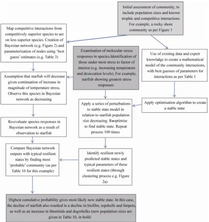
also highlights a number of areas that need considerable further development. A full process diagram of the framework, linked to a detailed example, is given in Fig. 5. However, as an example of how the process works, a detailed scenario is considered in Table 13.

The development of a simple, robust mathematical model of the real community is fundamental to the suc-cess of this approach. The model parameters are of less concern than the underlying mechanisms of the model (e.g. predation and competition), and clear focus needs to be placed on what is required from the prediction – for instance, are population sizes/density of the compo-nent species of the community required, or are the rela-tive strengths of organism interaction more important?

Fig. 5 Diagram of the key processes involved in predicting a new stable state, based on scenario 2 inTable 2 (reduction in starfish number)

Table 13 A simplified and illustrative example of how all component aspects of this paper can be incorporated into an assessment framework

Starfish Asterias rubens are examined from a range of microhabitats two weeks into a four week heat wave. Significant differences in microhabitat between an east and west facing breakwater occur after applying bootstrapped principle component techniques. Examination of the causing factors of these significant differences show only temperature and wave action differed between these microhabitats, however, wave action was similar on a breakwater facing north only 2 miles away, and this was not significantly different from either of the other two microhabitats.

Examination of gene expression for starfish in these microhabitats demonstrated that a suite of 36 genes showed increased levels of expression in the west facing microhabitat compared to the east facing. However 8 of these genes also showed differences in expression between the east and north facing habitat. During the heatwave, 50% mortality of starfish occurred on the west facing microhabitat, but no mortality on the north or east facing microhabitat.

We conclude, therefore, that the 28 (36-8) genes that showed increased expression in the west facing microhabitat are likely to be a good indication of significant heat stress in the starfish, and if the heat stress continues, may result in significant mortality of the starfish.

A different rocky shore is surveyed in a different year. Population density of different species is measured and from prior knowledge, trophic and competitive interactions are estimated, to form both a Bayesian network and a mathematical model of the relationships between organisms. The mathematical model is then combined with the optimisation algorithm to refine the interaction parameters and create a stable state.

Molecular surveys of starfish show very high levels of expression of the 28 genes identified above during the hottest weeks of the summer. Climate predictions indicate rising temperatures and prolonged heat waves in the next 20 years.

We can therefore predict that starfish are likely to undergo mortality if temperatures continue to rise, so we modify the Bayesian network to indicate they will decrease. We also optimise the mathematical model to find new stable states (given initial stochastic changes to population sizes of starfish).

We examine the stable states in the new mathematical model for resilience, and then compare the resilient states to the predictions of the Bayesian network.

The best fit of the two models is assumed to be the most likely new stable state that will occur on the shore. From the new parameters of the mathematical model, the new population sizes of each species can be determined.

A process diagram of this example is also given in Fig. 5. Note exam-ple is illustrative and the molecular data and community considered are speculative.

For example, in the present study, the focus of the pre-diction was on the population sizes of the component species. A combination of population size, activity of the species and a coefficient determined the levels of competition, predation or grazing between species. Such an approach is logical for rocky shore organisms, as some species are more active over the course of a tidal cycle than others (Little, 1989; Hutchinson and Wil-liams, 2003; Williams and Little, 2007; Stafford et al., 2012b,c). Equally, it is possible that activity levels could drop as a result of increasing stress, without effecting absolute number (especially if the prey supply in-creased). However, such an approach can be confusing

in terms of the parameters regarding competition and predation. The ‘control’ model, based on the initial parameterisation process showed a number of highly different activity levels to what was initially proposed, and in particular, showed a big, and unrealistic discrep-ancy in the activity levels of the three grazing molluscs. However, examination of competition and predation coefficients indicated these activity levels were ac-counted for in the values of the other model coefficients. This is exemplified by the fact that topshells showed far greater activity then limpets in the parameterised rocky shore model, but the topshell -> limpet completion co-efficient was far lower than the initial value given. Re-moval of parameters such as ‘activity’ may be important if comparisons between species interactions need to be considered as part of the prediction of the model; how-ever, this may effect population estimates, and care to select the best mathematical model through comparison with Bayesian networks are needed. An alternative ap-proach may be to refine the criterion of stability. While stable states are essential for this technique, due to the location of local minima in the search landscape, stabil-ity may be defined as something other than change in each species’ population level. Although this approach is intuitive, activity levels and populations sizes can interact, as described above, and stability on criteria such as energy flow (per species) may provide a less ambiguous response, although considerably harder to parameterise though best guess approaches. While mathematically complex concepts of stability exist (e.g. time series measures such as those described in Ives et al. 2003), the behaviour of these during regime shift is rather chaotic (Biggs et al., 2009; Stafford et al., 2011). These measures also reduce the degree of intuition into the results, which a direct measure of community, such as population size across all species, provides. However, this does not mean that alternative measures of stability should not be considered in future studies.

largely this is in terms of ranking species in terms of competitive superiority, rather than exact knowledge of determination of exact model parameters.

Given the framework provided here, the predictive modelling approach next needs to be applied to a range of real ecological systems, which have been extensively studied both pre- and post-regime shift. Of particular interest may be intertidal and shallow marine communi-ties in areas where there are large seasonal changes in community structure (e.g. rocky shore communities in southern China which undergo tropical summers, but temperate winters: Williams, 1993), as these may be better understood. Further experimental measurements can then be taken, as opposed to relying on existing data from historical datasets where regime shift is known to have occurred.

In addition, transcriptome data, such as from RNA microarrays, needs to be collected from organisms in their natural environments, as well as in controlled laboratory conditions (as per Pascoal et al., 2013). Ide-ally, stress response genes need to be linked to reduction in fitness or near mortality of species, since it is impor-tant to determine acute stress from normal biochemical and physiological adaptation to environmental condi-tions. For example, Littorina littorea shows consider-able response to anoxia in terms of gene expression on human microarrays (Larade and Storey, 2009), and al-though anoxia is common in this species, excessive lev-els of it will decrease fitness, by limiting its energy budget through respiration. Hence early expression of these genes within a tidal cycle will likely mean greater levels of anoxia stress are occurring, and prolonged ex-pression is likely to result in decreased fitness. In this anoxia response, many of these genes that have been up- or down-regulated may be general stress response genes, and analysis of how these genes change occur in re-sponse to different microhabitats may provide informa-tion on likely stressors to an integrated suite of envi-ronmental effects, which will occur in natural habitats. Similarly, given the multitude of possible stressors in natural environments, it is not wholly surprising that trends in gene expression may not follow latitudinal gradients, and emphasis needs to be placed on deter-mining different microhabitats in terms of physical and biological factors. In essence, determining significant differences in microhabitats is akin to a ‘natural’ ex-perimental manipulation, and analysis of principle components may indicate the key factors that differ be-tween different microhabitats. Hence, as indicated in an idealised example in Table 13, it may be possible to

determine significant differences between habitats in terms of single stressors, such as temperature, and in-vestigate the genes which are differentially over or un-der expressed in this habitat, whereas inflicting stress in laboratory conditions will stimulate a range of stress response genes. Further focus on the relative importance of different microhabitat factors may need to be consid-ered, however. For example, temperature or desiccation rates may be key physical drivers of stress, yet inter-specific competition between very ecologically similar species, such as Littorina saxatilis and Melarharphe neritoides may be unimportant when there is strong in-traspecific competition. Comparing molecular stress responses to real microhabitats and measureable eco-logical features of the environment may not only pro-vide information to inform predictive models of suscep-tible species, but may also indicate the most important drivers of regime shift in a variety of communities.

This study has focussed greatly on climate induced regime shift, but in fact, the modelling techniques here can be used to assess any form of disturbance, and de-termine not only if new stable states are formed, but what these stable states may be. For example, invasive species (either climate driven or otherwise) can cause large changes in community structure (Pyšek et al., 2012), harvesting of resources (such as through fisheries) can also affect community structure (Magnússon, 2005). The inclusion of molecular data is also not limited to climate effects, but more limited to factors that create internal physiological stress. However, as demonstrated by the uses of microarrays in rocky shore ecology, pre-dictions of the effect of factors such as pollution, anoxia (caused through eutrophication as a result of changes in land use or urbanisation) can all be assessed using these integrated methods.

References

Biggs R, Carpenter SR, Brock WA, 2009. Turning back from the brink: Detecting an impending regime shift in time to avert it. Proc. Nat. Acad. Sci. 106: 826–831

Cozman F, 2001. JavaBayes-version 0.346. Available at: http:// www. cs.cmu.edu/~javabayes/Home/

Dudgeon SR, Aronson RB, Bruno JF, Precht WF, 2010. Phase shifts and stable states on coral reefs. Ma.r Ecol. Prog. Ser. 413: 201–216.

Gilman SE, Urban MC, Tewksbury J, Gilchrist GW, Holt RD, 2010. A framework for community interactions under climate change. Trends Ecol. Evol. 25: 325–331.

elasmo-branchs based on dietary data and Bayesian networks. Ecol. Indicators 1: 197–211.

Harrold C, Reed DC, 1985. Food availability, sea urchin grazing, and kelp forest community structure. Ecology 66: 1160–1169. Holland JH, 1992. Adaptation in Natural and Artificial Systems.

Cambridge MA: MIT Press.

Hosack GR, Hayes KR, Dambacher JM, 2008. Assessing uncer-tainty in the structure of ecological models through a qualita-tive analysis of system feedback and Bayesian belief networks. Ecol. Applications 18: 1070–1082.

Hutchinson N, Williams GA, 2003. An assessment of variation in molluscan grazing pressure on Hong Kong rocky shores. Mar. Biol. 142: 495–507.

IPCC, 2007. Climate Change 2007: Synthesis Report. Geneva: IPCC. Ives AR, Dennis B, Cottingham KL, Carpenter SR, 2003.

Esti-mating community stability and ecological interactions from time-series data. Ecol. Monog. 73: 301–330

Kammenga JE, Herman MA, Ouborg NJ, Johnson L, Breitling R, 2007. Microarray challenges in ecology. Trends Ecol. Evol. 22: 273–279.

Knowlton N, 1992. Thresholds and multiple stable states in coral reef community dynamics. Am. Zool. 32: 674–682.

Konar B, Estes JA, 2003. The stability of boundary regions be-tween kelp beds and deforested areas. Ecology 84: 174–18. Larade K, Storey KB, 2009. Living without oxygen: anoxia-

re-sponsive gene expression and regulation. Cur. Genom. 10: 76–85. Lewontin RC, 1969. The meaning of stability. Brookhaven Symp.

Biol. 22: 13–24.

Little C, 1989. Factors governing patterns of foraging activity in littoral marine herbivorous molluscs. J. Molluscan Stud. 55: 273–284.

Little C, Williams GA, Trowbridge CD, 2009. The Biology of Rocky Shores. Oxford: Oxford University Press.

Magnússon KG, 1995. An overview of the multispecies VPA: Theory and applications. Rev. Fish Biol. Fish. 5: 195–212 May RM, 1977. Thresholds and breakpoints in ecosystems with a

multiciplicity of stable states. Nature 269: 471–477.

Menge BA, 1972. Foraging strategy of a starfish in relation to actual prey availability and environmental predictability. Ecol. Monog. 42: 25–50.

Mumby PJ, 2007. Thresholds and the resilience of Caribbean coral reefs. Nature 450: 98–101.

Nakamura Y, Oke TR, 1967. Wind, temperature and stability con-ditions in an east-west oriented urban canyon. Atmospheric Environ. 22: 2691–2700.

Pascoal S, Carvalho GR, Vasieva O, Hughes RN, Cossins A et al., 2013. Transcriptomics and in vivo tests reveal novel mechanisms underlying endocrine disruption in an ecological sentinel Nucella lapillus. Mol. Ecol. DOI: 10.1111/mec.12137 Pearson RG, Dawson TP, 2003. Predicting the impacts of climate

change on the distribution of species: Are bioclimate envelope models useful? Global Ecol. Biogeog. 12: 361–371.

Peters RL, Lovejoy TE, 1994. Global Warming and Biological Diversity. New Haven, CT: Yale University Press.

Peterson CH, Lubchenco J, 1997. Marine Ecosystem Services. In: Daily CG ed. Nature’s Services. Washington DC: Island Press 177–194. Petraitis PS, Dudgeon SR, 1999. Experimental evidence for the

origin of alternative communities on rocky intertidal shores.

Oikos 84: 239–245.

Petraitis PS, Dudgeon SR, 2004. Do alternative stable states exist in the Gulf of Maine rocky intertidal zone? A comment. Ecol-ogy 85: 1160–1165.

Place SP, O’Donnell MJ, Hofmann GE, 2008. Gene expression in the intertidal mussel Mytilus californianus: Physiological re-sponse to environmental factors on a biogeographic scale. Mar. Ecol. Prog. Series 356: 1–14.

Pyšek P, Jarošík V, Hulme PE, Pergl J, Hejda M et al., 2012. A global assessment of invasive plant impacts on resident species, communities and ecosystems: The interaction of impact meas-ures, invading species' traits and environment. Glob. Change Biol. 18: 1725–1737.

R Development Core Team 2012. R: A Language and Environ-ment for Statistical Computing. Vienna: R Foundation for Sta-tistical Computing.

Somero GN, 2002. Thermal physiology and vertical zonation of intertidal animals: Optima, limits, and costs of living. Integ. Comp. Biol. 42: 780–789.

Stafford R, 2002. The role of environmental stress and physical and biological interactions on the ecology of high shore Lit-torinids. In: A Temperate and A Tropical Region. Ph.D. thesis, University of Sunderland, UK.

Stafford R, Davies MS, Williams GA, 2008. Parameterization and prediction of community interaction models using stable-state assumptions and computational techniques: An example from the high rocky intertidal. Biol. Bull. 215: 155–163.

Stafford R, Goodenough AE, Slater K, Carpenter W, Collins L et al., 2012a. Inferential and visual analysis of ethogram data us-ing multivariate techniques. Anim. Behav. 83: 563–569. Stafford R, Davies MS, Williams GA, 2012b. Cheats in a

coop-erative behaviour? Behavioural differences and breakdown of cooperative behaviour in aggregating, intertidal littorinids (Mol-lusca). Mar. Ecol. 33: 66–74.

Stafford R, Davies MS, Williams GA, 2012c. Misinterpreting the potential benefits of aggregation for reducing desiccation in the intertidal: A simple analogy. Mar. Ecol. 33: 512–515 Stafford R, Williams RL, Kirkhope CL, 2011. Complex systems :

What ecology teaches us about the credit crisis and long-term economic recovery. Prog. Econ. Res. 20: 307–317.

Sutherland JP, 1974. Multiple stable points in natural communities. Am. Nat. 108: 859–873.

van Straalen NM, Roelofs D, 2012. An Introduction to Ecological Genomics. 2nd _{edn. Oxford: Oxford University Press.}

Walker B, Salt D, 2006. Resilience Thinking: Sustaining Ecosystems and People in a Changing World. Washington DC: Island Press Williams GA, 1993. Seasonal variation in algal species richness

and abundance in the presence of molluscan herbivores on a tropical rocky shore. J. Exp. Mar. Biol. Ecol. 167: 261–275. Williams GA, Little C, 2007. Foraging Behaviour. In: Denny M,

Gaines S ed. The Encyclopedia of the Rocky Intertidal. Berke-ley: California University Press, 239–242.

Williams GA, Morritt D, 1995. Habitat partitioning and thermal tolerance in a tropical limpet Cellana grata. Mar. Ecol. Prog. Ser. 124: 89–103.