Unresolved fine scale structure in solar coronal loop tops

C

2014. The American Astronomical Society. All rights reserved. Printed in the U.S.A.

UNRESOLVED FINE-SCALE STRUCTURE IN SOLAR CORONAL LOOP-TOPS

E. Scullion1,2, L. Rouppe van der Voort1, S. Wedemeyer1, and P. Antolin3 1_{Institute of Theoretical Astrophysics, University of Oslo, P.O. Box 1029, Blindern, NO-0315 Oslo, Norway}

2_{Trinity College Dublin, College Green, Dublin 2, Ireland;[email protected]} 3_{National Astronomical Observatory of Japan, 2-21-1 Osawa, Mitaka, Tokyo 181-8588, Japan}

Received 2014 August 7; accepted 2014 October 1; published 2014 November 24

ABSTRACT

New and advanced space-based observing facilities continue to lower the resolution limit and detect solar coronal loops in greater detail. We continue to discover even finer substructures within coronal loop cross-sections, in order to understand the nature of the solar corona. Here, we push this lower limit further to search for the finest coronal loop substructures, through taking advantage of the resolving power of the Swedish 1 m Solar Telescope/CRisp Imaging Spectro-Polarimeter (CRISP), together with co-observations from theSolar Dynamics Observatory/Atmospheric Image Assembly (AIA). High-resolution imaging of the chromospheric Hα656.28 nm spectral line core and wings can, under certain circumstances, allow one to deduce the topology of the local magnetic environment of the solar atmosphere where its observed. Here, we study post-flare coronal loops, which become filled with evaporated chromosphere that rapidly condenses into chromospheric clumps of plasma (detectable in Hα) known as a coronal rain, to investigate their fine-scale structure. We identify, through analysis of three data sets, large-scale catastrophic cooling in coronal loop-tops and the existence of multi-thermal, multi-stranded substructures. Many cool strands even extend fully intact from loop-top to footpoint. We discover that coronal loop fine-scale strands can appear bunched with as many as eight parallel strands within an AIA coronal loop cross-section. The strand number density versus cross-sectional width distribution, as detected by CRISP within AIA-defined coronal loops, most likely peaks at well below 100 km, and currently, 69% of the substructure strands are statistically unresolved in AIA coronal loops.

Key words: methods: data analysis – methods: observational – techniques: image processing – techniques: spectroscopic – telescopes

Online-only material:color figures

1. INTRODUCTION

It has long been claimed (for, e.g., Gomez et al.1993, and earlier) that coronal loops consist of bundles of thin strands, to scales below the current instrumental resolution. Today, that statement continues to remain as prevalent as ever. Coronal loops were first detected in coronagraphic observations in the 1940s (Bray et al. 1991). These loops are observed to extend into the low plasma-βenvironment of the solar corona, arching over active regions, and are filled with relatively dense plasma (in the range of ∼108_–1010 _cm−3_{) and confined by}

a dipole-like magnetic field (Aschwanden2004; Reale 2010, and references therein). Coronal loops are observed to have a broad range of temperatures, and they are observed in extreme ultraviolet (EUV) from ∼105_{K (cool loops) to a few 10}6_K

(warm loops) and up to a few 107K (flaring loops). In coronal loops, neighboring magnetic field lines are considered to be thermally isolated; hence, each field line can be considered independently, which we call a “strand” herein.

To explain the nature of coronal loops is to understand the origin of solar coronal heating. One fundamental issue is that we do not know what the spatial scale of the mechanisms that heat the solar corona is (Reale2010). It has been considered that in order to form stable overdense, warm coronal loops, it may be required to assume that coronal loops consist of unresolved magnetic strands, each heated impulsively, non-uniformly, and sequentially (Gomez et al.1993; Cargill1994; Klimchuk2000; Klimchuk & Cargill2001; Reale et al.2005; Klimchuk 2006; Klimchuk et al. 2008). At a typical spatial resolution (of most current space-based instruments observing

from EUV to higher energies) of ∼1000 km (∼1.5: 1 arcsec () ≈720 km), it is likely that most observations represent superpositions of hundreds of unresolved strands that can exist at various stages of heating and cooling (Klimchuk

2006). Other studies based both on models and on analysis of observations independently suggest that elementary loop components should be even finer, with typical cross-sections of the strands on the order of 10–100 km (Beveridge et al.2003; Cargill & Klimchuk 2004; DeForest 2007). The space-based (Hinode; Kosugi et al.2007) EUV Imaging Spectrometer (EIS; Culhane et al. 2007) has been used together with the Solar Dynamics Observatory(SDO)/Atmospheric Image Assembly (AIA; Lemen et al.2012) to investigate the fundamental spatial scales of coronal loops; the results suggest that most coronal loops remain unresolved (Ugarte-Urra et al. 2012) given the 1.2 (∼860 km) and 2(∼1440 km) resolution ofSDO/AIA and Hinode/EIS, respectively.

However, contrary to this, Brooks et al. (2012) presented results of multi-stranded loop models calculated at a high reso-lution. They show that only five strands with a maximum radius of 280 km are required in order to reproduce the observed coro-nal loops, and a maximum of only eight strands where needed to reproduce all of the detected loops. More recently (2012 July 11), the High-resolution Coronal Imager (Hi-C; Cirtain et al.

The Astrophysical Journal, 797:36 (10pp), 2014 December 10 Scullion et al. In other words, the finest-scale substructures of coronal loops

are already observable. Other studies concerning the variations of intensity across a variety of hot loops, co-observed by AIA and Hi-C, have continued to speculate on whether or not strand substructures could potentially exist well below what Hi-C or AIA can resolve (Peter et al.2013). Most recently, Winebarger et al. (2014) performed a statistical analysis on how the pixel intensity scales from AIA resolution to Hi-C resolution. They claim that 70% of the Hi-C pixels show no evidence for sub-structuring, except in the moss regions within the field of view (FOV) and in regions of sheared magnetic field.

There is strong evidence to suggest that coronal loops are, in-deed, so finely structured when we consider loop legs from coor-dinated observations involving high-resolution spectral imaging with ground-based instruments. Antolin & Rouppe van der Voort (2012) performed a detailed and systematic study of coronal rain (Kawaguchi1970; Schrijver2001; De Groof et al.2004) via the Swedish 1 m Solar Telescope (SST; Scharmer et al. 2003a)/ (CRISP; Scharmer et al.2008) instrument at very high spatial and spectral resolutions (0.0597 image scale). They detected narrow clumps of coronal rain in Hα down to the diffraction limit (130 km) in the cross-sectional area, with average lengths between∼310 km and ∼710 km and widths approaching the diffraction limit of the instrument. These measurements where repeated for on-disk coronal rain by (Antolin et al.2012). Coro-nal rain is considered to be a consequence of a loop-top thermal instability driving catastrophic cooling of dense plasma (see Antolin et al. 2010; Antolin & Rouppe van der Voort 2012, and references therein). Radiation cooling of dense evaporated plasma (filling coronal loops) leads to the onset of plasma de-pletion from the loops, slowly at first and then progressively faster.

From an observational standpoint, the next step is to reveal evidence for substructuring along the full length of the coronal loop, from loop-top toward footpoint, and directly measure the threaded nature of coronal loop-tops using CRISP (with the most powerful resolving capability), in order to adequately test the existence of unresolved structure in the outer solar atmosphere. Observations from the ground-based instruments, such as CRISP, have obvious advantages over space-based facilities, with respect to resolving power given their much larger apertures. Analysis of the Hαline core from such imaging spectropolarimeters provides an excellent tracer of the magnetic environment of the lower solar atmosphere (Leenaarts et al.

2012). Through coordinated observations of coronal loops, with AIA and CRISP, we can use imaging in Hαas a proxy for revealing the internal magnetic structure of coronal loops. As discussed in Antolin & Rouppe van der Voort (2012), it is possible that there is a strong dynamic coupling between neutrals and ions in coronal loops during the formation of coronal rain. As a result, the rain can become observable in the Hα to reveal, in great detail, the topological structure of the local coronal magnetic field. The condensation process initially generates small rain clumps in situ within coronal loop-tops until the point where the mass density of the rain becomes large enough, leading to a flow of clumps toward the loop footpoints (Fang et al. 2013). The lower limit (in spatial scales), with respect to the size distribution of these clumps, is dependent upon the magnetic fine-scale structuring of coronal loops. Momentarily and as a consequence of the thermal properties of the dense plasma undergoing rapid condensation, the Hα signal is detectable within post-flare coronal loops because the atmospheric conditions in the loops match that of

the chromosphere. Fundamentally, the magnetic substructuring of the coronal loops near loop-tops should remain the same or similar for all coronal loops (flaring and non-flaring). However, the possibility of probing the fine-scale magnetic structure of coronal loops during the post-flare phase with Hα via high-resolution imaging can present itself.

In this paper, we report on the distribution of threaded substructures within a coronal loop from loop-top toward footpoint via direct imaging of coronal loop cross-sections through a coordinated SST andSDOanalysis, which comprises three data sets.

2. OBSERVATIONS

CRISP, installed at the SST, is an imaging spectropolarimeter that includes a dual Fabry–P´erot interferometer, as described by Scharmer (2006). The resulting FOV is about 55×55. CRISP allows for fast wavelength tuning (∼50 ms) within a spectral range and is ideally suited for spectroscopic imaging of the chromosphere. For Hα656.3 nm, the transmission FWHM of CRISP is 6.6 pm and the prefilter is 0.49 nm. The image quality of the time series data is greatly benefited from the correction of atmospheric distortions by the SST adaptive optics system (Scharmer et al.2003b) in combination with the image restora-tion technique Multi-Object Multi-Frame Blind Deconvolurestora-tion (MOMFBD; van Noort et al.2005). Although the observations suffered from seeing effects, every image is close to the theo-retical diffraction limit for the SST. We refer to van Noort & Rouppe van der Voort (2008) and Sekse et al. (2013) for more details on the MOMFBD processing strategies applied to the CRISP data. We followed the standard procedures in the reduc-tion pipeline for CRISP data (de la Cruz Rodr´ıguez et al.2014), which includes the post-MOMFBD correction for differential stretching suggested by Henriques (2012).

We explore the fully processed data sets with Vissers & Rouppe van der Voort (CRISPEX 2012), a versatile code for analysis of multi-dimensional data cubes. We have compiled, with these reduction methods, three data sets from excellent periods of seeing that contain active region coronal loops within the CRISP FOV.

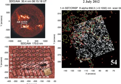
Data set A. A mosaic observing sequence (presented in Figures1and2) was set to repeat once, with a line scan in Hα at four wavelength positions (as presented in Figure2), for the 280×180FOV containing active region (AR) 11515 on 2012 July 2, centered at [−225,−275] in solarx/y. The pointing per position was preset to 5.5 s, including 1.5–2 s for the telescope to change pointing. The total duration of the observation was 600 s, so there were 108 pointing sequences in this interval with a repeat of 54 positions resulting in a cadence of 300 s between 08:10 and 08:20 UT. The co-alignment between CRISP and AIA for the mosaic observation is presented in Figure1.

Data set B. A time series with six wavelength-point spectral scans in Hαwith an effective cadence of 19 s (after frame selec-tion on the MOMFBD restored data) pointed at [−349,−329] in solarx/yon 2012 July 1, centering on AR 11515 between 15:08 and 16:31 UT.

Data set C. A time series with 43 wavelength-point spectral scans in Hα with an effective cadence of 10.8 s pointed at [−818,179] in solar x/y on 2011 September 24, centering on AR 11302 between 10:17 and 11:02 UT.

Figure 1.Overview of the CRISP 54 grid mosaic of July 2 AR 11515 is presented in the context ofSDO/AIA 170.0 nm (lower left) and 30.4 nm (upper left, with the extended FOV boxed) passbands. The order of the 5 minute scan sequence (which was repeated once over a 10 minute interval) is depicted (lower left) as a series of overlapping segments corrected for solar tilt. The accurate co-alignment of bright points in 170.0 nm (contoured in green and yellow), with coincident bright points in the grayscale Hαcontinuum image from CRISP, is presented for grid segment No. 54 (right).

(A color version of this figure is available in the online journal.)

bright points exist as discrete, bright, and relatively long-lived features that exist in both quiet-Sun, active regions, and, to a lesser extent, coronal holes. They are well distributed over the solar disk and can be clearly identified in the upper photospheric AIA 170.0 nm channel (log T=3.7). Our spectral line scan of Hαincludes nearby continuum positions in both the blue wing (−0.1032 nm) and red wing (+0.1032 nm) for all our data sets. In the case of data set A, each grid in the mosaic sequence at the near-continuum spectral position was independently aligned to the corresponding SDO/AIA 170.0 nm (derotated FOV to compensate for solar rotation) in space and time. This accurate method for achieving a sub-AIA pixel accuracy in the co-alignment between the space-based SDO/AIA and ground-based SST/CRISP images is displayed in Figure1(right). The same method was also applied in regard to the co-alignment of data sets B and C.

3. RESULTS

Data set A, composed of the mosaic coronal loop observation, contains primarily warm active region loops. We examine the coronal loop multi-thermal substructures of active region loops in the following section. After that, we will focus on the substructures within loops in data sets B and C, which both contain hot, post-flare coronal loops. In that section, we will investigate the substructure of hot post-flare coronal loops that have experienced strong chromospheric evaporation.

3.1. Active Region Loops

In Figure2, we present the reduced and reconstructed mosaic images for the Hαline scan of AR 11502 from the 2012 July 2.

The line scan positions include−0.1032 nm (a) and−0.0774 nm (c) in the blue wing, relative to the line core (b) and one position in the red at +0.1032 nm (d). The green box in Figure 2(a) indicates the location of a high speed chromospheric upflow with a strong Doppler shift with an equivalent velocity of∼47 km s−1_.

Interestingly, the trajectory of this high-speed upflow, in the Hα green box, coincides with the footpoint of a large-scale loop in apparent downflow in the Hαyellow box. The imposing loop-like structure, which extends above the sunspot group, is clearly observed in the red wing of Hα, as revealed in the yellow box in Figure2(d). This structure is co-spatial with EUV coronal loops, as observed inSDO/AIA, and its loop-top fine-scale structure is the focus of our investigation.

The Astrophysical Journal, 797:36 (10pp), 2014 December 10 Scullion et al.

(a) (b)

(c) (d)

Figure 2.CRISP Hαline scan images for the reconstructed 54 grid mosaic of July 2, for the time interval 08:15:05–08:20:00 UT. The line scan includes two far wing positions: (a) in the far blue-wing and (d) in the far red-wing. Panel (c) samples the fast spicular structures in the near blue-wing of Hα, and panel (b) samples the upper chromospheric plasma in the Hαcore, revealing a complex network of chromospheric loops and dynamic fibrils. The line scan positions, relative to the solar atlas Hαprofile, are presented in the subfigure of panel (a), and the specific wavelengths of the scan are detailed in the panel titles. The green and yellow boxes mark features of interest for our investigation.

(A color version of this figure is available in the online journal.)

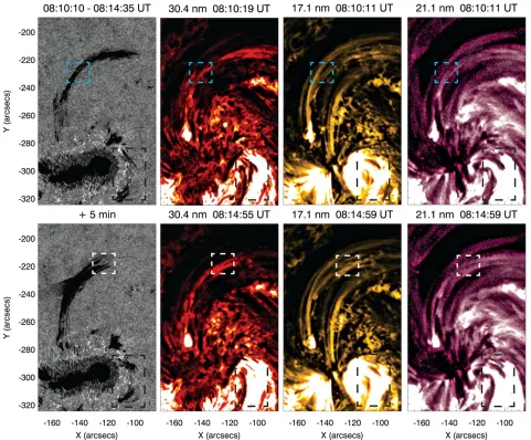
dense plasma near the loop-top. The blue dashed boxes in the top row correspond to the FOV of the loop-leg which will be examined in more detail.

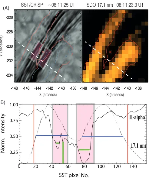
In Figures 4 and 5, panel (A), we present the zoomed-in regions from Figure3, blue dashed box (loop-leg) and white dashed box (loop-top), respectively. Here, we reveal in great detail that both the loop-tops and loop-legs consist of bundles of fine-scale strand substructures, which can remain connected along the length of the loop. The fine strands, identifiable within the pink boxed regions in Figure4, panel (A), and white dashed in Figure5, panel (A), appear to be parallel with each other and exist contained within the AIA-defined loop boundary (see the blue dashed line in Figure5, panel (A)). In Figure4, panel (B), the data cross-cuts (extracted from the diagonal dashed slit of Figure 4, panel (A)) demonstrate the substructured nature of the loop in Hαwithin, and are not necessarily confined to, the double-peak profile representing 17.1 nm normalized intensity. The 17.1 nm loop system boundary (marked by the vertical red lines in Figure4, panel (B)) has a maximum cross-sectional width of 3–4 Mm and also appears structured down to the resolution limit of the AIA instrument. The AIA temperature response function for the 17.1 nm passband has its maximum around 0.9 MK. We find that the FWHM of each of the AIA

Figure 3.Large-scale, high-velocity downflow in the Hαfar wing image (+0.1032 nm) is presented in the first panel of the top row, and its evolution after five minutes is presented in the first panel of the bottom row. The co-spatial and co-temporal warm coronal loop is visible in theSDO/AIA Heii30.4 nm (second column), Feix

17.1 nm (third column), and Fexiv21.1 nm (fourth column) images as shown. The blue dashed box (top row) represents the FOV of Figure4, for a closer inspection of the coronal loop-leg substructures. The white dashed box in the bottom row represents the coronal loop-top and the FOV of Figure5. The black dashed box reveals an adjacent closed hot-loop system, with co-spatial dark flows (in Hα) that extend along the loop-legs toward the footpoints.

(A color version of this figure is available in the online journal.)

and are bounded by, the curved blue dashed lines of the AIA 17.1 nm loop boundary. This is the same loop system connecting the loop-leg from Figure4. The finest detectable strands exist within Region 3, and they all extend uniformly in length across the FOV for at least 1100 km. The right-most strand channel from Region 2 has a cross-sectional width similar to that of the broadest strand from the loop-leg section. However, the most commonly occurring strand cross-section, from both loop-top and loop-leg sections, is 130 km.

We have found multi-stranded and multi-thermal fine-scale structuring within warm active region coronal loops in both loop-top and loop-leg sections. However, is this scenario con-sistent with hotter post-flare loops, which can undergo a more widespread and intense footpoint heating?

3.2. Post-flare Loops

Figures6and7display the overlays of the hot post-flare loop system of data set B, which consists of CRISP observations centered on AR 11515 (same active region as data set A,

The Astrophysical Journal, 797:36 (10pp), 2014 December 10 Scullion et al.

17.1 nm H-alpha

0.25 0.50 0.75 1.00

0 20 40 60 80 100 120 140

Norm.

Int

ensit

y

SST pixel No.

(A)

(B)

Figure 4. Fine-scale, multi-stranded, and multi-thermal substructures are detected within the coronal loop-leg and are presented here for the white dashed box region of Figure3. The Hαline position of +0.1032 nm image (grayscale) is shown in panel (A) together with the near-simultaneous and co-spatial AIA 17.1 nm image. The coronal loop in 17.1 nm is contoured (solid red line) and overlaid in both images to compare with the Hαmulti-threaded component of the loop. A white dashed diagonal slit and two pink boxed regions are extracted, and their normalized intensity profiles are plotted in panel (B) for comparison of both spectral lines. The data cross-cuts for Hα(solid curve) are overlaid with 17.1 nm (dotted curve). The blue solid lines presented the FWHM of the double-peaked 17.1 nm profile, and the green lines demarcate the locations of fine-scale strands that exist within the loop system.

(A color version of this figure is available in the online journal.)

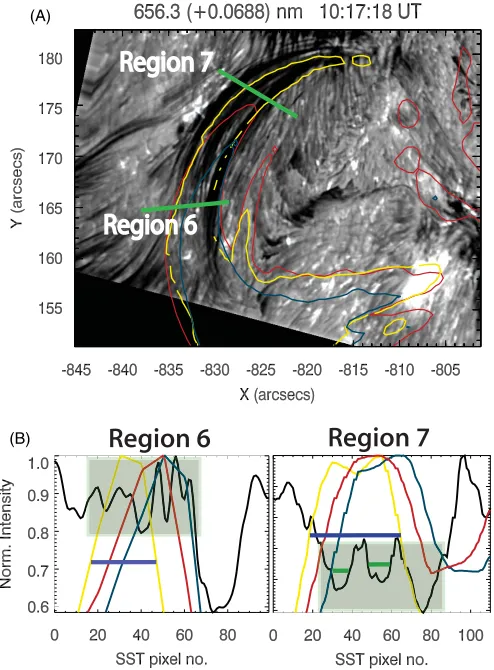
Figures6and7, panel (B), display similar fine-scale structuring very much confined within the post-flare loops. Again, we detect double-peak structures in many of the AIA channels (notably in the 21.1 nm red curves) and multiple strands in the Hαline position, indicating the presence of narrower threads well below the instrumental resolution of AIA. The green boxed regions in Figures6and7, panel (B), highlight the sections of the cross-cuts where we have an overlap between AIA loops and structure in Hα, which again implies a coincidence in the location of the formation of the lines to within the coronal loop itself. The cross-sectional width measurements of all the fine-scale strands, within the full length of the loop system from loop-top to footpoint, will be accumulated together with data set A for statistical comparison of the variation in the range of scales present within the loop systems.

Data set C consists of CRISP observations centered on a region that hosted a GOES X1.9 class flare (post-impulsive phase close to the northeast solar limb) on 2011 September 24. In Figures8and9, panel (A), we present images of the Hαred-wing (Figure8) and blue-wing (Figure9) grayscaled images, which are almost coincident in observation time at 10:17 UT (within the same line scan with one line scan taking 4.2 s). These images are again overlaid with contours from AIA 17.1 nm (yellow), 21.1 nm (red), and also 19.3 nm (dark blue), for the post-flare

Region 1 Region 1

5500

5000

4500

4000

3500

0 5 10 15 20 0 5 10 15 0 5 10 15

CRISP Int

ensit

y Scale

SST pixel No.

Region 2 Region 2

Region 3 Region 3 Region 1

Region 1

Region 2 Region 2

Region 3 Region 3 (A)

(B)

Figure 5.Fine-scale, multi-stranded and multi-thermal substructures are de-tected within the coronal loop-top and are presented here for the blue dashed box region of Figure3. The Hαline position of +0.1032 nm image (grayscale), is shown in panel (A), together with the near-simultaneous and co-spatial AIA 17.1 nm image. Regions 1–3 in panel (A) are selected for investigation of the Hαintensity profile as data cross-cuts along the loop-top system, which are represented in panel (B). As with Figure4, parallel strands are identified using green lines separated by pink lines marking strand channels. Regions 2 and 3 are particularly highly structured in the Hαline profiles.

(A color version of this figure is available in the online journal.)

loop system 56 minutes after the flare GOES X-ray peak. During this phase, we again expect to see evidence of coronal rain formation, with a characteristic signature in Hα. In data set C, catastrophic cooling is indeed present across the entire post-flare loop and the opposing flows as the rapidly cooled coronal rain depletes from the loop-top under the action of gravity is exquisitely revealed. We can clearly detect opposing, dark Doppler flows running along both legs of the loop system, as absorption in Hα(as defined by AIA contours), in the red-wing for the left-side leg (Figure8) and in the blue-wing for the right-side leg (Figure9). The Doppler signature in the loop reveals the geometrical nature of the loop itself. In the line core images, we can detect the structure of the loop-top where there is a net zero Doppler shift, which is in agreement with the location of the observed loop-top in the EUV channels and confirmation that the hot and cold plasma must be co-located within the same loop structure.

Region 4

Region 4

Region 4

(A)

(B)

Figure 6.Co-temporal and co-spatial Hαnear red-wing images (grayscale), together with overlaid contours (17.1 nm: yellow and 21.1 nm: red), are presented in panel (A). The observations consist of a snapshot of a post C8.2 class flare system from 2012 July 1 (data set B). Panel (B) presents the normalized intensity cross-cuts of the post-flare loop-top (solid green line Region 4 in panel (A)) for the associated Hαsignal (black curve) along with the respective curves of the 17.1 nm (yellow) and 21.1 nm (red) channels, as is contoured in panel (A). The shaded green boxes represent examples of associated fine-scale structures in Hαand the EUV lines from which we extract measurable strand cross-sections for our statistical sample. The blue horizontal lines represent the well-defined and measurable cross-sections of the EUV loops in contrast with the fine-scale structuring in Hα.

(A color version of this figure is available in the online journal.)

normalized intensity cross-cuts from both Hα(black curve) and the EUV channels (17.1 nm: yellow and 21.1 nm: red curves) for slit Regions 6–8. Again, we can reveal fine-scale structuring within the Hαintensity profiles (from within the green shaded boxes) in both Figures8and9that are co-spatial with singly peaked profiles in the EUV channels. In both Regions 7 and 8, we can detect similarly scaled strands and a variable range in the cross-section strand number density of, typically, three to five clearly defined parallel strands. The data cross-cuts from each of the AIA passbands contoured here are also overlaid. The EUV loop intensity profiles appear to have cross-sectional widths in the range of 25–40 SST pixels (approximately five to six times greater than fine-scale Hαstrands within them as marked by solid green lines), as marked with the solid blue lines in panel (B) of both Figures8and9. These measurements are comparable with those profiles deduced from data set B, which was a substantially weaker post-flare loop system, and

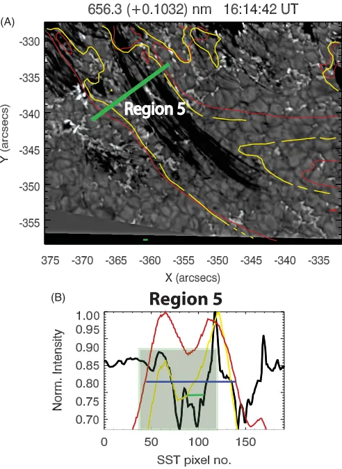
Region 5

Region 5

(A)

(B)

Figure 7.Co-temporal and co-spatial Hα far red-wing images (grayscale), together with overlaid contours (17.1 nm: yellow and 21.1 nm: red), are presented in panel (A). The observations consist of a snapshot of a post C8.2 class flare system from 2012 July 1 (data set B). Panel (B) presents the normalized intensity cross-cuts of the post-flare loop-leg (solid green line Region 5 in panel (A)) for the associated Hαsignal (black curve) along with the respective curves of the 17.1 nm (yellow) and 21.1 nm (red) channels, as is contoured in panel (A). The additional markers in these figures are previously described in Figure6 for this data set.

(A color version of this figure is available in the online journal.)

likewise, for data set A for a warm active region loop system with indication of footpoint heating but no apparent flaring.

The Astrophysical Journal, 797:36 (10pp), 2014 December 10 Scullion et al.

Region 6

Region 6

Region 7

Region 7

(B)

Figure 8.Co-temporal and co-spatial Hαred-wing images (grayscale), together with overlaid contours (17.1 nm: yellow and 21.1 nm: red), are presented in panel (A). The observations consist of a snapshot of a post X1.9 class flare loop system from 2011 September 24 (data set C). Panel (B) presents the normalized intensity cross-cuts of the post-flare loop-leg (solid green line Region 7 in panel (A)) for the associated Hα signal (black curve) along with the respective curves of the 17.1 nm (yellow) and 21.1 nm (red) channels, also contoured in panel (A). Likewise, we also plot intensity profiles for Region 6, representing fine-scale structure close to the loop-top, in panel (B). The shaded green boxes represent examples of associated fine-scale structures in Hαand the EUV lines from which we extract measurable strand cross-sections for our statistical sample. The blue horizontal lines represent the well defined and measurable cross-sections of the EUV loops in contrast with the fine-scale structuring in Hα.

(A color version of this figure is available in the online journal.)

4. DISCUSSION AND CONCLUSIONS

Since the launch of Hi-C in 2012, there has been substantia-tive research into the fine-scale structure of coronal loops. Most efforts to address this issue are centered on multi-instrumental approaches/analysis, comparing statistical relationships of in-tensity variations between measured loop cross-sections in co-incident Hi-C and AIA coronal loops. Ultimately, the conclu-sions from such studies, as with this study, are always going to be limited by the resolution of the instruments used, and any con-clusions on the existence of fine-scale structure will continue to be speculated upon until the necessary improvements in instru-mentation resolving power are met. In this study, we take this investigation further by exploiting the resolving power potential of the ground-based CRISP instrument together withSDO/AIA coronal loop detections to reveal the fine-scale structure.

Our analysis of three data sets, which consist of large-scale coronal loops in various conditions (ranging from warm ac-tive region loops to hot post-flare loops), have been accurately

Region 8

Region 8

Region 8

(A)

(B)

Figure 9.Co-temporal and co-spatial Hαblue-wing images (grayscale), together with overlaid contours (17.1 nm: yellow and 21.1 nm: red), are presented in panel (A). The observations consist of a snapshot of a post X1.9 class flare system from 2011 September 24 (data set C). Panel (B) presents the normalized intensity cross-cuts of the other post-flare loop-leg (solid green line Region 8 in panel (A)) for the associated Hαsignal (black curve) along with the respective curves of the 17.1 nm (yellow) and 21.1 nm (red) channels, as is contoured in panel (A). The additional markers in these figures are previously described in Figure8for this data set.

(A color version of this figure is available in the online journal.)

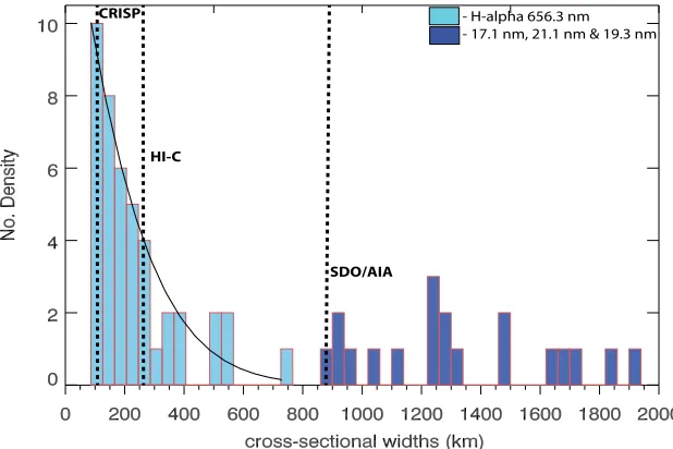
CRISP - H-alpha 656.3 nm - 17.1 nm, 21.1 nm & 19.3 nm

HI-C

SDO/AIA

Figure 10.Histogram displaying the distribution of all detectable strands and substructures within coincident Hαand EUV coronal loops, as measured from all of the data sets sampled. The pale blue sections correspond to the Hα-only detections made via CRISP. The darker blue sections correspond to theSDO/AIA coronal loop cross-sections. The vertical dashed lines mark the resolution limit for CRISP, Hi-C, andSDO/AIA. The number density of detected strands vs. their cross-sectional FWHM widths is measured. The exponential curve is overlaid onto the plot to indicate the steeping distribution toward finer scales within the substructures of coronal loops.

(A color version of this figure is available in the online journal.)

continuous detectable strand (which largely features close to the resolution limit in CRISP at 130 km) was on the order of 26,100 km, extending from loop-top to close to the footpoint. This represents one of the longest and continuous fine-scale coronal loop substructures detected to date.

Antolin et al. (2010) observed coronal rain near coronal loop-tops withHinode(SOT; Tsuneta et al.2008) and measured cross-sectional widths on the order of 500 km. We detect similarly scaled coronal rain strands in coronal loop-tops with CRISP and also threads with finer scales, implying the existence of a range of finely scaled structures in the outer solar atmosphere. The draining of the dense plasma as it falls back toward the loop footpoints from the loop-top is most clear in data set C, represented in Figures8and9. In the images, we demonstrate a clear association of the rain flowing within both legs of a post-flare coronal loop from its apparent source near the loop-top. There appears to be a distribution of scales within the coronal loop-top with respect to cross-sectional widths of strands. Likewise, there is a distribution in the strand lengths, all of which appear to follow the trajectory of the loop-top coronal field (as inferred from co-incident AIA loop trajectories), with some appearing to be very much extended toward the loop footpoint. This shows that the fine-scale structure is widespread along the full length of the loop and that the coronal rain clumps can form within bunches of strands. We can conclude that the vast majority of fine-scale strand structures within coronal loop cross-sections exist well below the resolution of SDO/AIA (69.3% of the potential strands, as returned by CRISP, are unresolved with AIA), and almost 50% of fine-scale strands could potentially remain unresolved with imaging in an instrumental resolution comparable to Hi-C. In summary, after considering eight cross-cuts (representing one loop-top and two loop-legs for data sets B and C and one loop-top and one loop-leg for data set A) we find an average ratio of 5:2 for CRISP strand number density to AIA strand number density per loop system. Finally, we conclude that there is a cutoff in the peak of the distribution (from Figure10) at the instrumental resolution

of CRISP. We and others have assumed that the distribution of strand sizes should be a Gaussian or at least symmetric about some peak. From our histogram, we demonstrate that either we have not yet reached that peak and the actual fine-scale resolution is much below 100 km, or the spatial-fine-scale distribution is in fact skewed away from being symmetric about some peak. This result clearly states that even with the most powerful ground-based instrumentation available, we have not yet observed a true peak in the strand cross-sectional width measurements at the lowest limit within coronal loops. Fang et al. (2013) demonstrated with numerical simulations of coronal rain formation that when compared with observational statistics, a higher percentage of coronal rain clumps are expected in smaller scales. Here, we can confidently state that the peak (in other words the minimum) in cross-sectional width distribution of the finest structures within coronal loops is most likely to exist beneath the 100 km mark. Henceforth, we look forward with great anticipation to the arrival of more powerful ground-based telescope facilities (such as the 4 m Daniel K. Inouye Solar Telescope (Berger & ATST Science Team2013) in order to fully probe even finer scales within coronal loop cross-sections.

Eamon Scullion currently a Government of Ireland Postdoc-toral Research Fellow supported by the Irish Research Coun-cil (Project ID:GOIPD/2013/308). We thank N Frej who co-observed the mosaic and 2010 July 1 data sets (A and B), as well as A. O. Carbonell and B. Hole, who observed at the SST on the 2011 September 24 data set (C). The Swedish 1 m Solar Telescope is operated on the island of La Palma by the Insti-tute for Solar Physics of Stockholm University in the Spanish Observatorio del Roque de los Muchachos of the Instituto de Astrofisica de Canarias.

REFERENCES

The Astrophysical Journal, 797:36 (10pp), 2014 December 10 Scullion et al.

Antolin, P., Vissers, G., & Rouppe van der Voort, L. 2012, SoPh, 280, 457

Aschwanden, M. J. 2004, Physics of the Solar Corona. An Introduction (Chichester, UK: Praxis Publishing Ltd)

Berger, T. ATST Science Team. 2013, BAAS, 44, 400.02

Beveridge, C., Longcope, D. W., & Priest, E. R. 2003, SoPh,216, 27 Bray, R. J., Cram, L. E., Durrant, C., & Loughhead, R. E. 1991, Plasma Loops

in the Solar Corona (Cambridge: Cambridge Univ. Press) Brooks, D. H., Warren, H. P., & Ugarte-Urra, I. 2012,ApJL,755, L33 Brooks, D. H., Warren, H. P., Ugarte-Urra, I., & Winebarger, A. R. 2013,ApJL,

772, L19

Cargill, P. J. 1994,ApJ,422, 381

Cargill, P. J., & Klimchuk, J. A. 2004,ApJ,605, 911

Cirtain, J. W., Golub, L., Winebarger, A. R., et al. 2013,Natur,493, 501 Culhane, J. L., Harra, L. K., James, A. M., et al. 2007, SoPh,243, 19 De Groof, A., Berghmans, D., van Driel-Gesztelyi, L., & Poedts, S. 2004,A&A,

415, 1141

de la Cruz Rodr´ıguez, J., L¨ofdahl, M., S¨utterlin, P., Hillberg, T., & Rouppe van der Voort, L. 2014, A&A, in press (arXiv:1406.0202)

DeForest, C. E. 2007,ApJ,661, 532

Fang, X., Xia, C., & Keppens, R. 2013,ApJL,771, L29

Gomez, D. O., Martens, P. C. H., & Golub, L. 1993,ApJ,405, 767 Henriques, V. M. J. 2012,A&A,548, A114

Kawaguchi, I. 1970, PASJ,22, 405 Klimchuk, J. A. 2000,SoPh,193, 53

Klimchuk, J. A. 2006,SoPh,234, 41

Klimchuk, J. A., & Cargill, P. J. 2001,ApJ,553, 440

Klimchuk, J. A., Patsourakos, S., & Cargill, P. J. 2008,ApJ,682, 1351 Kosugi, T., Matsuzaki, K., Sakao, T., et al. 2007,SoPh,243, 3

Leenaarts, J., Carlsson, M., & Rouppe van der Voort, L. 2012,ApJ,749, 136 Lemen, J. R., Title, A. M., Akin, D. J., et al. 2012, SoPh,275, 17

Peter, H., Bingert, S., Klimchuk, J. A., et al. 2013,A&A,556, A104 Reale, F. 2010, LRSP,7, 5

Reale, F., Nigro, G., Malara, F., Peres, G., & Veltri, P. 2005,ApJ,633, 489 Scharmer, G. B. 2006,A&A,447, 1111

Scharmer, G. B., Bjelksjo, K., Korhonen, T. K., Lindberg, B., & Petterson, B. 2003a,Proc. SPIE,4853, 341

Scharmer, G. B., Dettori, P. M., Lofdahl, M. G., & Shand, M. 2003b,Proc. SPIE,4853, 370

Scharmer, G. B., Narayan, G., Hillberg, T., et al. 2008,ApJL,689, L69 Schrijver, C. J. 2001, SoPh,198, 325

Sekse, D. H., Rouppe van der Voort, L., De Pontieu, B., & Scullion, E. 2013,ApJ, 769, 44

Tsuneta, S., Ichimoto, K., Katsukawa, Y., et al. 2008, SoPh,249, 167 Ugarte-Urra, I., Brooks, D. H., & Warren, H. P. 2012, BAAS, 220, 309.03 van Noort, M., Rouppe van der Voort, L., & L¨ofdahl, M. G. 2005, SoPh,

228, 191

van Noort, M. J., & Rouppe van der Voort, L. H. M. 2008,A&A,489, 429 Vissers, G., & Rouppe van der Voort, L. 2012,ApJ,750, 22