Accepted Manuscript
Information demand and stock return predictability
Dimitris K. Chronopoulos, Fotios I. Papadimitriou, Nikolaos Vlastakis
PII: S0261-5606(17)30191-2
DOI: https://doi.org/10.1016/j.jimonfin.2017.10.001
Reference: JIMF 1847
To appear in: Journal of International Money and Finance
Please cite this article as: D.K. Chronopoulos, F.I. Papadimitriou, N. Vlastakis, Information demand and stock return predictability, Journal of International Money and Finance (2017), doi: https://doi.org/10.1016/j.jimonfin. 2017.10.001
1
Information demand and stock return predictability
Dimitris K. Chronopoulos
†School of Management, University of St Andrews, St Andrews, KY16 9RJ, Scotland, UK
Fotios I. Papadimitriou
Southampton Business School, University of Southampton, Southampton, SO17 1BJ, UK
Nikolaos Vlastakis
Essex Business School, University of Essex Wivenhoe Park, Colchester, CO4 3SQ, UK
Tel: (+44) (0) 1206 874591 [email protected]
Abstract
Recent theoretical work suggests that signs of asset returns are predictable given that their volatilities are. This paper investigates this conjecture using information demand, approximated by the daily internet search volume index (SVI) from Google. Our results reveal that incorporating the SVI variable in various GARCH family models significantly improves volatility forecasts. Moreover, we demonstrate that the sign of stock returns is predictable contrary to the levels, where predictability has proven elusive in the US context. Finally, we provide novel evidence on the economic value of sign predictability and show that investors can form profitable investment strategies using the SVI.
JEL Classification: G11, G14, G17
Keywords: Return sign predictability, Information demand, Investor attention, Volatility forecast, Economic value
1
Information demand and stock return predictability
Abstract
Recent theoretical work suggests that signs of asset returns are predictable given that their volatilities are. This paper investigates this conjecture using information demand, approximated by the daily internet search volume index (SVI) from Google. Our results reveal that incorporating the SVI variable in various GARCH family models significantly improves volatility forecasts. Moreover, we demonstrate that the sign of stock returns is predictable contrary to the levels, where predictability has proven elusive in the US context. Finally, we provide novel evidence on the economic value of sign predictability and show that investors can form profitable investment strategies using the SVI.
JEL Classification: G11, G14, G17
2
1. Introduction
The question of whether stock market returns contain a predictable component has attracted
much attention from both academics and market participants. As a result, numerous financial
and macroeconomic variables have been employed to address the issue (see, inter alia,
Rozeff, 1984; Campbell and Shiller, 1988; Fama and French, 1988; Hodrick, 1992; Lamont,
1998; Pontiff and Schall, 1998; Lettau and Ludvigson, 2001; Boudoukh et al., 2006; Kellard
et al., 2010; Andriosopoulos et al., 2014; Jordan et al., 2014) while a plethora of approaches
and testing procedures have emerged in the literature making the overall assessment an
extremely difficult task (e.g., Goetzmann and Jorion, 1993; Nelson and Kim, 1993; Ferson et
al., 2003; Inoue and Kilian, 2004; Amihud and Hurvich, 2004; Lewellen, 2004).1
However, although the empirical evidence on return predictability is mixed when we
consider stock returns in the levels, there is a smaller body of literature which suggests that it
is more likely to predict the signs of stock returns instead (see, Breen et al., 1989; Pesaran
and Timmermann, 1995, 2000; Christoffersen et al., 2007; Nyberg, 2011; Chevapatrakul,
2013). An important development in this area is the recent theoretical work by Christoffersen
and Diebold (2006) which suggests that the sign of stock returns is predictable given that
their volatilities are.2 The intuition behind this relationship is that any changes in volatility
will alter the probability of observing negative or positive returns. More specifically, a rise in
volatility increases the probability of a negative return, given that the expected returns are
positive. Christoffersen and Diebold (2006) point out that sign predictability may exist even
if there is no mean predictability, while it is also independent of the shape of the return
distribution. Such sign predictability can be particularly useful for creating profitable
investment strategies.
Building on the work of Christoffersen and Diebold (2006), which provides a more
concrete framework for sign predictability, we empirically investigate whether improved
volatility forecasts, via a measure for information demand, can indeed lead to better sign
forecasts of stock returns. Given that stock return predictability in the levels has been proven
difficult to detect in the US context (see, Bossaerts and Hillion, 1999; Goyal and Welch,
2003, 2008, Kostakis et al. 2015), it is of particular interest to investigate whether the sign of
US stock returns can be predicted instead. Additionally, we investigate whether such sign
return predictions can be exploited to form profitable trading strategies from the perspective
1
For a comprehensive and up-to-date overview of stock return predictability, see Rapach and Zhou (2013).
2
3 of investors. This is important for two reasons. First, statistical significance does not
necessarily translate into economic gains for investors (Leitch and Tanner, 1991;
Andriosopoulos et al., 2014) and second, apart from the theoretical contribution of
Christoffersen and Diebold (2006), there is no empirical evidence regarding the economic
value of sign predictability based on their model.
To achieve our goal, we turn to the link between return volatility and information
flow. As suggested by Ross (1989), the return volatility is directly related to the rate of flow
of information to the market. Hence, information about an event occurring (i.e. a signal) will
affect the volatility of stock returns and more so if the informational content of this event is
low (Gerlach, 2005; Li, 2005). In this case, the demand for information will increase up to the
point that the prevailing ambiguity about the state of the world is resolved (Moscarini and
Smith, 2002). In other words, the demand for information about an event is directly related to
the “quality” of a signal, which is in turn related to return volatility. In a recent study,
Vlastakis and Markellos (2012) construct a proxy for demand for information based on the
internet “Search Volume Index” (SVI henceforth) from Google. Their analysis reveals a
positive and significant contemporaneous relationship between the SVI and historical (and
implied) measures of volatility in the US market. Vlastakis and Markellos (2012) also argue
that in the networked world information discovery is shared between traditional information
providers (such as those employed by sophisticated investors, e.g. Reuters) and alternative
channels on the internet. It follows that information arrives on average at roughly the same
time for both institutional and retail investors. Therefore, SVI captures the reaction of retail
investors to the same signals that institutional investors observe and react to. Consequently,
we expect that the use of the SVI as a measure for demand for information can lead to better
volatility forecasts. To this end, we augment a number of GARCH family models with the
daily SVI to construct better volatility forecasts. Subsequently, we obtain sign forecasts using
the model of Christoffersen and Diebold (2006) which we compare against forecasts from
various other competing models. Moreover, based on the produced sign forecasts we
formulate appropriate trading strategies and examine whether a real-time investor would be
able to exploit any sign predictability. Specifically, we adopt the framework of Granger and
Pesaran (2000) and consider an investor who, at each period, has the option to invest her
wealth either in stocks or in bonds. Therefore, in a dynamic setting, the investor maximizes
her utility function using a time-varying optimal predictive rule to translate sign probability
4 & Poor’s 500 (S&P 500) index and spans the period from January 2, 2004 through December
31, 2016.
Our contribution to the literature is threefold. First, we show that the most prominent
candidate to predict the sign of daily stock returns is the model suggested by Christoffersen
and Diebold (2006) when extended with the SVI variable. Specifically, we find that it
outperforms all considered types of competing models either in their standard form or
extended with a number of variables which have been shown to work well in previous studies
on asset pricing and asset return sign forecasts. For instance, based on the Brier score which
is a commonly used scoring rule to evaluate probability forecasts, it produces on average
2.6% more accurate return sign forecasts compared to a naive model which only considers
the proportion of positive past returns. This finding highlights the usefulness of the demand
for information measure (SVI) in predicting the sign of US stock returns. This is a novel
finding in the return predictability literature which is robust to different sample periods (both
normal and volatile) and further confirmed by the Diebold and Mariano (1995) test statistic of
equal predictive accuracy.
Second, our study offers evidence which suggests that the model by Christoffersen
and Diebold (2006) exhibits a good performance in terms of economic value. Moreover, we
show that the inclusion of the SVI variable can enhance this model and lead to even higher
economic gains for investors. This is the first study to confirm the efficacy of the
aforementioned model for real-time investors and to also suggest a new variable that further
improves its performance. For example, we find that an active trading strategy that utilises
the SVI variable within the Christoffersen and Diebold (2006) framework produces a higher
return and a lower standard deviation, which results in a higher Sharpe ratio compared to a
simple buy and hold strategy. Our results in this context are robust to different utility
functions, levels of risk aversion and estimates of transaction costs. Furthermore, our
conclusions remain unaffected under different realistic scenarios (with or without short-sales)
and measures of economic value. Third, we demonstrate that the inclusion of the SVI variable
in all considered GARCH family models leads to superior stock market volatility forecasts.
This finding extends an emerging literature which establishes a relationship between
measures of demand for information and asset return volatility (e.g., Vlastakis and Markellos,
2012; Andrei and Hasler, 2014; Vozlyublennaia, 2014; Da et al., 2015; Dimpfl and Jank,
2015; Goddard et al., 2015).
Overall, this study answers calls for research on formulating strategies and assessing
5 complements the literature by providing new empirical evidence on how investors’ attention
and reaction to new information can enhance the predictability of asset return signs.
The paper is organised as follows. Section 2 provides a description of our data and the
variables used in our study. Section 3 presents the methodological approach and Section 4
discusses the empirical findings. Finally, Section 5 concludes.
2. Data
This paper employs data at a daily frequency covering the period from January 2, 2004 to
December 31, 2016. Our sample size is determined by the data availability of our main
predictive variable of interest, namely the demand for information which is discussed below.
In more detail, we use daily prices of the S&P 500 index obtained from the Center for
Research in Security Prices (CRSP). The monthly Treasury bill rate, which proxies for the
risk-free rate, is from Ibbotson and Associates and it is available from Kenneth French’s
website. As in Pesaran and Timmermann (1995) and Chevapatrakul (2013), the excess
returns on the stock market, , are computed as , where is
the closing price of the S&P 500 index and is the return from holding a one-month
Treasury bill over the period from t 1 to t.
To capture the demand for information we follow Vlastakis and Markellos (2012) and
use a proxy for information flow based on the number of searches on Google. Specifically,
we use the SVI which represents the total searches for any keyword on Google in the form of
an index, so that the observation with the highest number of searches in a given sample takes
the value of 100.
Our main forecasting variable is the change in the SVI, defined as . Given that our goal is to predict the direction of change of the S&P 500 index, the
term used as a search keyword is “s&p 500”. The selection of this term was decided through
a procedure similar to the one followed by Vlastakis and Markellos (2012) and entails
inserting the full name of the stock index and checking all similar terms suggested by Google
Trends as well as Wordtracker. We finally opted for the term that was the least ambiguous
and had the highest search volume.3 Google offers data on the SVI from January 2004
onwards, thus leaving us with 3,263 daily observations. A description of the process we
follow to obtain a consistent daily time-series of SVI is provided in the Appendix.
3
6 In order to assess the accuracy of volatility forecasts we need to compare them against
the true volatility. However, volatility is a latent variable which cannot be directly observed
and hence a proxy for it is required. For this purpose we use realized volatility ( ) based on
5 minute returns with subsampling obtained from the Realized Library of the Oxford-Man
Institute.
Moreover, a number of other variables are relevant to the study. Specifically, we use
two different bond yields, namely, the short-term bond yield ( ) and the long-term bond
yield ( ). The former is measured by the yield of the 3-month Treasury bill, while the latter
is measured by the yield of the 10-year Treasury bond. Finally, we also use a bond yield
spread, namely, the slope of the Treasury yield curve ( ), which is defined as the
difference between the yields on the 10-year and the 3-month Treasury securities. The data
on the bond yields are obtained from the St. Louis FED’s FRED database.
Table 1 presents descriptive statistics of all variables considered in our study. As
reflected by the high levels of skewness and kurtosis, all variables display a significant
departure from normality. However, as shown in Christoffersen and Diebold (2006), the
theoretical result that volatility forecastability implies sign forecastability holds even if
returns do not follow a Gaussian distribution. Additionally, as mentioned in Christoffersen et
al. (2007), if the distribution is asymmetric then the sign can be predictable even if the
expected return is zero. Therefore, there is no concern regarding whether the empirical results
in our paper can be affected by the evidence of non-normality in the return series. Turning to
ΔSVI, we find that it is positively skewed with excess probability in the tails, as suggested by
the higher moments. Moreover, it has a negative autocorrelation of -0.33. Finally, the
stationarity of ΔSVI is assessed using three unit root tests: the Augmented Dickey-Fuller test
(ADF, Dickey and Fuller, 1979), the Phillips-Perron test (PP, Phillips and Perron, 1988), and
the Kwiatkowski, Phillips, Schmidt, and Shin test (KPSS, Kwiatkowski et al., 1992).
Whereas for the ADF and PP tests the null hypothesis is the existence of a unit root in the
data, the null hypothesis for the KPSS test is stationarity. The corresponding statistics are,
respectively, -30.811, -392.260 and 0.4384 and suggest that the ΔSVI is stationary.
[Insert Table 1 around here]
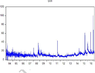
For completeness, Figure 1 shows the graph of the SVI variable. As can be seen from
the graph, demand for information abruptly increases in October and November 2008 after
Lehman’s bankruptcy. Furthermore, demand for information also spikes on August 8, 2011
7 sovereign debt and on June 24, 2016 when the UK voted in favour of exiting the EU. Finally,
it reaches a record level on November 9, 2016 when the new US president was elected.
Overall, the graph indicates that SVI is associated with demand for information related to the
market.
[Insert Figure 1 around here]
3. Methodology
3.1. The framework of return sign predictability
Christoffersen and Diebold (2006) demonstrate that the sign of asset returns can be
predictable even if the expected returns are not, provided that their volatility is. To see this,
let denote a series of excess returns, which follows a distribution that depends only on its
first two moments, and let be the information set available at time . Moreover, the
conditional mean and variance of the expected excess returns are denoted, respectively, by
and . If varies with we say that the
return series displays conditional mean dependence and hence it is predictable. Similarly, if
varies with , we can define conditional variance dependence (or volatility
predictability). If the probability of a positive return at time t also varies with then the
sign of the return series is predictable. In this case, the conditional probability of a positive
excess return is given by:
, (1)
where is the cumulative distribution function of the standardized return
. Provided that the conditional volatility is predictable, the sign of the
return will also be predictable even if the expected excess return is constant over time but
different from zero (i.e. and ). This is because, as equation (1) suggests, the
probability of a positive return is time varying as volatility moves.4
Building on the above framework, and with the aim to provide fresh empirical
evidence, in this paper we forecast the probability of observing a positive excess return on the
4
As mentioned earlier, even if the sign of the excess return will continue to be predictable provided
8 S&P 500 index using forecasts of its expected excess returns as well as its volatility. The
methodological approach for obtaining such forecasts is discussed below.
3.2. Volatility forecasting models
As suggested by the work of Christoffersen and Diebold (2006), forecasting the daily stock
market return volatility plays a key part in predicting accurately the sign of stock market
returns. Therefore, we turn to the GARCH family models that have been shown to perform
well in forecasting conditional stock return volatility (Poon and Granger, 2003). These
models involve the joint estimation of a conditional mean and a conditional variance
equation. The return process is assumed to be generated as:
, (2)
where is the excess return and is the error term. The GARCH (1,1) process
introduced by Bollerslev (1986) and Taylor (1986) is given by:
, (3)
where ensures the positiveness of the conditional variance. For the
unconditional variance to exist, a necessary and sufficient condition is that .
As stressed earlier, one of the main objectives of our study is to examine whether
investors’ demand for information can improve volatility forecasts. Hence, we extend the
standard GARCH (1,1) model to a GARCH-SVI (1,1) model by incorporating the Google
SVI index both in the mean and in the variance equations as follows:
, (4)
, (5)
where ΔSVI is the change in the demand for information.
We also consider popular extensions of the basic GARCH model. One such extension
is the GJR due to Glosten et al. (1993) which accommodates the asymmetry in the response
of volatility to positive and negative shocks. The conditional variance in the GJR-GARCH
model has the following form:
, (6)
where if and if .
Similarly to the GARCH model, we also extend the GJR-GARCH to include the ΔSVI
variable as follows:
, (7)
9 In addition, we employ the EGARCH model proposed by Nelson (1991) which,
unlike the GARCH (1,1) model, does not require imposing non-negativity constraints.
Moreover, similar to the GJR-GARCH, the standard EGARCH model does not enforce a
symmetric response of volatility to positive and negative shocks. The EGARCH (1,1)
specification can be expressed as follows:
. (9)
As with the other volatility models, we extend the EGARCH (1,1) specification by including
the demand for information proxy variable. The relevant EGARCH-SVI (1,1) model is then
written as:
, (10)
. (11)
To obtain one-step-ahead forecasts of the conditional volatility, we rely on a recursive
scheme. Let denote the full sample size where L is the number of in-sample
observations and P is the number of out-of-sample forecasts. For all models, we initially use
the first observations to get the corresponding set of parameter estimates. The first
one-step-ahead forecast error is then constructed by comparing our forecasted volatility against
the realised volatility, which serves as a proxy of the latent return volatility. In order to
construct the second one-step-ahead forecast error, we use data available through period
and repeat the above procedure. This process continues until all observations are used
and we have a sequence of one-step-ahead ahead forecast errors.
We report the statistics of the out-of-sample forecast errors obtained in different
sample periods. In particular we document the mean, standard deviation, and root mean
square error (RMSE) of volatility forecast errors resulting from each competing model
presented above. The parameters are estimated by Quasi Maximum Likelihood using a
Gaussian Likelihood.
3.3. Assessing volatility forecasts
One issue when comparing volatility forecasts is that the model with the smallest forecast
error is not necessarily superior to the other competing models. Hence, we need to formally
10 statistical sense. For this purpose, we employ the Diebold and Mariano (1995) (DM) statistic
which tests for equal predictive accuracy. In particular, Diebold and Mariano (1995) suggest
the use of a t-statistic for pairwise model comparisons in terms of forecasting performance.
Their approach involves taking the loss differential between two competing models scaled by
a robust estimator of its variance and comparing it against the standard normal distribution.
When comparing forecasts between non-nested models, such as between the GARCH
model against the EGARCH model, the DM statistic has a standard normal distribution (see
West, 1996). However, when comparing forecasts from nested models McCracken (2007)
shows that the DM statistic has a non-standard limiting distribution and provides
asymptotically valid critical values for various combinations of in-sample and out-of-sample
proportions. For instance, in our study this case applies when we compare forecasts between
a standard form GARCH family model and its extended counterpart (e.g., EGARCH and
EGARCH-SVI).
3.4. Return sign forecasting models
To estimate the probability of a positive return on the S&P 500 index we adopt the
framework by Christoffersen and Diebold (2006) (C&D) and Christoffersen et al. (2007) and
employ a model which allows for the forecasted probability to be conditioned on the
predictive variable of interest through volatility forecasts. Based on the relevant model,
shown in equation (12) below, the t +1 period forecast is generated as:
, (12)
where is the indicator function, is the one-step-ahead volatility forecast as
described above, and is the one-step-ahead expected return forecast. The is
estimated as an AR(1) process. As explained earlier, in this paper we use the change in the
demand for information to enhance the volatility forecasts of the S&P 500 index returns.
Therefore, we extend the C&D model by incorporating the ΔSVI variable both in , as
described in Section 3.2, and in .
The probability forecasts from our main model (C&D-SVI) are then compared against
those generated by a naive model as well as by a number of alternative models which have
been previously used to predict the sign of stock returns. In particular, one-step-ahead
probability forecasts from the naive model are generated as follows:
11 That is, our naive model is based on the empirical distribution function of the return. In other
words, we consider the proportion of positive past returns from the beginning of the sample
period up to the time the forecast is made. To further assess the robustness of our main
model, we also employ some alternative competing models which have been used in the
extant literature to construct probability forecasts. Specifically, we consider a dynamic probit
model (see, Nyberg, 2011) which uses a binary sign return indicator as the dependent variable
and also accounts for potential autocorrelation in the structure of the return signs time series.
Based on this model, probability forecasts are constructed as shown in equation(14):
. (14)
Moreover, similar to Nyberg (2011) and Chevapatrakul (2013), we consider a number of
alternative specifications of the dynamic probit model in equation (14) which control for
various factors that have been used to predict return signs. Specifically, we employ three
models which extend the dynamic probit model by adding, respectively, the short term yield,
, the long term yield, , and the term spread, , as in equation (15) below:
, (15)
where Z can be one of the variables, , or , as discussed above. Finally, we also
consider a dynamic probit model (DynProbit-All) which incorporates all three variables
mentioned above.
To compare the predictive performance of each model we report statistics on the
out-of-sample prediction errors obtained in different sample periods. In particular, we document
the mean, standard deviation and Brier scores of the probabilistic forecast errors derived from
each model. The Brier score is a commonly used scoring rule to evaluate probability forecasts
(Brier, 1950). It may be viewed as the mean squared loss function for probabilistic forecasts.
The Brier score for a sample of binary forecasts, where the event either occurs or does not
occur, is given by , where is the predicted probability of the
event occurring according to the tth forecast, and is equal to one or zero, depending on
whether the event actually occurs or not. To assess whether any identified differences
between the competing models are also statistically significant we employ the DM statistic as
in the case of comparing volatility forecasts (see section 3.3).
4. Empirical results
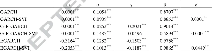
12 Table 2 presents the estimates of the different standard GARCH model specifications
employed in our study as well as their extended with the ΔSVI counterparts. These in-sample
results indicate that the coefficient of ΔSVI is positive and statistically significant across all
different GARCH models.5 This finding suggests that ΔSVI possesses significant in-sample
predictive power for return volatility and enriches standard GARCH models with useful
information about market variation. Moreover, the coefficient γ is also found to be significant
in both the GJR-GARCH and EGARCH models suggesting the existence of asymmetry in the
conditional return distribution. As suggested by Christoffersen et al., (2007) such evidence of
asymmetry implies that the sign of returns could be predictable provided that their volatility
is. Overall, these results extend an emerging literature which establishes a relationship
between measures of demand for information and asset return volatility (e.g., Vlastakis and
Markellos, 2012; Andrei and Hasler, 2014; Vozlyublennaia, 2014; Da et al., 2015; Dimpfl
and Jank, 2015; Goddard et al., 2015).
[Insert Table 2 around here]
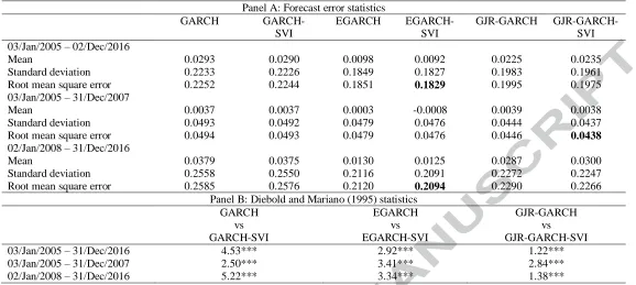
Panel A in Table 3 tabulates the forecast error statistics obtained from the volatility
models described in Section 3.2 which are employed to produce one-step-ahead
out-of-sample daily forecasts of the S&P 500 return volatility. To allow for a more thorough
examination of forecasting performance, the computed statistics are also reported for two
different sub-sample periods. The first sub-sample spans the period from January 3, 2005 to
December 31, 2007 whereas the second one covers the period from January 2, 2008 to
December 31, 2016 which includes the recent financial crisis.
[Insert Table 3 around here]
Panel A reveals that the inclusion of the ΔSVI variable in all considered volatility
models improves their out-of-sample forecasting ability as indicated by the reported RMSEs.
This result is robust not only across all model specifications but also in all sample periods
under consideration. This is a new finding in the literature which indicates that the change in
demand for information conveys additional useful information and enhances daily forecasts
of stock return volatility.6
5
As a robustness check, we also estimated the considered GARCH models by additionally including either the VIX2, the realised volatility or the trading volume. In all cases, ΔSVI remains significant and its coefficient maintains the correct sign. To account for potential multicollinearity problems, we follow Cooper and Priestley (2009) and Andriosopoulos et al. (2014) and we look at the relative performance of ΔSVI and the VIX2 (Realised Volatility or Trading Volume), when the latter is orthogonalised relative to the former.
6
13 On the other hand, if we compare volatility forecasts derived from the GARCH model
against those derived from the asymmetric GARCH family models, we observe that the latter
exhibit a superior forecasting performance. Specifically, the EGARCH-SVI model exhibits
the best forecasting performance, as suggested by the smallest RMSE, followed by the
standard EGARCH model. These results are consistent with the study by Awartani and
Corradi (2005) who also report that asymmetric GARCH models lead to better volatility
forecasts relative to their symmetric counterparts.
The identified RMSE differences discussed above do not necessarily suggest that the
competing models produce forecasts which are also different in a statistical sense. Therefore,
we need to formally examine whether the inclusion of the ΔSVI variable in our volatility
models can indeed lead to significantly better forecasts. To this end, we conduct a test of
equal predictive accuracy. As such, Panel B in Table 3 tabulates the computed DM statistics
when we compare each volatility model against its extended with the ΔSVI variable
counterpart across different periods. The DM statistics suggest that the inclusion of the ΔSVI
variable significantly improves the predictive power of all GARCH family models at the 1%
level during the full out-of-sample period. This result is robust across all considered periods
and establishes that the ΔSVI contains valuable information for predicting stock market
volatility.
4.2. Sign predictability results
Given that the EGARCH-SVI and the EGARCH models produce the best volatility forecasts
among all competing models under consideration, we now further explore whether we can
exploit these forecasts to achieve better sign predictability of daily stock returns as suggested
by Christoffersen and Diebold (2006).7 Using both of these volatility models will also allow
us to empirically assess i) how the C&D model compares against other types of models that
are relevant for sign predictability and ii) whether the extension we propose in this paper with
the ΔSVI variable can enhance the sign forecasting power of the C&D model. Panel A in
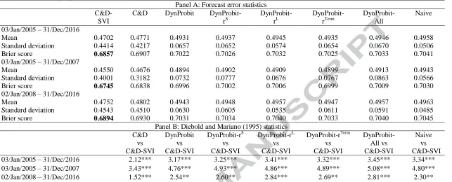
Table 4 shows the forecast error statistics derived from all models described in Section 3.4
which are used for return sign predictability. As in the case of volatility forecasts, these
volatility forecasting power and additionally, none of these models (either standard or extended) outperform the EGARCH-SVI model or the simple EGARCH model. Therefore, based on the theory put forward by Christoffersen and Diebold (2006), we consider only these two volatility models when constructing return sign forecasts.
7
14 statistics are also reported for two different sub-sample periods (one of which includes the
recent financial crisis).
[Insert Table 4 around here]
Based on the produced Brier scores, the results suggest that the model by
Christoffersen and Diebold (2006) extended with the ΔSVI variable is the most prominent
candidate for predicting the sign of daily stock returns. Specifically, it outperforms all other
competing models, either in their standard form or enhanced with a number of variables
which have been shown to be relevant for asset return and sign forecasts. This finding is
consistent across all periods and is further confirmed by means of the DM statistic (see Panel
B of Table 4). It is worth mentioning here that none of the extended dynamic probit models
considered in the analysis manages to outperform the baseline dynamic probit model
(DynProbit). This finding is broadly in contrast to recent evidence which suggests that
variables such as the short term interest rate and the long term interest rate perform well when
monthly data are considered (Nyberg, 2011; Chevapatrakul, 2013). Hence, our findings point
to the direction that the ΔSVI seems to convey more useful information for predicting the
sign of returns at higher frequencies.
To shed more light on our findings, we further explore whether this sign predictability
is driven by predictability in the mean or in the variance. To this end, we estimate Equation
(4) and we find that the lagged ΔSVI is not a significant in-sample predictor of stock returns
at the level. This result indicates that predictability in the variance drives sign predictability
of returns in our sample. This is consistent with the theory of Christoffersen and Diebold
(2006) which suggests that sign predictability can exist independently of mean predictability.
4.3. Further analysis of sign predictability: economic significance
Finding statistical significance in terms of predictive ability is neither a necessary nor a
sufficient condition for a profitable investment strategy (Leitch and Tanner, 1991; Diebold
and Lopez, 1996). Therefore, in this section we explore whether sign forecasts can help
improve investor’s decisions and lead to a profitable investment strategy. In particular, we
consider an investor with a utility function for wealth w defined as , where A
is the investor’s degree of risk aversion.8 As in Goetzman et al. (2007), Della Corte et al.
(2010), and Andriosopoulos et al. (2014), we assume that the risk aversion coefficient is
8
15 three.9 The investor has the option to invest either in the S&P 500 index or in a riskless asset
(treasury bills) assuming that sales and purchases of stocks and bonds are subject to
transaction costs. The investment decision is then based on the probability of observing a
positive return on the index in the next period as generated by each of the predictive models
discussed in Section 3.4. To provide a more comprehensive examination of economic value
we consider both scenarios where short sales are either allowed or prohibited. Therefore, our
paper is relevant to investors operating under different constraints.
4.3.1. The framework for measuring economic significance
In order to assess the economic value of return sign forecasts, we adopt the decision-theoretic
framework put forward by Granger and Pesaran (2000). Within this framework, a utility
maximising investor considers the utility of both successful and failed predictions of an
upward movement in the stock index before taking action. Let be an
indicator of the realised direction of the return on the S&P 500 index and be the
corresponding directional forecast. Then the investor tries to maximise the following utility
function:
, (16)
where is the utility when and with . We also assume that
the utility of a correct prediction is always greater than that of a false prediction. That is
and . Moreover, let denote the forecasted probability of an
upward movement for the S&P 500 index formed at the beginning of the period . Under the
above set up the expected utility of taking action is given by , while
the expected utility of not taking action is given by . Therefore, the
maximizing utility investor will make the prediction if:
(17)
or
. (18)
9
16 In our paper, we consider two alternative scenarios. The first scenario is more restrictive and
does not allow for short-sales while under the second scenario short-sales are allowed. In the
case of the first scenario we have the following:
(19)
where represents the portfolio weight attributed to the stock market index. The realised
return from the active trading strategy is then given by:
, (20)
where is the return on the S&P 500 index and denotes the return on the riskless
asset. In this setup the investor may decide to fully invest either in treasury bills that yield
or in the S&P 500 index, which yields in the event of a market rise and
in the event of a market fall. Following Granger and Pesaran (2000), historical averages of
positive and negative index returns of up to time t are used to predict and ,
respectively. In our analysis we also consider transaction costs for stocks and bonds which
are denoted by and respectively. The payoff matrix for this scenario is described in
Table 5.
[Insert Table 5 around here]
Based on Table 5 and assuming the investor is fully invested in the risk-free asset she will
switch to the stock index (i.e. ) if:
, (21)
where . Now, if the investor is fully invested in the stock index she will
switch to the risk-free asset (i.e. ) only if:
. (22)
Finally, she will remain inactive if .
Regarding the second scenario of our economic analysis, we follow Campbell and
Thompson (2008) and Maio (2013) and we extend the strategy presented above to allow for
the possibility of short-selling the stock index. Based on this scenario, the investor can exploit
further her predictions for stock market movements and potentially achieve higher economic
gains. The corresponding weights for this strategy are now given by:
17 Therefore, the investor will allocate 150% of her wealth to the stock index in case of a
positive return prediction, borrowing 50% at the risk-free rate. In case of a negative return
prediction she will sell short the stock index at 100% and invest the proceeds in the risk- free
asset.10 The relevant payoff matrix based on these weights is described in Table 6.
[Insert table 6 around here]
As can be seen in Table 6, the investor will go long on the index if:
,
(24)
whereas she will sell short the index if:
. (25)
As before, she will remain inactive if .
The optimal predictor that maximizes the expected utility of the investor under either
scenario is given by:
, (26)
where , and .
Under both scenarios presented above the return of each active strategy is compared
against the return of a passive “buy-and-hold” (B&H) strategy which goes 100% long on the
stock index throughout the investment horizon. To further evaluate the economic
performance of each active strategy and to be comparable with related studies we initially
employ the commonly used Sharpe ratio. We then compare all Sharpe ratios against the
corresponding Sharpe ratio obtained from the passive B&H strategy. This is important since
different strategies might involve different levels of risk. As a further check, we test whether
the Sharpe ratio of any active trading strategy is also statistically different from the Sharpe
ratio of the passive B&H strategy. To this end, we employ White’s (2000) Reality Check
which additionally accounts for data mining concerns that can arise when many predictors are
considered. The null hypothesis tested is that the maximum Sharpe ratio of all competing
active strategies is less than or equal to the Sharpe ratio of the B&H strategy.
However, it is argued that the Sharpe ratio is associated with certain limitations which
can lead to misleading inferences when ranking competing investment strategies (e.g.,
Goetzmann et al. 2007). Specifically, as it is based on the mean-variance framework its use is
appropriate only when returns follow a normal distribution or when the investor’s preferences
10
18 are described by a quadratic utility function (Zakamouline, 2009; Homm and Pigorsch,
2012). To alleviate this concern in our paper, we additionally employ the economic
performance measure (EPM) due to Homm and Pigorsch (2012). The EPM is obtained by
dividing the mean of the portfolio return by its economic index of riskiness, which is a
measure proposed by Aumann and Serrano (2008). In contrast to the Sharpe ratio, this
alternative measure can account not only for the mean and variance of the strategy’s returns
but also for their higher order moments and hence, it gives a more realistic representation of
what investors consider in practice when evaluating investment opportunities (Golec and
Tamarkin, 1998; Harvey and Siddique, 2000).
4.3.2. Empirical evidence on the economic significance
This section addresses the important question of whether an active strategy based on each of
the sign predicting models discussed in Section 3.4 can lead to economic gains for investors
when compared against the passive B&H strategy which serves as a benchmark. For all
strategies under consideration we report average portfolio returns, standard deviations, and
Sharpe ratios (all annualised). We also report the EPM measure, the Jarque-Bera (1987) test
for normality and the White’s Reality Check test. All performance measures are computed
net of transaction costs and, in line with the statistical analysis presented in the previous
sections, across different periods.
The literature considers a number of ways for estimating transaction costs. For
instance, Fama and Blume (1966) approximate transaction costs using the floor trader cost,
estimated at 5 basis points (bps) for each one-way trade. This approach is also adopted in
some recent studies (e.g., Hsu and Kuan, 2005; Bekiros, 2010). Another main approach
involves the estimation of bid-ask spread and commission (S&C) costs (see Stoll and
Whaley, 1983; Bhardwaj and Brooks, 1992). Within this context we estimate the S&C costs
to be 2.43 bps. For the bid-ask spread we use data from an S&P 500 exchange traded fund
while the commission cost is obtained from Anand et al. (2012). Finally, we also consider a
method which infers transaction costs from stock price behaviour due to Lesmond et al.
(1999). This is a more comprehensive measure to estimate the cost of trading as it implicitly
includes not only the spread and commission components but also short sale costs,
immediacy costs, and some of the price impact costs. Based on this method we estimate the
transaction costs to be 2.4 bps.
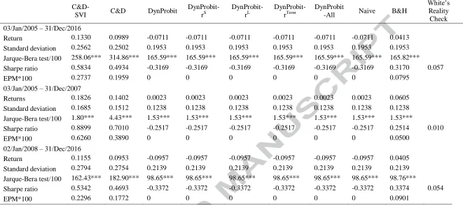
Table 7 presents the results of economic value under the first scenario where
19 due to Lesmond et al. (1999).11 However, our findings are also robust to the different
measures of transaction costs discussed above.12
[Insert Table 7 around here]
During the full out-of-sample period (January 1, 2005 – December 31, 2016), the
passive B&H strategy generates an average return of 4.1%, which combined with a standard
deviation of 19.5% leads to a Sharpe ratio of 0.317. The active strategy based on the
C&D-SVI model clearly outperforms the passive strategy as it yields a Sharpe ratio of 0.324. This
finding, which reflects the good predictive performance of the C&D-SVI model in terms of
sign predictability, is robust across all considered periods and is the result of both higher
average returns and lower volatility.13 In other words, this active strategy will switch from the
stock index into the risk-free asset whenever negative returns are predicted, thus effectively
reducing the downside risk of the portfolio. As a further check, Table 7 presents the results of
the White’s Reality Check procedure which tests the null hypothesis that the best active
strategy in terms of Sharpe ratios is not superior to the B&H strategy. Our findings indicate
that the C&D-SVI, which is the best strategy in our case, overall leads to statistically better
economic gains relative to the passive strategy. Finally, considering the more comprehensive
EPM measure due to Homm and Pigorsch (2012) the relative performance of the active
strategies remain unaffected, thus strengthening the robustness of our findings.14
Turning to the second and less restrictive scenario, where short-sales are allowed, the
corresponding results are tabulated in Table 8. Across all periods, we observe that the best
strategy is still the one associated with the C&D-SVI model followed by the one based on the
C&D model. Interestingly, in this scenario the remaining active strategies not only
underperform the B&H strategy as in the first scenario but they consistently lead to economic
losses. This is congruent with the notion that good predictive performance in statistical terms
(as documented in Section 4.2) does not guarantee economic gains (see, Leitch and Tanner,
1991). Overall, the results based on these alternative models under both scenarios are broadly
in contrast to recent evidence by Nyberg (2011) and Chevapatrakul (2013) who report
11
We round up the transaction costs to 3 bps and hence we employ a slightly more conservative value of one-way transaction costs. This means that each round-trip (selling/buying the bond and buying/selling the stock) costs 6 bps.
12
The transaction costs employed in our paper are generally in agreement with those reported in a number of previous studies (e.g., Gencay, 1998; Bajgrowicz and Scaillet, 2012).
13
To give a better picture of when any positive profit from this strategy would be eliminated, we also estimate its break-even transaction costs. Specifically, we find that these costs are 6.2 bps and 8.5 bps, respectively, for the first and second scenario considered in our study.
14
20 economic gains, albeit without allowing for short-sales. A plausible explanation for this
finding could be the use of higher frequency data in our study which are associated with
lower expected returns and potentially higher number of trades that accumulate greater
transaction costs. Moreover, as in the first scenario (i.e. where short-sales are not allowed),
the White’s Reality Check suggests that the strategy based on the C&D-SVI model is
significantly better than the B&H strategy in terms of Sharpe ratios. Finally, we note that our
results remain robust when we employ the EPM measure.
Overall, our paper is the first study to confirm the usefulness of the C&D model for
real-time investors and to also suggest a new variable, ΔSVI, that further enhances its
performance. This is demonstrated by considering different realistic scenarios and various
performance measures. These results are generally in line with the statistical results presented
in the previous sections and further establish the usefulness of the ΔSVI variable in return
sign predictability. Our findings complement the studies by Christoffersen and Diebold
(2006) and Christoffersen et al. (2007) given the lack of empirical evidence regarding the
economic efficacy of their suggested model, which is of particular interest to market
participants.
5. Conclusion
In this paper we empirically investigate whether a measure for information demand, can lead
to better sign forecasts of stock returns. This is of particular interest given that US stock
returns have been proven difficult to predict in the levels. Specifically, we augment a number
of competing GARCH family models with a measure of information demand (approximated
by SVI from Google) and construct one-step-ahead volatility forecasts, which we use within
the Christoffersen and Diebold (2006) framework to predict the sign of stock returns. We
then focus on the economic significance of sign predictability and formulate appropriate
trading strategies from the perspective of a real-time investor. This is a very important
dimension of our study given the lack of empirical evidence within this framework and the
fact that improved sign predictability in a statistical sense does not necessarily mean higher
economic value for investors. In particular, we adopt the approach by Granger and Pesaran
(2000) and consider an investor whose goal is to maximize her utility function using a
time-varying optimal rule which translates sign probability forecasts into investment decisions.
Our empirical application relies on daily data from the S&P 500 index and covers the period
21 Turning to our results, we show that extending all considered GARCH family models
with the change in demand for information variable (ΔSVI) leads to more accurate return
volatility forecasts. We find that this improvement in forecasting power is statistically
significant and robust across different sample periods (including the recent financial crisis).
This result is in line with a small body of relevant work and highlights the usefulness of the
ΔSVI in predicting the volatility of returns during both normal and turbulent periods in the
stock market.
Moreover, when we employ the forecasted volatilities to predict the sign of daily
stock returns we find that the model suggested by Christoffersen and Diebold (2006)
extended with the ΔSVI variable exhibits the best performance among all considered models.
Specifically, it outperforms all types of models either in their standard form or extended with
a number of variables motivated by previous studies on asset pricing and asset return sign
forecasts. This finding holds across all considered periods and is further confirmed by means
of the Diebold and Mariano (1995) statistic.
Finally, we find that there is consistency between the statistical results and the results
of economic value and show that the model of Christoffersen and Diebold (2006) extended
with the ΔSVI variable offers the highest gains for investors. This confirms its usefulness in
the context of return sign predictability. These novel findings hold when we consider
different utility functions, levels of risk aversion and estimates of transaction costs. Our
findings are also robust to different realistic scenarios (with or without short-sales) and
measures of economic value, giving further support to the main conclusions of the paper.
Appendix
The Google Trends database provides data from January 2004 onwards at weekly frequency.
However, if the requested period is up to a quarter, the data is available at daily frequency.
There is a caveat that comes with this, though, due to the way SVI is calculated. Specifically,
the provided index is always scaled to the highest value within the specified sample. This
means that if one obtains daily SVI data for a time period spanning more than a quarter by
downloading data one quarter at a time, such data are not comparable and a time-series of
SVI cannot be constructed in a consistent manner. Others in the literature (e.g., Da et al.,
2015) have addressed this issue by calculating changes (and losing one observation at the
22 adopt an alternative approach to construct a daily time-series of SVI in a consistent manner.
This approach exploits a feature of Google Trends that allows the user to compare SVI for the
same term between different time periods. The important property of this feature is that, in
order to allow for the comparison, all different subsamples are scaled to the single highest
value found among them. Therefore, if one compares between two different quarters, the data
Google Trends provides will be daily and under the same scaling. Therefore, it becomes an
issue of identifying the quarter that contains the day with the highest SVI (through repeated
downloads) and then downloading all other quarters in comparison to that one. This allows
the construction of a series that is properly scaled at the levels, which preserves all the
information contained in the variable, with the added bonus of not losing any observations
within the sample.
The algorithm detailing the steps required for constructing a consistent time-series of SVI
using Google Trends is as follows. Taking advantage of the fact that Google Trends allows
the simultaneous comparison of up to five different time periods at the same time:
1. Download the first five quarters in the sample.
2. Find the quarter that contains the value of 100. Name this quarter .
3. Download together with four other quarters each time until you have downloaded
all quarters contained in the time period of interest.
4. If you reach the final quarter in the period of interest and , then proceed to
step 6.
5. If during any stage in the execution of step 3 , then this means that one of
the other quarters that were downloaded together with now contains 100. The
quarter that contains 100 now becomes the new . Repeat steps 3 and 4.
6. Join all downloaded quarters together in one vector, in chronological order, to obtain
23
References
Amihud, Y., Hurvich, C.M., 2004. Predictive regressions: A reduced-bias estimation method. Journal of Financial and Quantitative Analysis 39(4), 813–841.
Anand, A., Irvine, P., Puckett, A., Venkataraman, K., 2012. Performance of institutional trading desks: An analysis of persistence of trading costs. Review of Financial Studies 25, 557–598.
Andrei, D., Hasler, M., 2014. Investor attention and stock market volatility. Review of Financial Studies, forthcoming.
Andriosopoulos, D., Chronopoulos, D.K., Papadimitriou, F.I., 2014. Can the information content of share repurchases improve the accuracy of equity premium predictions? Journal of Empirical Finance 26, 96–111.
Aumann, R.J., Seranno, R., 2008. An economic index of riskiness. Journal of Political Economy 116, 810–836.
Awartani, B.M.A., Corradi, V., 2005. Predicting the volatility of the S&P 500 stock index via GARCH models: The role of asymmetries. International Journal of Forecasting 21, 167–183.
Bekiros, S.D., 2010. Heterogeneous trading strategies with adaptive fuzzy Actor-Critic reinforcement learning: A behavioural approach. Journal of Economic Dynamics and Control 34, 1153–1170.
Bhardwaj, R.K., Brooks, L.D., 1992. The January anomaly: Effects of low share price, transaction costs, and bid-ask bias. Journal of Finance 47, 553–574.
Bollerslev, T., 1986.Generalised autoregressive heteroscedasticity. Journal of Econometrics 31, 307–327.
Bossaerts, P., Hillion, P., 1999. Implementing statistical criteria to select return forecasting models: What do we learn? Review of Financial Studies, 12(2), 405−428.
Boudoukh, J., Michaely, R., Richardson, M., Roberts, M.R., 2007. On the importance of measuring payout yield: Implications for empirical asset pricing. Journal of Finance, 62(2), 877–915.
Brier, G.W., 1950. Verification of forecasts expressed in terms of probabilities. Monthly Weather Review 78, 1−3.
Brooks, C., 1998. Predicting stock index volatility: Can market volume help? Journal of Forecasting 17(1), 59–80.
Campbell, J.Y., Shiller, R.J., 1988. The dividend-price ratio and expectations of future dividends and discount factors. Review of Financial Studies 1(3), 195−228.
Campbell, J.Y., Thompson, S.B., 2008. Predicting excess stock returns out of sample: Can anything beat the historical average? Review of Financial Studies 21(4), 1509−1531. Chevapatrakul, T., 2013. Return sign forecasts based on conditional risk: Evidence from the
UK stock market index. Journal of Banking and Finance 37, 2342−2353.
Christoffersen, P.F., Diebold, F.X., 2006. Financial asset returns, direction-of-change forecasting, and volatility dynamics. Management Science 52(8), 1273–1287.
Christoffersen, P.F., Diebold, F.X., Mariano, R., Tay, A., Tse, Y., 2007. Direction-of-change forecasts based on conditional variance, skewness and kurtosis dynamics: International Evidence. Journal of Financial Forecasting 1, 3–24.
Da, Z., Engelberg, J., Gao, P., 2011. In search of attention. Journal of Finance 66, 1461– 1499.
24 Della Corte, P. Sarno, L., Valente, G., 2010. A century of equity premium predictability and the consumption-wealth ratio: An international perspective. Journal of Empirical Finance 17, 313–331.
Diebold, F.X., Lopez, J.A., 1996. Forecast evaluation and combination. NBER Working Paper No. 192.
Diebold, F.X., Mariano, R.S., 1995. Comparing predictive accuracy. Journal of Business and Economics Statistics 13, 253–263.
Dimpfl, T., Jank, S., 2015. Can internet search queries help to predict stock market volatility? European Financial Management, forthcoming.
Fama, E.F., French, K.R., 1988. Dividend yields and expected stock returns. Journal of Financial Economics 22(1), 3−25.
Fama, E.F., Blume, M.E., 1966. Filter rules and stock market trading. Journal of Business 39, 226−241.
Ferson, W.E., Sarkissian, S., Simin, T.T., 2003. Spurious regressions in financial economics? Journal of Finance 58(4), 1393–1413.
Gerlach, J.R., 2005. Imperfect information and stock market volatility. Financial Review 40, 173–194.
Glosten, L.R., Jagannathan, R., Runkle, D.E., 1993. On the relation between the expected value and the volatility of the nominal excess returns on stocks. Journal of Finance 48(5) 1779–1801.
Goddard, J., Kita, A., Wang, Q., 2015. Investor attention and FX market volatility. Journal of International Financial Markets, Institutions, and Money 38, 79–96.
Goetzmann, W. N., Jorion, P., 1993.Testing the predictive power of dividend yields. Journal of Finance 48(2), 663–679.
Goetzmann, W.N., Ingersoll, J., Spiegel, M., Welch, I., 2007. Portfolio performance manipulation and manipulation-proof performance measures. Review of Financial Studies 20, 1503–1546.
Golec, J., Tamarkin, M., 1998. Bettors love skewness, not risk, at the horse track. Journal of Political Economy 106, 205–225.
Goyal, A., Welch, I., 2003.Predicting the equity premium with dividend ratios. Management Science 49(5), 639–654.
Goyal, A., Welch, I., 2008.A comprehensive look at the empirical performance of equity premium prediction. Review of Financial Studies 21(4), 1455–1508.
Granger, C.W.J., Pesaran, M.H., 2000.Economic and statistical measures of forecast accuracy. Journal of Forecasting 19(7), 537–560.
Harvey, C.R., Sidique, A., 2000. Conditional skewness in asset pricing tests. Journal of Finance 55, 1263–1295.
Hodrick, R.J., 1992. Dividend yields and expected stock returns: Alternative procedures for inference and measurement. Review of Financial Studies 5(3), 357−386.
Homm, U., Pigorsch, C., 2012. Beyond the Sharpe ratio: An application of the Aumann-Seranno index to performance measurement. Journal of Banking and Finance 36, 2274–2284.
Hsieh, D.A., 1991. Chaos and nonlinear dynamics: Application to financial markets. Journal of Finance 46(5), 1839–1877.
Hsu, P.H., Kuan, C.M., 2005. Re-examining the profitability of technical analysis with data snooping checks. Journal of Financial Econometrics 3, 606–628.
Inoue, A., Kilian, L., 2004. In-sample or out-of-sample tests of predictability: Which one should we use? Econom. Rev. 23, 371–402.
25 Jordan, S.J., Vivian, A.J., Wohar, M.E., 2014. Forecasting returns: New European evidence.
Journal of Empirical Finance 26, 76–95.
Kostakis, A., Magdalinos, T., Stamatogiannis, M.P., 2015. Robust econometric inference for stock return predictability. Review of Financial Studies, forthcoming.
Kellard, N.M., Nankervis, J.C., Papadimitriou, F.I., 2010. Predicting the equity premium with dividend ratios: Reconciling the evidence. Journal of Empirical Finance 17(4), 539– 551.
Lamont, O., 1998. Earnings and expected returns. Journal of Finance 53(5), 1563–1587. Leitch, G., Tanner, J.E., 1991. Econometric forecast evaluation: Profits versus the
conventional error measures. American Economic Review 81, 580–590.
Lesmond D.A., Ogden, J.P., Trzcinka, C.A., 1999. A new estimate of transaction costs. Review of Financial Studies 12(5), 1113–1141.
Lettau, M., Ludvigson, S., 2001. Consumption, aggregate wealth and expected stock returns. Journal of Finance 56(3), 815–849.
Lewellen, J., 2004. Predicting returns with financial ratios. Journal of Financial Economics 74(2), 209−235.
Li, G., 2005. Information quality, learning, and stock market returns. Journal of Financial and Quantitative Analysis 40, 595–620.
Maio, P., 2013. The “Fed model” and the predictability of stock returns. Review of Finance 17, 1489–1533.
McCracken, M.W., 2007.Asymptotics for out-of-sample tests of Granger causality. Journal of Econometrics 140, 719–752.
Moscarini, G., Smith, L., 2002. The law of large demand for information. Econometrica 70, 2351–2366.
Nelson, D.B., 1991. Conditional heteroscedasticity in asset returns: A new approach. Econometrica 59(2), 347–370.
Nelson, C.R., Kim, M.J., 1993. Predictable stock returns: the role of small sample bias. Journal of Finance 48(2), 641–661.
Nyberg, H., 2011. Forecasting the direction of the US stock market with dynamic binary probit models. International Journal of Forecasting 27, 561–578.
Pagan, A.R., Schwert, G.W., 1990.Alternative models for conditional stock volatility. Journal of Econometrics 45(1-2), 267–290.
Pesaran, M.H., Timmermann, A., 2000. A recursive modelling approach to predicting UK stock returns. Economic Journal 110, 159−191.
Pontiff, J., Schall, L.D., 1998.Book-to-market ratios as predictors of market returns. Journal of Financial Economics 49(2), 141−160.
Poon, S.H., Granger, C.W.J., 2003. Forecasting volatility in financial markets: A review. Journal of Economic Literature 41, 478−539.
Poon, S.H., Granger, C.W.J., 2005. Practical issues in forecasting probability. Financial Analysts Journal 61(1), 45−56.
Rapach, D.E., Zhou, G., 2013. Forecasting stock returns. In Graham Elliott and Allan Timmermann, eds: Handbook of Economic Forecasting, Volume 2 (Elsevier, Amsterdam).
Ross, S.A., 1989. Information and volatility: The no-arbitrage martingale approach to timing and resolution irrelevancy. Journal of Finance 44, 1–17.
Rozeff, M., 1984. Dividend yields are equity risk premiums. Journal of Portfolio Management 11(1), 68−75.
26 Stoll, H.R., Whaley, R., 1983. Transaction costs and the small firm effect. Journal of
Financial Economics 12, 57–79.
Taylor, S., 1986. Modelling Financial Time Series. Wiley, Chichester.
Vlastakis, N., Markellos, R.N., 2012. Information demand and stock market volatility. Journal of Banking & Finance 36(6), 1808–1821.
Vozlyublennaia, N., 2014. Investor attention, index performance, and return predictability. Journal of Banking & Finance 41, 17–35.
West, K.D., 1996. Asymptotic inference about predictive ability. Econometrica 64, 1067– 1084.
27
[image:29.595.112.482.191.475.2]FIGURES
Figure 1. Time series graph of the information demand variable (SVI)