June 2, 2014
The protoplanetary disk of FT Tauri:
multi-wavelength data analysis and modeling
?
A. Garufi
1, L. Podio
2,3, I. Kamp
4, F. M´enard
2,5, S. Brittain
6, C. Eiroa
7, B. Montesinos
8,
M. Alonso-Mart´ınez
7, W.F. Thi
2, and P. Woitke
9,10,111 Institute for Astronomy, ETH Z¨urich, Wolfgang-Pauli-Strasse 27, CH-8093 Zurich, Switzerland
e-mail:[email protected]
2 CNRS/UJF Grenoble 1, UMR 5274, Institut de Plan´etologie et d’Astrophysique de Grenoble (IPAG), France 3 INAF - Osservatorio Astrofisico di Arcetri, Largo E. Fermi 5, 50125, Florence, Italy
4 Kapteyn Astronomical Institute, Postbus 800, 9700 AV Groningen, The Netherlands
5 UMI-FCA, CNRS/INSU, France (UMI 3386), and Dept. de Astronom´ıa, Universidad de Chile, Santiago, Chile 6 Department of Physics & Astronomy, 118 Kinard Laboratory, Clemson University, Clemson, SC 29634, USA 7 Dpt. F´ısica Te´orica, Facultad de Ciencias, Universidad Aut´onoma de Madrid, Cantoblanco, 28049 Madrid, Spain
8 Dpt. de Astrof´ısica, Centro de Astrobiolog´ıa, ESAC Campus, P.O. Box 78, E-28691 Villanueva de la Ca˜nada, Madrid, Spain 9 University of Vienna, Dept. of Astronomy, Turkenschanzstr. 17, A-1180 Vienna, Austria
10 UK Astronomy Technology Centre, Royal Observatory, Edinburgh, Blackford Hill, Edinburgh EH9 3HJ, UK 11 SUPA, School of Physics & Astronomy, University of St. Andrews, North Haugh, St. Andrews KY16 9SS, UK
Received ....; accepted ....
ABSTRACT
Context.Investigating the evolution of protoplanetary disks is crucial for our understanding of star and planet formation. Several theoretical and observational studies have been performed in the last decades to advance this knowledge. The launch of satellites operating at infrared wavelengths, such as theSpitzerSpace Telescope and theHerschelSpace Observatory, has provided important tools for the investigation of the properties of circumstellar disks.
Aims.FT Tauri is a young star in the Taurus star forming region that was included in a number of spectroscopic and photometric surveys. We investigate the properties of the star, the circumstellar disk, and the accretion/ejection processes and propose a consistent gas and dust model also as a reference for future observational studies.
Methods. We performed a multi-wavelength data analysis to derive the basic stellar and disk properties, as well as mass accre-tion/outflow rate from TNG/DOLoRes, WHT/LIRIS, NOT/NOTCam, Keck/NIRSpec, andHerschel/PACS spectra. From the liter-ature, we compiled a complete Spectral Energy Distribution. We then performed detailed disk modeling using theMCFOST and ProDiMocodes. Multi-wavelength spectroscopic and photometric measurements were compared with the reddened predictions of the codes in order to constrain the disk properties.
Results.We determine the stellar mass (∼0.3 M), luminosity (∼0.35 L) and age (∼1.6 Myr), as well as the visual extinction of
the system (1.8 mag). We estimate the mass accretion rate (∼3·10−8M/yr) to be within the range of accreting objects in Taurus. The evolutionary state and the geometric properties of the disk are also constrained. The radial extent (0.05 to 200 AU), flaring angle (power-law with exponent=1.15), and mass (0.02 M) of the circumstellar disk are typical of a young primordial disk. This object
can serve as a benchmark for primordial disks with significant mass accretion rate, high gas content and typical size.
Key words.stars: pre-main sequence – planetary systems: protoplanetary disks – accretion, accretion disks – ISM: individual object: FT Tau
1. Introduction
Protoplanetary disks are the birthplaces of planets and the study of their physical and chemical structure can help us understand planet formation. By studying a large sample of young proto-planetary disks (class II) in detail, we may be able to assess the variety in disk structure and to match that to the ever growing diversity in exoplanetary systems architecture.
The disk evolution can be observationally constrained by studying the Spectral Energy Distribution (SED) of Young Stellar Objects (YSOs) in different evolutionary stages. In par-ticular, the mass accretion rate can be estimated from the excess in the UV and optical spectra and from emission lines that are
?
Based onHerscheldata.Herschelis an ESA space observatory with science instruments provided by European-led Principal Investigator consortia and with important participation from NASA.
thought to form in the magnetospheric accretion process (Basri & Bertout 1989, Edwards et al. 1994, Hartmann, Hewett, & Calvet 1994).
Also geometrical properties of circumstellar disks change with time. In the absence of spatially resolved images, the ge-ometry has to be constrained from infrared (IR) and millimetric photometry. A flaring geometry is a natural explanation for the strong far-infrared (FIR) flux shown by most sources (Kenyon & Hartmann 1987). Grain-grain collisions result in dust grain growth and, on timescales of 104−106years, grains are thought
to settle to the mid-plane leaving the gas at the disk surface ex-posed to direct stellar radiation (Bouwman et al. 2008). This evo-lution is reflected in decreasing mid-infrared (MIR) fluxes and in a widening and flattening of the 10µm and 18µm silicate fea-tures (e.g. Furlan et al. 2006, Fang et al. 2009).
The diagnostic of gas emission lines from the disk is another pivotal tool for the study of the disk structure. CO and OH lines are commonly detected in the near-infrared (NIR) spectra of pro-toplanetary disks. In particular, the CO fundamental (ν=1−0) lines in the M band are excellent tracers of the temperature and density structure inside a few AU, the terrestrial planet-forming regions, because of their sensitivity to low column densities of gas at temperatures of a few 1000 K (Najita et al. 2000). On the other hand, the frequently observed FIR [Oi] 63µm line (Dent et al. 2013) is believed to mostly originate in the colder outer regions, between 30 and 100 AU (Kamp et al. 2010). Its flux can be used in combination with other lines as an indicator of disk gas mass.
An ever growing number of datasets is becoming available for circumstellar disks. Nevertheless, many studies still focus on the interpretation of a single dataset even in the framework of detailed disk modeling. However, full characterization of stellar and circumstellar properties of single objects is often reached only by employing dust and gas diagnostic measurements (pho-tometry and line emission) that cover the entire extent of a pro-toplanetary disk. In this paper, we aim to investigate the geo-metrical and chemical properties of the disk around the T Tauri Star (TTS) FT Tauri, by means of a multi-wavelength dataset and consistent dust and gas modeling.
Even though the Taurus star forming region and its members are well studied (e.g. Kenyon et al. 1994, Gullbring et al. 1998, Luhman et al. 2010, Rebull et al. 2010), a comprehensive char-acterization has been restricted so far to either extremely bright (large) disks (e.g. DM Tau, Guilloteau & Dutrey 1994) or ex-ceptional objects (e.g. LkCa15, van Zadelhoffet al. 2001). FT Tau is located in the South of the Barnard 215 dark cloud and is surrounded by extended emission (see Sloan Digital Sky Survey optical image from Finkbeiner et al. 2004). This source is far from most of the known Taurus members (see extinction map of Taurus from Dobashi et al. 2005). No X-ray emission was de-tected at the optical position of the star (Neuh¨auser et al. 1995). FT Tau was included in a number of photometric and spectro-scopic surveys at different wavelengths. The main stellar and disk properties from the literature are shown in Table 1. With more sensitive interferometers such as SMA and IRAM/PdBI, FT Tau can serve as an excellent target for more detailed astro-chemical studies.
The multi-wavelength data used in this work and its data re-duction is presented in Sect. 2 and a detailed analysis thereof in Sect. 3. The result of this analysis are then further used in Sect. 4 to build consistent dust and gas models (MCFOST and
ProDiMo) for FT Tau. Sect. 5 then discusses the results and the
source variability.
2. Observations and data reduction
The data analysed in this paper consist of spectroscopy at opti-cal, NIR, and FIR wavelengths from the Telescopio Nazionale Galileo (TNG), the William Herschel Telescope (WHT), the Nordic Optical Telescope (NOT), the Keck Observatory, and the
HerschelSpace Observatory. The instrumental settings for the
spectroscopic observations are presented in detail in the follow-ing sections and summarized in Table 2. Additional data were retrieved from the literature and consist of MIR spectroscopy
fromSpitzerSpace Telescope and of photometry from optical to
radio wavelengths (see Table 3 and Fig. 1).
Table 1.Properties of FT Tauri estimated in previous works.
Coordinates (J2000):
Right ascension α 04h23m39s.19 a Declination δ +24◦
560
1400
.11 a Proper motion:
Right ascension µα +6.3±3.3 mas yr−1 b
Declination µδ -15.3±3.3 mas yr−1 b Stellar properties:
Visual extinction AV 3.8 c
Spectral type M3e c
Luminosity L∗ 0.63 L c
Disk properties:
Gas mass Md 0.05±0.03 M d
Outer radius Rout 50+−95025 AU d
a Cutri et al. 2003; b Luhman et al. 2009; c Rebull et al. 2010; d
Andrews & Williams 2007.
2.1. TNG/DOLORES observations
We present spectroscopic data of FT Tau obtained using the DOLORES spectrograph, the Device Optimized for the LOw RESolution (Oliva 2004) mounted on the TNG (La Palma Observatory). The observations were performed in November 2009 with the VHR-V grism (λ/∆λ = 1527 for a slit width of 1”), covering the wavelength range from 4752 Å to 6698 Å.
Three observations (exposure times of 1400, 600, and 200 s) were performed in seeing-limited conditions (FWHM'1.25”). The DOLORES spectra were reduced using the IRAF software package. The 2-D spectra were flat-fielded, sky-subtracted and wavelength calibrated using the Argon arc lamp. Then, the 1-D spectrum was extracted by integrating over the source spatial profile and corrected for telluric absorption features. No photo-metric standard observations were taken. Thus, the flux calibra-tion was obtained from previous photometry in the V band (see Table 3). Figure 1a shows that the V band photometry agrees well with the neighboring SDSS photometry. This approach is not taking into account the source variability, which is further discussed in Sect. 5.1.
2.2. WHT/LIRIS observations
A J-band (1.18 - 1.40 µm) spectrum was taken in December 2009 with the LIRIS, Long-slit Intermediate Resolution Infrared Spectrograph, at the WHT (La Palma Observatory). The spec-trum was acquired with a 0.7500slit width and the LIRIS hrj grism
providing a spectral resolution ofλ/∆λ = 2200. The exposure time was 120 seconds. The data reduction was carried out using IRAF. After flat-field correction and sky subtraction, an Argon lamp was used for wavelength calibration of the 1-D extracted spectrum. The flux calibration was performed by means of the 2MASS photometry (see Table 3 and Fig. 1b).
2.3. NOT/NOTCAM observations
A K-band spectrum of FT Tau was taken with the NOTCAM, the Nordic Optical Telescope CAMera (Aspin 1999) of the NOT (La Palma Observatory). These observations were acquired in December 2009 by using the K grism (λ/∆λ = 1500 for a slit width of 1”), operating in the NIR K-band (1.95 - 2.37µm), and nodding the slit between two positions.
Table 2.Instrumental settings for the spectroscopic observations of FT Tau.
Observation date Instrument Slit width (”) Spectral range (µm) Spectral resolution (km/s) Integration time (s)
2009-11-26 TNG/DOLORES 1 0.475 - 0.670 196 1400, 600, 200
2009-12-04 NOT/NOTCAM 1 1.95 - 2.37 200 48
2009-12-09 WHT/LIRIS 0.75 1.17 - 1.35 135 120
2008-12-10 Keck/NIRSPEC 0.43 4.42 - 5.53 12 960, 1200
2010-03-26 Herschel/PACS Integral field 62.95 - 63.40 88 1152
The observation was obtained in seeing-limited conditions (FWHM'0.9”) with an exposure time of 48 s. The data reduc-tion of the spectrum was performed using the IRAF software. The spectrum was background-subtracted and flat-fielded. The 1-D spectrum was extracted and wavelength calibrated through Argon arc lamp. Since no photometric standard observations were available, the flux calibration of these data was performed exploiting the KS photometry from 2MASS (see Table 3 and
Fig. 1c).
2.4. Keck/NIRSPEC observations
An M-band high-resolution spectrum of FT Tau was taken with the NIRSPEC, the NIR SPECtrograph (McLean et al. 1998) on the W.M. Keck Observatory. The spectra were obtained in December 2008 using the M-Wide filter and 0.43” slit providing a resolution of λ/∆λ = 25,000. The spectra span 4.67 - 5.05 µm. FT Tau was observed for 16 and 20 minutes in successive exposures.
Because of the thermal background in the M-band, the data were observed in an ABBA sequence where the telescope was nodded 12” between the A and B positions. Each frame was flat fielded and scrubbed for hot pixels and cosmic ray hits. The ob-servations were combined as (A-B-B+A)/2 in order to cancel the sky emission. The data were rectified in the spatial direc-tion by fitting a polynomial to the point spread funcdirec-tion (PSF) of the star in each column. The data were rectified in the spec-tral direction by fitting a sky emission model generated by the Spectral Synthesis Program (Kunde & Maguire 1974) to each row and interpolating the wavelength solution to each row to the row in the middle of the detector.
Regions in which the transmittance was less than 50% were masked. The wavelength calibration was determined from the fit to the telluric absorption lines and is generally accurate to within about 0.1 pixels (∼0.4 km/s). Flux calibration was performed us-ing the available Spitzer/IRAC 4.5 and 5.8µm photometry (see Table 3 and Fig. 1d). In order to obtain the gas velocity with re-spect to the star, we corrected for the observed radial velocity of FT Tau, as estimated by Guilloteau et al. (2013) (vLSR =7−9
km/s).
2.5. Herschel/PACS observations
FIR spectroscopic observations of FT Tau were obtained with the integral-field spectrometer PACS (Poglitsch et al. 2010), on board of the Herschel Space Telescope (Pilbratt et al. 2010) as part of theHerschelOpen Time Key Project GASPS (GAS in Protoplanetary Systems, PI: W. Dent, see Dent et al. 2013). The observations were carried out in the chop- nod mode to re-move the background emission and with a single pointing on the source. They cover simultaneously a selected wavelength range in the blue and in the red arms. In particular, the
obser-vation acquired in line mode (OBSID: 1342192790) covers the ranges 63.0–63.4µm and 180.7–190.3µm, with a resolution of 88 km s−1 and 200 km s−1. The observation acquired in range
mode (OBSID: 1342243501) covers the ranges 71.8–73.3 µm and 143.5–146.6 µm, with a spectral resolution of 162 km s−1 and 258 km s−1.
Data were reduced using HIPE 10. Removal of saturated and bad pixels, chop subtraction, flat-field correction, and mean of two nods were performed by means of the available PACS pipeline.
Photometric FIR observations of FT Tau were also taken
with Herschel/PACS within the GASPS project. The obtained
photometric measurements at 70, 100, and 160µm are presented in Howard et al. (2013) and shown in Table 3.
2.6. Photometric and Spitzer/IRS observations
We collected from the literature 44 photometric measurements of FT Tau, from 0.36 µm to 7 mm (see Table 3 for the fluxes and references). These data have been acquired with 14 different instruments and over more than two decades (see Sect. 5.1 and Appendix A for a further discussion on variability).
A MIR spectrum of FT Tau (spectral range 5.13µm - 39.90 µm) was also retrieved from the literature (Furlan et al. 2006).
3. Results from observations
The spectra obtained by reducing the observations presented in Sect. 2 are shown in Fig. 1. The optical TNG spectrum (Fig. 1a) shows a number of molecular absorption bands, that are typical of late-type stars, and several emission lines, which are thought to originate from the accretion columns or from the outflow. The J-band WHT spectrum (Fig. 1b) and the K-band NOT spectrum (Fig. 1c) show prominent Paβand Brγemission lines, produced in the accretion process. In the Keck spectra (Fig. 1d, 1d1, 1d2) we detected the Pfβand Hu recombination lines, and CO ro-vibrational lines which are thought to be produced in the disk by thermal excitation or by UV fluorescence. The spectroscopic ob-servations collected withHerschel/PACS cover a number of disk tracers, e.g. water lines (o-H2O 707-616, p-H2O 413-322), high-J
rotational CO lines (CO J=18-17, and CO J=36-35), the CH+ J=5-4, and the [Oi] 3P1-3P2 and [Oi] 3P0-3P1 lines at 63.184
0.5 0.55 0.6 0.65
Wavelength (μm)
1x10-11 1x10⁻¹⁰ 1x10⁻⁹
λ
·
F (λ) (erg
·
s⁻¹
·
cm⁻²)
Hβ FeII FeII HeI NaD [OI] Hα HeI
(a)
1.18 1.2 1.22 1.24 1.26 1.28 1.3 1.32 1.34
Wavelength (μm)
3x10⁻¹⁰
4x10⁻¹⁰
5x10⁻¹⁰
6x10⁻¹⁰
7x10⁻¹⁰ 8x10⁻¹⁰
9x10⁻¹⁰
λ
·
F (λ) (erg
·
s⁻¹
·
cm⁻²)
Paβ (b)
2.05 2.1 2.15 2.2 2.25 2.3 2.35
Wavelength (μm)
3x10⁻¹⁰
3.5x10⁻¹⁰
4x10⁻¹⁰
4.5x10⁻¹⁰
λ
·
F (λ) (erg
·
s⁻¹
·
cm⁻²)
Brγ
(c)
4.66 4.7 4.74 4.78 4.96 5.0 5.04 5.08 Wavelength (μm)
6x10-11
1x10⁻¹⁰
1.4x10⁻¹⁰
1.8x10⁻¹⁰
2.2x10⁻¹⁰
λ
·
F (λ) (erg
·
s⁻¹
·
cm⁻²)
Pfβ Huε
(d)
5 10 15 20 25 30 35
Wavelength (μm)
1x10⁻¹⁰
λ
·
F (λ) (erg
·
s⁻¹
·
cm⁻²)
Silicate features
(e)
63 63.1 63.2 63.3 63.4
Wavelength (μm)
0 1x10-11 2x10-11 3x10-11 4x10-11 5x10-11
λ
·
F (λ) (erg
·
s⁻¹
·
cm⁻²)
[OI] 63μm
(f)
4.68 4.7 4.72 4.74 4.76 4.78
Wavelength (μm) 5x10-11
1x10⁻¹⁰
1.5x10⁻¹⁰ 2x10⁻¹⁰
λ
·
F (λ) (erg
·
s⁻¹
·
cm⁻²)
1-0 P2
1-0 P1 1-0 P3 1-0 P4 1-0 P5 1-0 P6 1-0 P7 1-0 P8 2-1 P2
1-0 P9 1-0 P10 1-0 P11 2-1 P5
1-0 P12
(d1)
4.96 4.98 5 5.02 5.04 5.06 5.08 5.1
Wavelength (μm)
0 5x10-11
1x10⁻¹⁰
1.5x10⁻¹⁰
2x10⁻¹⁰
λ
·
F (λ) (erg
·
s⁻¹
·
cm⁻²)
1-0 P30 1-0 P32 2-1 R26
1-0 P36 1-0 P37 1-0 P38 1-0 P39 1-0 P40 2-1 R25
1-0 P31
2-1 R27
[image:4.595.106.503.50.734.2](d2)
Fig. 1.Spectroscopic observations. (a) TNG optical spectrum; (b) WHT J-band spectrum; (c) NOT K-band spectrum; (d) Keck high-resolution spectra; (e) Spitzer MIR spectrum; (f)HerschelFIR spectrum of the only detected line ([Oi] 63 µm); (d1) and
(d2) zoom on the CO lines detected in the Keck spectra. Photometric non-simultaneous observations are plotted as color symbols. Spectra shown in (a), (b), (c) were flux-calibrated by means of the photometry.
Table 3.Photometric measurements of FT Tau.
Instrument λ Band Flux λFλ
(µm) (publication units) (erg·cm−2·s−1)
SDSS 0.36 u band 16.681±0.007 mag a (6.69±0.06)·10−12 USNO 0.44 B band 15.48 mag b 1.80·10−11 SDSS 0.48 g band 15.804±0.004 mag a (1.08±0.01)·10−11 USNO 0.55 V band 14.69 mag b 2.64·10−11 SDSS 0.62 r band 14.254±0.004 mag a (3.47±0.02)·10−11 USNO 0.68 R band 12.06 mag b 1.07·10−10 SDSS 0.76 i band 15.023±0.011 mag a (6.39±0.06)·10−11 USNO 0.80 I band 11.36 mag b 2.56·10−10 SDSS 0.90 z band 12.456±0.004 mag a (1.22±0.01)·10−10 2MASS 1.25 J band 10.19±0.03 mag d (3.15±0.07)·10−10 2MASS 1.65 H band 9.12±0.03 mag d (4.58±0.11)·10−10 2MASS 2.16 KSband 8.59±0.02 mag d (3.32±0.06)·10−10 WISE 3.37 7.75±0.02 mag e (2.18±0.04)·10−10 Spitzer/IRAC 3.6 7.64±0.02 mag f (2.06±0.04)·10−10 Spitzer/IRAC 3.6 7.89±0.02 mag f (1.57±0.07)·10−10 Spitzer/IRAC 4.5 7.12±0.02 mag f (1.72±0.03)·10−10 Spitzer/IRAC 4.5 7.44±0.02 mag f (1.24±0.06)·10−10 WISE 4.61 7.10±0.02 mag e (1.60±0.03)·10−10 Spitzer/IRAC 5.8 6.81±0.02 mag f (1.15±0.02)·10−10 Spitzer/IRAC 5.8 7.12±0.02 mag f (7.91±0.36)·10−11 Spitzer/IRAC 8.0 5.95±0.03 mag f (1.00±0.03)·10−10 Spitzer/IRAC 8.0 6.27±0.03 mag f (7.32±0.33)·10−11 IRAS 12 0.46 Jy±14% g (1.15±0.16)·10−10 WISE 12.08 5.09±0.01 mag e (7.23±0.06)·10−11 WISE 22.19 3.08±0.02 mag e (6.59±0.12)·10−11 Spitzer/MIPS 24 3.15±0.04 mag f (4.90±0.17)·10−11 IRAS 25 0.65 Jy±12% g (7.80±0.94)·10−11 IRAS 60 0.86 Jy±10% g (4.30±0.43)·10−11 Spitzer/MIPS 70 0.28±0.22 mag h (2.56±0.47)·10−11 Herschel/PACS 70 0.73±0.07 Jy i (3.08±0.30)·10−11 IRAS 100 1.92 Jy±14% g (5.76±0.81)·10−11 Herschel/PACS 100 0.95±0.09 Jy i (2.76±0.27)·10−11 Herschel/PACS 160 1.27±0.19 Jy i (2.34±0.36)·10−11 CSO 350 1106±82 mJy j (9.48±0.70)·10−12 JCMT 450 437±56 mJy j (2.91±0.37)·10−12 CSO 624 260±100 mJy k (1.25±0.48)·10−12 CSO 769 250±50 mJy k (9.75±1.95)·10−13 JCMT 850 121±5 mJy j (4.27±0.17)·10−13 SMA 880 111±2 mJy l (3.78±0.07)·10−13 CSO 1056 137±40 mJy k (3.89±1.13)·10−13 IRAM 1300 130±14 mJy m (3.00±0.32)·10−13 IRAM 2700 25±2.2 mJy n (2.78±0.24)·10−14 VLA 7000 1.62±0.27 mJy o (6.94±1.15)·10−16
References:aFinkbeiner et al. 2004;bMonet et al. (2003);dCutri et al. (2003);eWright et al. 2010;fLuhman et al. (2010), two observations per wavelength;gBeichman et al. (1988);hRebull et al. (2010);iHoward et al. (2013);jAndrews & Williams (2005);kBeckwith & Sargent (1991); lAndrews & Williams (2007);mBeckwith et al. (1990);nDutrey et al. (1996);oRodmann et al. (2006).
In this section we describe the methods applied to derive the stellar properties (Sect. 3.1), a few disk properties (Sect. 3.2), and the mass accretion and outflow rates (Sect. 3.3).
3.1. Stellar properties
First, we determined the spectral type of FT Tau by comparing the optical TNG spectrum with the spectra of the MILES stel-lar libraries (Sanchez-Blazquez et al. 2006). The observed ab-sorption features suggest that FT Tau is an M2 or M3 star, in agreement with the result by Rebull et al. (2010). The tempera-ture scale is based on Cohen & Kuhi (1979). Then, we adopted
a PHOENIX model (Teff =3400 K, log(g)=3.5, [Fe/H]=0.0)
of the stellar atmosphere (Hauschildt et al. 1999) to reproduce the stellar spectrum of the source.
Table 4.Emission lines detected in our spectra and respective vacuum wavelengths. When the line presents instrumental gaps, lower and higher estimates due to the missing region are included in the error. Dereddened fluxes are omitted when the correction for the extinction is negligible.
Line Wavelength Instrument Observed flux Dereddened flux (AV =1.8) Likely origin (µm) (10−14erg·s−1·cm−2) (10−14erg·s−1·cm−2)
Hβ 0.486 TNG 17.9±0.3 125.5 Accretion
Feii 0.492 TNG 0.73±0.03 4.9 Accretion
Feii 0.502 TNG 0.83±0.03 5.6 Accretion
Feii 0.517 TNG 1.65±0.07 7.1 Accretion
Hei 0.588 TNG 2.63±0.31 12.1 Accretion
NaD 0.589 TNG 0.62±0.03 4.8 Accretion
NaD 0.590 TNG 0.34±0.03 2.7 Accretion
[Oi] 0.630 TNG 0.68±0.21 2.6 Disk/Outflow
Hα 0.654 TNG 169.4±0.6 679.8 Accretion
Hei 0.668 TNG 1.69±0.05 6.9 Accretion
Paβ 1.282 WHT 30.5±0.7 46.0 Accretion
Brγ 2.166 NOT 12.5±0.8 14.6 Accretion
Pfβ 4.654 Keck 4.45±0.21 - Accretion
CO 1−0 P1 4.674 Keck 0.30±0.11 - Disk
CO 1−0 P2 4.683 Keck 1.16+0.13
−0.28 - Disk
CO 1−0 P3 4.691 Keck 1.39+0.17
−0.51 - Disk
CO 1−0 P4 4.699 Keck 1.65+0.18
−0.38 - Disk
CO 1−0 P5 4.709 Keck 1.25+0.23
−0.28 - Disk
CO 1−0 P6 4.718 Keck 1.48+0.17
−0.22 - Disk
CO 1−0 P7 4.727 Keck 1.97+0.14
−0.18 - Disk
CO 1−0 P8 4.736 Keck 0.90+0.08
−0.10 - Disk
CO 2−1 P2 4.741 Keck 0.26±0.13 - Disk
CO 1−0 P9 4.745 Keck 1.50+0.51
−0.71 - Disk
CO 1−0 P10 4.756 Keck 1.58±0.12 - Disk
CO 2−1 P4 4.759 Keck 0.28±0.10 - Disk
CO 1−0 P11 4.764 Keck 0.66±0.13 - Disk
CO 2−1 P5 4.768 Keck 0.49±0.07 - Disk
CO 1−0 P12 4.774 Keck 1.62+0.12
−0.24 - Disk
CO 1−0 P30 4.967 Keck 1.01±0.19 - Disk
CO 2−1 R25 4.971 Keck 0.41±0.14 - Disk
CO 1−0 P31 4.979 Keck 1.01±0.26 - Disk
CO 1−0 P32 4.991 Keck 0.91±0.21 - Disk
CO 2−1 R27 4.995 Keck 0.25±0.10 - Disk
CO 1−0 P36 5.041 Keck 0.83±0.08 - Disk
CO 2−1 P30 5.043 Keck 0.20±0.07 - Disk
CO 1−0 P37 5.053 Keck 0.61±0.13 - Disk
CO 1−0 P38 5.066 Keck 0.71±0.14 - Disk
CO 1−0 P39 5.079 Keck 0.88±0.18 - Disk
CO 1−0 P40 5.092 Keck 0.86±0.09 - Disk
[Oi] 63.185 Herschel 1.6±0.5 - Disk/Outflow
o−H2O 71.947 Herschel <1.41 -
-CH+5−4 72.140 Herschel <1.37 -
-CO 36−35 72.843 Herschel <0.97 -
-p−H2O 144.518 Herschel <0.32 -
-CO 18−17 144.784 Herschel <0.33 -
-[Oi] 145.525 Herschel <0.31 -
-an extinction ofAV =1.8. For a discussion on the uncertainties affecting the determination of the extinction, see Appendix A.
To determine the stellar luminosity and radius we imposed the reddened PHOENIX flux at 1.25µm to be equal to the ob-served one, as available from 2MASS (see Table 3), assuming that the latter is only due to photospheric emission.
The estimated radius isR∗=1.7 Rand the luminosityL∗=
0.35 L. Uncertainties on those estimates are due to the distance
(140±10 pc, Kenyon et al. 1994) and effective temperature (3% in the M2-M4 range, Kenyon & Hartmann 1995).
Finally, using pre-main sequence (PMS) evolutionary tracks by Siess et al. (2000) and assuming [Fe/H]=0.0, we estimated the mass and the age of the source (M∗=0.3 Mand age 1.6·106yr).
The derived stellar properties (see Table 5) are typical for TTSs (Beckwith et al. 1990, Kenyon & Hartmann 1995, Hartigan et al. 1995).
1 10 100 1000 Wavelength (μm)
1x10-15
1x10-14
1x10-13
1x10-12
1x10-11
1x10⁻¹⁰
1x10⁻⁹
λ
·
F (λ) (erg
·
s⁻¹
·
cm⁻²)
Photometry TNG WHT NOT Keck Spitzer/IRS Herschel/PACS
[image:7.595.106.499.59.327.2]Reddened photospheric model
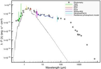
Fig. 2.SED of FT Tau. All the available photometric and spectroscopic non-simultaneous observations are plotted. The reddened
Phoenixmodel is reproducing the stellar photospheric emission (grey line). The SED clearly shows UV/optical excess emission at
wavelengths shorter than∼0.8µm and infrared excess beyond∼2µm. IRAS photometry is excluded and the higher IRAC 5.8 and 8µm photometry is omitted giving more weight to the IRS spectrum. Error bars are not visible at this scale.
Table 5.Estimated stellar properties.
Visual extinction AV 1.8±0.6 Spectral type M3±1 Effective temperature Teff 3400±200 K
Luminosity L∗ 0.35±0.09 L
Radius R∗ 1.7±0.2 R
Mass M∗ 0.3±0.1 M
Age 1.6±0.3 Myr
3.2. Disk properties
3.2.1. Disk flaring and dust composition
FT Tau shows a very prominent IR excess (see Fig. 2). By inte-grating the excess emission over the photosphere, we obtained an IR excess luminosityLIR=0.12±0.01 L.
We also measured the IR excess at different wavelengths (see Table 6) by subtracting the photospheric model from the ob-served photometry. This provides qualitative information on the geometry of the disk. As the dust grows and settles toward the mid-plane, the vertical scale height of the disk decreases, caus-ing less reprocesscaus-ing of the stellar radiation and, thus, a smaller MIR excess. According to the evolutionary scheme by Fang et al. (2009), the excess shown by FT Tau is typical of objects with disks that are evolving from amildly flaringto aflatgeometry.
The MIR spectrum of FT Tau (see Fig. 1e) shows prominent, narrow and smooth silicate features. These are thought to origi-nate in the warm, optically thin disk surface and provide infor-mation on the silicate dust in this layer. As shown by Bouwman et al. (2001) for Herbig Ae/Be stars, silicate features peaking at
∼10µm, as in the case of FT Tau, are indicative of a dust popu-lation dominated by grains as small as 0.1µm. The flattening of these features (see Furlan et al. 2006 for a large sample of TTSs) can be a tracer of the evolution of the dust population at the disk surface. Some processes such as stellar winds and radiation pres-sure can deplete sub-µm size grains (Olofsson et al. 2009). The narrow and prominent nature of the silicate features shown by FT Tau suggests that these processes are not yet efficient in this disk. The 10µm feature can also provide insight into the crys-tallinity of the silicate (e.g. Sargent et al. 2006). The absence of substructure in the MIR spectrum of FT Tau indicates that the silicates are mostly amorphous.
Finally, the MIR spectrum does not show Polycyclic Aromatic Hydrocarbon (PAH) emission features. PAH emission is indeed hardly detected in TTSs (Furlan et al. 2006), while it is common in more massive Herbig Ae/Be stars (see e.g. Meeus et al. 2001). This can be explained either in terms of different grain composition or the weaker UV radiation field of low-mass stars.
3.2.2. Disk inner radius
Most of the CO ro-vibrational lines detected with Keck/NIRSPEC are from transitions from the first vibra-tional level (ν=1−0) and their fluxes are typically a factor of a few higher than those fromν=2−1 (see Table 4).
Table 6.Infrared excess with respect to the photospheric model measured at different wavelengths. Reported errors are due to the instrumental errors and to different measurements from different observations, where available.
Wavelength (µm) Excess (mag) 3.6 0.83±0.12 4.5 1.37±0.16 5.8 1.49±0.16 8.0 2.56±0.16 24.0 5.26±0.04
-100 -50 0 50 100
Velocity (km/s)
0.8 1 1.2 1.4 1.6 1 1.2 1.4 1.6
Normalized Flux
HWZI
Telluric contamination High-J lines (J=30-40)
Low-J lines (J=1-13)
Fig. 3.Average profiles of the CO ν = 1−0 high-J (red line) and low-J (blue line) ro-vibrational lines. The green dashed line indicates the (HWZI)obsof the lines. The red and blue crosses
indicate the position ofν=2−1 blended lines.
strongly asymmetric toward the red (see Fig. 3). A likely expla-nation for this asymmetry is that most of these lines are blended withν=2−1 lines.
The disk inner radius can be estimated from the width of the CO line profile after summing over all the detected lines and correcting for the instrumental profile:
Rin=
GM∗
(∆Vobs/sini)2
'0.065·(sini)2AU (1)
whereM∗is the stellar mass,∆Vobs=65 km/s is the Half Width
at Zero Intensity (HWZI) of the CO profile, and i is the disk inclination (see Sect. 4.1.1).
3.3. Mass accretion and mass outflow rate
3.3.1. Mass accretion rate
As shown by e.g. Pringle (1981), the accretion luminosity,Lacc,
released in accretion disks or boundary layers, is related to the mass accretion rate, ˙Macc, and depends on the assumed width
[image:8.595.339.536.121.230.2]over which the emission occurs (see e.g. Bertout, Basri, &
Table 7. Accretion luminosity and mass accretion rate esti-mates from optical/NIR line luminosities and from optical ex-cess. References: (1) Fang et al. (2009); (2) Muzerolle et al. (1998c); (3) Eq. (3) of Hartigan et al. (1995).
Method Lacc M˙acc Ref. (L) (10−8M/yr)
Hβluminosity 0.09+0.11
−0.05 1.9+ 2.4
−1.1 (1) Heiluminosity 0.19+−00..7815 4.1+
17
−3.2 (1) Hαluminosity 0.17+0.26
−0.10 3.7+ 5.7
−2.2 (1) Paβluminosity 0.11+0.31
−0.08 2.4+ 6.8
−1.7 (2) Brγluminosity 0.19+1.11
−0.16 4.1+ 24
−3.4 (2) Visual excess 0.12+0.03
−0.02 2.6+ 0.6
−0.5 (3)
Bouvier 1989). In this work, we consider the accretion luminos-ity released in the impact of the accretion flow, as:
Lacc' 1−
R∗ Rin !
GM∗
R∗ M˙acc (2)
(Gullbring et al. 1998) whereR∗ and M∗ are the stellar radius and mass, andRinis the disk inner radius. We were not able to
directly measure the accretion luminosity since the UV region is only partially covered by the available observations. Therefore, we estimated the mass accretion rate by employing observed em-pirical correlations between Lacc and the luminosity of optical
and NIR emission lines which are thought to be excited in the ac-cretion columns (Fang et al. 2009, Muzerolle et al. 1998c) such as Hα, Hβ, Hei, Brγ, and Paβ(see Table 4). Furthermore, we
estimated the accretion luminosity from the visual excess with respect to the stellar photosphere as in Hartigan et al. (1995).
The derived estimates are in agreement within a factor 2, with an average value of Lacc = 0.15 L, corresponding to
˙
Macc = 3.1·10−8 M/yr (see Table 7). The largest
uncertain-ties on the estimatedLaccand ˙Maccare due to the scattering of
the empirical correlations. On the contrary, the errors onLacc
ob-tained from the visual excess are due to the continuum determi-nation and hence to the uncertainty on the estimatedAV. Further uncertainty may be due to the employed bolometric corrections.
3.3.2. Mass outflow rate
Optical and IR forbidden lines (e.g. atomic oxygen lines) are typ-ical jet tracers. Following the correlation found by Hollenbach (1985), the [Oi] 63 µm line is commonly used to constrain
the mass outflow rate (see e.g. Ceccarelli et al. 1997, Podio et al. 2012). A similar correlation has been found for the optical [Oi] 6300 Å (see e.g. Hartigan et al. 1995).
The [Oi] 63µm from FT Tau was detected only in the central spaxel (see Sect. 3). Thus, the line originates in a region around the source smaller than ∼1,300 AU and we cannot exclude a priori that a significant fraction of it originates in the disk.
Howard et al. (2013) found a tight correlation between the flux of the [Oi] 63 µm and the continuum flux at 63 µm for
Taurus sources showing no evidence of outflow. Jet sources in-stead show a line flux exceeding the value predicted by the cor-relation by up to two orders of magnitude, indicating that a sig-nificant fraction of the emission is produced in the jet/outflow.
The correlation by Howard et al. (2013) indicates that for FT Tau, up to 85% of the observed [Oi] 63µm line flux could
Table 8.Mass outflow rate estimate. References: (1) Eq. (A11) of Hartigan et al. (1995); (2) Eq. (A13) of Hartigan et al. (1995)
Method M˙W Ref.
(10−10M/yr)
[Oi] 6300 Å luminosity <7.2 (1)
[Oi] 63µm luminosity <10.7 (2)
originate in the disk. Similarly, also a fraction of the observed [Oi] 6300 Å flux could be produced in the disk. Thus, we used
the [Oi] 6300 Å and the [Oi] 63 µm line luminosity and the
correlation by Hollenbach (1985) and Hartigan et al. (1995) to derive an upper limit on the mass outflow rate ˙MW (see Table
8). We found that ˙MW<8.9·10−10M/yr. Another uncertainty
of the [Oi] 63µm flux can be source variability, since our
op-tical spectrum has been flux-calibrated through photometry (see Sect. 5.1).
4. Modeling the disk of FT Tau
To interpret the SED and the available line emission from the disk, we use the Monte Carlo radiative transfer code MCFOST (Pinte et al. 2006) and the thermo-chemical disk modeling code
ProDiMo(Woitke et al. 2009, Kamp et al. 2010) sequentially.
We fix the stellar properties as estimated from the data analy-sis (see Sect. 3.1) and run MCFOST to determine a set of dust properties that reproduces the observed SED. We perform aχ2 minimization of the SED and obtain a base set of parameters. As a second step, we run a grid ofProDiMomodels to study the behavior of predicted line fluxes by comparing the results with the observations. The results of the dust and gas modeling are discussed in Sect. 4.1 and Sect. 4.2 respectively.
4.1. Dust modeling with MCFOST
MCFOST calculates thermal and chemical properties of the dust disk by treating grains as spherical and homogeneous particles. It is based on the Monte Carlo method, allowing monochromatic photon packets to propagate through the circumstellar environ-ment. Both photospheric emission and dust thermal emission are considered as radiation sources.
As shown in Sect. 3.3.1 and Table 7, observed emission line luminosities suggestLacc values between 0.09 and 0.19 L. To
study the impact of the UV luminosity, we assumed in the mod-els an average value ofLacc=0.15 L. Then, to explore possible
variability we also assumed a value three times lower. To trans-late from accretion luminosity to fUV =LUV(90−250 nm)/L∗,
we assumed a blackbody spectrum at 10,000 K for the accretion shock. This yields fUV = 0.07 and 0.025 (in the following
de-noted as high and low fUV). In the models, the UV spectrum in
the narrow range between 90 and 250 nm is approximated by a power-lawFλ∝λpUVwithp
UV=2.0.
It is well known that pure SED modeling is highly degener-ate and thus we choose a strdegener-ategy where we fix a couple of input parameters to reasonable values, perform a crude exploration of disk scale height, dust composition, settling and inclination, and perform aχ2minimization leaving only the disk dust mass and
[image:9.595.75.264.99.154.2]optical extinction as free parameters. The fixed/explored param-eters and the results from the fitting are listed in Table 9 (see Fig. 4). Theχ2fit of the SED results in an optical extinctionAV =1.6
Fig. 4. SED predicted by MCFOST using the input parame-ters listed in Table 9 (black solid line) overplotted on the ob-served photometric points (red dots). The blue spectrum is the Spitzer/IRS spectrum.
in agreement with the result inferred by photometric colors. We obtain a disk dust mass Md = 9·10−4 M. The outer radius is
poorly constrained and we explore in the following the impact of three different outer radii, 50, 100 and 200 AU (see Sect. 5.3 for a discussion). Below, we discuss some modeling aspects and degeneracies in more detail.
4.1.1. Disk inclination and extent
Guilloteau et al. (2011) derived an inclination of 23±14◦from CO sub-millimeter line kinematics. However, the performed SED modeling indicates that for a disk inclination i < 30◦, the predicted SED has a NIR bump considerably lower than ob-served. On the other hand, if the inclination isi>75◦, the photo-spheric emission is shielded too much by the disk. We found that the SED is well reproduced fori =60◦. However, a fine-tuning
of this parameter is hardly feasible and the degeneracy between inclination and inner radius (arising from the analysis of the CO lines, see Sect. 3.2.2) remains unsolved (see Appendix A).
Assuming an inclination of 60◦, the disk inner radius inferred from the profile of the CO ro-vibrational lines isRin=0.05 AU
(see Eq. 1). The estimated disk inner radius is at '6.3 R∗, in agreement with estimates of the magnetic truncation radius for typical CTTSs (Shu et al. 1994, Donati et al. 2008, Long et al. 2011).
The outer radius of the disk is poorly constrained by the SED. Models with Rout = 50, 100, and 200 AU (all other
pa-rameters kept constant) result in the same SED within the pho-tometric error bars (see Sect. 5.3 for a more detailed discussion).
4.1.2. Dust grain composition
The 10µm silicate feature suggests that sub-µm size dust grains are still present in the surface layer of the disk (see Sect. 3.2.1). The mineralogy used in our models is amorphous MgFeSiO4
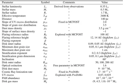
Table 9.Parameters of the FT Tau model. The difference between an ‘explored’ and ‘free’ parameter is that the former is set after an exploratory parameter study while the latter is derived usingχ2fitting of the SED.
Parameter Symbol Comments Value
Stellar luminosity L∗ Derived from observations 0.35 L
Stellar mass M∗ ” 0.3 M
Stellar radius R∗ ” 1.7 R
Effective temperature Teff ” 3400 K
Distance d ” 140 pc
Slope of UV excess distribution pUV Fixed in MCFOST 2.0 Slope of grain size distribution apow ” 3.5
Dust mass density ρd ” 3.5 g cm−3
Slope of surface mass density ” −1
Flaring reference radius R0 Explored with MCFOST 100 AU Flaring reference height H0 ” 12, 14 AU (high/lowfUV)
Flaring exponent β ” 1.15
Disk inner radius Rin ” 0.09, 0.05 AU (high/lowfUV) Minimum dust grain size amin ” 0.05, 0.1µm (high/lowfUV)
Maximum dust grain size amax ” 1 cm
Stratification exponent sset ” 0.2, 0.3 (high/lowfUV) Stratification grain dimension aset ” 0.05, 0.1µm (high/lowfUV)
Inclination i ” 60◦
Disk outer radius Rout ” 50, 100, 200 AU
Optical extinction AV Free parameter in MCFOST 1.6
Disk dust mass Md ” 9·10−4M
Cosmic Ray Ionization rate ζ Fixed inProDiMo 1.7·10−17s−1 UV excess fUV Explored withProDiMo 0.07, 0.025
PAH abundance fPAH ” 10−2,10−3,10−4
Disk gas mass Mg ” (9, 4.5, 1.8)·10−2M
line profiles (Rin = 0.05 AU, see Sect. 3.2.2 and above). If we
assume that the dust and gas inner radii are coincident, the dust temperature at that radius has to be below the sublimation tem-perature. Thus, grains with a < 0.1µm cannot survive at that
radius and we useamin =0.1 µm. Another possibility is that a
fraction of the CO ro-vibrational line emission originates from gas inside the dust sublimation radius. amax is not well
con-strained and degenerate with the slope of the grain size distri-bution. Thus, we useamax =1 cm, which is a typical value for
disks at this stage. The high fUVmodel requires a slightly larger Rin of 0.09 AU and has a slightly smaller minimum grain size,
amin=0.05µm.
4.1.3. Disk flaring and dust settling
The surface mass density of the disk is parametrized as
Σ∝r− (3)
and the disk scale height as
H(r)=H0· r R0
!β
(4)
withrbeing the distance from the star andH0the disk height at
the reference radiusR0. According to the qualitative analysis of
the IR excess in Sect. 3.2.1, the disk is mildly flared and we thus fixed the flaring angle to beβ=1.15. The best fit resulted in a scale height ofH0 =12 AU and H0 =14 AU for the high and
low fUVrespectively atR0=100 AU. Smaller scale heights lead
to an underprediction of the FIR fluxes.
Dust settling is parametrized assuming that the scale height changes with grain size for grains larger thanaset
H(r,a)=H(r)·(a/aset)−sset/2 (5)
The best match of the observed silicate features is found by in-cluding dust settling with all particles involved, i.e. aset=0.05
µm, and an exponentsset=0.2.
4.2. Gas modeling with ProDiMo
ProDiMocalculates the chemistry and heating/cooling of the gas
self-consistently using a large chemical network of 111 species and 1462 reactions. An extensive list of all heating and cool-ing processes can be found in Woitke et al. (2009, 2012). In this work, we do not feed the gas temperatures back into the verti-cal hydrostatic equilibrium, but instead keep the vertiverti-cal flaring structure given by the MCFOST parametrization found for the best fitting SED model. Using the results from the MCFOST models described in the previous section, we ran a small grid of
ProDiMomodels with different values of UV excess, gas mass
and PAH abundance.
Two UV excess cases were considered (high state, fUV =
0.07, and low state fUV =0.025, see Sect. 4.1). We fixed Mdust
as suggested by MCFOST and explored dust-to-gas mass ratios of 0.01, 0.02, and 0.05, i.e. Mgas=0.090, 0.045, and 0.018 M
(hereafter denoted as hGAS, iGAS, and lGAS). Even the most massive model with Mgas=0.09 M is gravitational stable
ac-cording to the Toomre criterion (see Eq. A.10 of Kamp et al. 2011). The abundance of PAHs, fPAH, was set to 10−2,10−3, and
10−4times the one in the ISM (hereafter denoted as hPAH, iPAH,
and lPAH). The combination of these three parameters yields a total of 18 disk models.
The level populations for the line radiative transfer are cal-culated from statistical equilibrium and escape probability (see Woitke et al. 2009, for details). Using these populations, we carry out a detailed line radiative transfer using ray tracing and taking into account the disk rotation and inclination (Woitke et
Fig. 5.From top to bottom, left to right: the total hydrogen number density, the dust temperature, the gas temperature, and the CO abundance distribution in the reference disk model, namely the case with low UV excess, low gas mass, and low PAH abundance. The black contours indicate the total AV=0.1,1 lines. The white contours indicate the gas temperature, while the red contours in
the dust temperature plot indicate dust temperature.
al. 2011, Appendix A.7). These detailed radiative transfer fluxes for the eighteen models are listed in Table 10: the [Oi] 63µm
line and three representative CO ro-vibrational lines,ν=1-0 P4, P36, andν=2-1 P4.
We chose as a reference model the lUV, lPAH, lGAS one. Fig. 5 illustrates the density and temperature distribution (dust and gas) as well as the CO abundance in that particular model. The dust and gas temperature are well coupled in the region with
AV>1. The CO abundance reaches a maximum value of∼10−4
already well above that line and the top CO layer resides at tem-peratures above 1000 K inside 10 AU. Since the CO fundamen-talν=1−0 ro-vibrational lines are optically thick, they largely originate in this hot surface layer (see also Fig. 6). The main heating process in this region is PAH heating and collisional de-excitation of H2. The main cooling processes are CO rotational
and ro-vibrational line cooling as well as water line cooling.
4.2.1. The CO ro-vibrational lines
We use in this study the large CO model molecule compiled by Thi et al. (2013) including IR and UV pumping. The model uses
7 vibrational levels of the X1Σ+and A1Πelectronic states and
60 rotational levels within each of them. ProDiMo calculates the level populations from statistical equilibrium and performs a detailed line radiative transfer to obtain the emerging CO line fluxes (Woitke et al. 2011). This type of thermo-chemical model-ing leaves no freedom to adjust CO densities, column densities, densities of collision partners or gas temperatures.
The ProDiMo models show that CO ro-vibrational line
fluxes are very weakly affected by the PAH abundance while they substantially correlate with the gas mass (Table 10). Models with high UV excess generally over-predict the observed fluxes (up to a factor 15). However, those with low gas mass well re-produce or slightly over-predict (by a factor 2) allν=1−0 line fluxes. All models with low UV excess agree fairly well with the ν = 1−0 and over-predict up to a factor 5 theν =2−1 line fluxes (see Fig. 7).
Alternatively, we also calculated the expected CO line fluxes from a simple line synthesis calculation (see Najita et al. 1996 and Brittain et al. 2009 for an extensive description). We as-sumed that the emission arises from a vertically isothermal slab of gas with constant column density (N =2·1018 cm−2). The
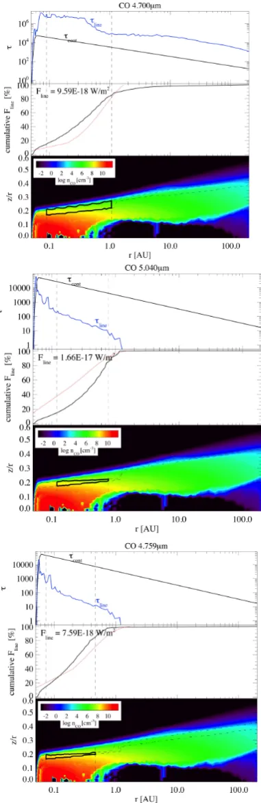
rep-Fig. 6.Cumulative flux distribution from vertical escape proba-bility in aProDiMomodel with low UV excess, low gas mass, and low PAH abundance. The top panel of each box shows the vertical optical depth for the line and continuum. The middle panel of each box shows the cumulative flux from theProDiMo
model (black) and best fit slab model (red). The bottom plot of each box shows the CO density distribution in the disk. Outlined with black contours is the region in which radially and vertically between 15 and 85% of the flux originates. The top box is for theν=1−0 P4 line, the middle box for theν=1−0 P36 line, the bottom box for theν=2−1 P4 line.
resentative collision partner. The rotational levels are assumed to be thermalized while vibrational populations are calculated explicitly. From χ2 minimization, we find a hydrogen volume density profile nH(r) = 1.5·1014 (r/Rin,slab)−2 cm−3 and a gas
temperature profileT(r)=1200 (r/Rin,slab)−0.55K. The inner
ra-diusRin,slabis only loosely constrained to 0.1+−00..107 AU, because
the line wings have a rather low S/N. The outer radius is largely unconstrained due to the degeneracy between the surface density of the gasNand the outer radius of the emitting area;Rout,slabhas
to be larger than 0.9 AU. The turbulent line broadeningbis found to be 2 km/s, althoughNandbare degenerate. The gas tempera-ture found at the inner radius isT0=1200+−300200K. Integrated line
fluxes have been measured from the spectrum generated with the slab model in the same way as for the observed spectra. The model predicts correctly theν =1−0 lines and theν =2−1 lines withTex∼6200 K. However, theν=2−1 lines at higher
energy are over-predicted by a factor 5 (see Fig. 7). This could indicate that the gas is more diffuse (lower volume density), that the line flux declines steeper with distance from the star (steeper density power-law), or that some additional non-LTE effects are still missing in the slab model.
Fig. 6 shows the cumulative flux distribution from simple vertical escape probability in the lUV/lPAH/lGAS ProDiMo
model for the three representative lines, ν=1-0 P4, ν=2-1 P4, andν=1-0 P36. The CO lines are sub-thermally excited; in the hUV/lPAH/lGAS model, the three lines studied here as repre-sentative lines are a factor 2-3 lower than their respective LTE values. The agreement betweenProDiMomodels and the more simple slab models on how the flux is building up as a function of radius is very good (see comparison in Fig. 6). TheProDiMo
models also show a similar temperature of∼1000 K at the inner radius of the CO ro-vibrational line emitting region (compared to 1200 K from best fit slab model).
It turns out that the CO line fluxes depend on gas mass, UV excess, and PAH abundance (see Table 10). Hence, the lines can-not be used to directly constrain the disk gas mass. The appar-ently better fit of the simple CO line modeling could be largely due to the fact that parameters such as CO column density, gas temperature and collision partner density can be varied indepen-dently without imposing a self-consistent disk structure. This means that CO in a slab model can for example exist in re-gions where it would be photodissociated in a thermo-chemical disk model, thus allowing UV fluorescence to affect the CO ro-vibrational lines much stronger in the former case. Another pos-sibility could be that part of the CO ro-vibrational emission orig-inates from gas inside the dust sublimation radius of our models. At this stage, a further analysis of these CO ro-vibrational lines is largely limited by the observations, which have limited spec-tral resolution and suffer from a low signal-to-noise and telluric contamination (see Sect. 2.4).
4.2.2. The [Oi] 63µm line
As shown in Table 10, the [Oi] 63µm line flux is affected by the
UV excess, the gas mass, and the PAH abundance. Differences of a factor two are found between the high and low UV excess models. The dependence on the gas mass stems from the fact that the gas temperature changes with disk mass and, in turn, affects the line flux. The fact that the flux increases with PAH abundance is explained by the increasing photoelectric heating of the gas in the upper disk layer (Jonkheid et al. 2004). Thus, gas mass, UV excess and PAH abundance are to some degree degenerate in the prediction of the [Oi] line flux.
[image:12.595.72.263.57.644.2]0 1 2 3 4 5 6 7 8 9 10 11 29 30 31 32 33 34 35 36 37 38 39 J
-71 -70 -69 -68 -67 -66
ln(F/vA(2J+1))
High UV/High Gas Model High UV/Intermediate Gas Model High UV/Low Gas Model Low UV/High Gas Model Low UV/Intermediate Gas Model Low UV/ Low Gas Model Slab Model Observed 1-0 Observed 2-1
1 2 3 4 26 27 28 29
J
[image:13.595.68.542.57.231.2]-74 -73 -72 -71 -70 -69 -68
Fig. 7.Rotational diagram of CO ro-vibrational lines observed (left:ν=1−0, right:ν=2−1) versus model predicted: slab model described in the text andProDiMoruns with intermediate PAH abundance, with high, intermediate, and low gas mass, and with high and low UV excess. The vertical dotted lines indicate discontinuity in the x-axis.
Table 10.Fluxes of the [Oi] 63µm line and of three
representa-tive CO ro-vibrational lines as predicted by the grid ofProDiMo
models using detailed line radiative transfer, the slab model de-scribed in the text, and as observed.
Model Flux (10−17W/m2)
[Oi] CO CO CO
UV/PAH/GAS 63µm 1-0 P4 2-1 P4 1-0 P36
h/h/h 30.4 6.51 5.07 10.4
h/i/h 21.7 5.10 4.79 10.3
h/l/h 20.9 4.95 4.77 10.3
h/h/i 24.7 4.35 2.99 7.05
h/i/i 18.3 3.55 2.86 6.95
h/l/i 17.7 3.41 2.84 6.59
h/h/l 17.5 2.11 1.31 3.09
h/i/l 13.4 1.81 1.26 3.02
h/l/l 12.9 1.77 1.25 3.02
l/h/h 15.6 2.97 2.03 5.31
l/i/h 11.3 2.17 1.80 5.05
l/l/h 10.8 2.08 1.78 5.03
l/h/i 13.1 1.94 1.15 3.04
l/i/i 9.92 1.44 1.06 2.91
l/l/i 9.59 1.38 1.05 2.90
l/h/l 10.1 1.03 0.55 1.26
l/i/l 7.99 0.79 0.52 1.21
l/l/l 7.77 0.77 0.52 1.20
Slab model - 1.25 0.40 1.31
Observed 1.6±0.5 1.65±0.38 0.28±0.10 0.83±0.08
5. Discussion
In this section, we discuss the source variability and the results of our detailed disk modeling in the context of the available ob-servational data.
5.1. Source variability
Young circumstellar systems are often highly variable objects (see e.g. Bouvier et al. 1993). Flux variability up to a factor∼3
has been measured for FT Tau in the V band on a timescale of five years (ASAS, Pojmanski 2002). Furthermore, flux variabil-ity up to a factor∼2.8, 2.1, and 1.3 has been measured in B, V, and I band respectively on a timescale of 45 days (Fern´andez, private comm.) with the SITe CCD attached to the 1.23 m tele-scope of the Calar Alto Observatory (Almer´ıa, Spain). The anal-ysis of this variability revealed that it cannot be reproduced by cold spots in the stellar photosphere because the amplitude of the variations observed in the V band is too large with respect to variations in the I band. On the contrary, these amplitudes are well matched by photospheric hot spots (from 5000 to 6600 K) if we assume the effective temperature of M3 stars. The B band shows an amplitude slightly smaller than expected for those hot spots but this can be explained by the presence of a hot contin-uum in addition to the pure photospheric emission.
Given this, the brightness at the minimum of the light curves provides an upper limit to the photospheric brightness of the star. As we see from Fig. 8, the reddened photospheric emission in the V band assumed in Sect. 3.1 is lower than measurements, from either ASAS or Calar Alto surveys. This indicates that the extinction cannot be much lower than estimated in Sect. 3.1, be-cause this would increase the reddened photospheric emission of the model to values higher than the observed one. The USNO V band photometry used to flux-calibrate the TNG spectrum (and, thus, to estimate the mass accretion rate, see Sect. 2.1 and 3.3.1) turns out to be an average value of all measurements (see Fig. 8). In order to address the origin of the observed variability, a time-dependent study of optical/NIR emission lines is necessary. Any relation between these lines and contemporary observations of optical photometric variations can clarify if and how much of the observed variability is due to the accretion process. In addition, we must be careful in the interpretation of line emission from the disk surface especially if these lines result from UV pumping by stellar radiation.
5.2. The CO ro-vibrational lines
[image:13.595.42.303.370.616.2]of this hot surface and it can change due to the particular choice of the dust opacities, the scale height of the disk and the flaring. The quality of the available Keck CO ro-vibrational line profiles is not good enough to derive the extent of the hot surface layer directly from their shape. In case of exquisite data quality, this can be done as shown by Goto et al. (2012) for the example of HD100546, a Herbig Ae star. So, as new data will become avail-able, these parameters should be refined keeping the constraints on the SED.
5.3. The [Oi] 63µm line
All models presented here over-predict the [O i] 63 µm line.
Since the line is optically thick, its flux is mostly affected by the gas temperature in the emitting region and the total emitting surface area. The models indicate that the [Oi] 63µm line typ-ically originates between∼ 10 and 200 AU. Roughly 15% of the total line flux builds up between 100 and 200 AU. In order to understand the dependence of the predicted [Oi] line flux on
the adopted disk size, we calculated models with different outer radii (50, 100, and 200 AU, see Table 9). We find that the line flux decreases by only a factor 4 for the smallest disk size. This is due to the fact that the smaller emitting area is partially com-pensated by the higher gas temperature of the emitting region. At the same time, the CO ro-vibrational lines do not change within the modeling uncertainties. Hence, the observed emission lines do not allow us to put any stronger constraint on the size of the gaseous disk.
Guilloteau et al. (2013) derive from IRAM 30-m CN N=2−1 observations an outer radius of 310 AU. Previously, a simple power law disk model fit to 1.3 mm and 2.7 mm interferometric continuum data yieldedRout = 57 AU
(Guilloteau et al. 2011). However, the disk is barely resolved and better interferometric images at shorter wavelength are required to measureRout for the dust; at the same time, interferometric
line data e.g. for CO isotopologues are required to obtain a reliable outer gas radius. Previous work shows that gas and dust outer radii at submm wavelength can actually differ (e.g. Isella et al. 2007, Andrews et al. 2012). Given the existing uncertainty on the estimate ofRout, models with different gas and dust outer
radii have to await better observational data.
In the region where the [Oi] 63µm line emits, photoelectric
heating is one of the dominant heating processes. Since the PAH features are not observed in the Spitzer spectra, their abundance can be arbitrarily low. Supressing the PAH abundance even be-low the be-lowest value in the grid, fPAH = 10−4, does not affect
the [Oi] line flux anymore. A lower disk gas mass shifts the line forming region to lower depth in the disk, thus making the line flux weaker.
6. Summary
We have performed analysis and modeling of the SED and emission lines of the TTS FT Tau to fully characterize the stellar, disk, and accretion properties. We reduced and anal-ysed five spectra from optical to FIR wavelengths, taken with the optical Telescopio Nazionale Galileo, the NIR William Herschel Telescope, the NIR Nordic Optical Telescope, the high-resolution NIR Keck Observatory, and the FIRHerschelSpace Telescope. Additional data were retrieved from the literature and consist of a MIR Spitzer Space Telescope spectrum and of 44 photometric measurements from optical to radio wavelengths. We studied a set of models of the source generated by means of
the radiative transfer code MCFOST and the thermo-chemical disk modeling codeProDiMo.
We found that FT Tau is a low-mass (0.3±0.1 M) and
-luminosity (0.35±0.09 L) M3 star showing very high
vari-ability (probably due to photospheric hot spots). The estimated properties are typical of young unevolved systems in the Taurus star forming region with ages of roughly 1 Myr. The optical ex-tinction (AV =1.8) is also within the range of typical values in Taurus.
The inner radius of the circumstellar disk is small (0.05+0.04
−0.02 AU) indicating an early stage of internal disk
dis-sipation. This is in agreement with the fact that the source is strongly accreting. In fact, the derived mass accretion rate ((3.1±0.8)·10−8M/yr) is a high value for M-stars, since this
corresponds toLacc∼0.4L∗. The ratio of mass outflow to mass
accretion rate is lower than 0.03, in agreement with typical ob-served values for TTSs (Hartigan et al. 1995). The disk is quite massive (∼0.02 M) with respect to the stellar mass (mass ratio ∼0.06). Small silicate grains are still present in the disk surface even though at lower abundance due to some degree of settling. Winds and radiation pressure seem to be inefficient at removing this small grain population. These findings are consistent with the apparent primordial nature of this disk (e.g. no gaps, holes). The PAH abundance is inferred to be extremely low (∼ 10−4
times that in the ISM).
From this work it is clear that FT Tau can be considered as benchmark for primordial disks in the Taurus molecular cloud with high mass accretion rate, high gas content, and typical disk size. It is an interesting target for follow-up chemical studies as well as for informing surveys of star forming regions on more prototypical objects to expect.
Acknowledgements. We acknowledge the referee for valuable comments that considerably improved the paper. We thank Matilde Fern´andez and Victor Terr´on for observing FT Tau and reducing the data at the Calar Alto Observatory. We really appreciate the helpful discussion about the origin of the variability. We also gratefully thank Gwendolyn Meeus for her work in acquiring data with the TNG and Ilaria Pascucci and Veronica Roccatagliata for reducing the data from Spitzer. This work is supported by the Swiss National Science Foundation. LP acknowledges the funding from the FP7 Intra-European Marie Curie Fellowship (PIEF-GA-2009-253896). IK, WFT, FM, and PW acknowledge funding from an NWO MEERVOUD grant and from the EU FP7- 2011 under Grant Agreement nr. 284405. FM acknowledges support from the Millennium Science Initiative (Chilean Ministry of Economy), through grant Nucleus P10-022-F. I. Pascucci acknowledges NASA/ADP Grant NNX10AD62G. This research has made use of the SIMBAD database, operated at CDS, Strasbourg, France.
Appendix A: Uncertainties of the analysis
In this appendix we discuss the limitations of our analysis due to non-simultaneous observations and quantify thoroughly the uncertainties on the inferred results.
The mentioned stellar variability does not have strong impact on the determination of the stellar properties because it does not affect significantly the shape of the optical spectrum (used to determine the spectral type) and the J and H band fluxes (used to estimate luminosity and radius).
On the contrary, the estimate of the visual extinction is af-fected by large uncertainties. We firstly remark that the use of the (J-H) color as tracer of the extinction relies on the assump-tion that the observed flux at those wavelengths is entirely emit-ted by the stellar photosphere. Secondly, the determination of the optical extinctionAV is pretty sensitive to the surface grav-ity of the assumed model. By varying the stellar radius or mass by 30%, we obtain AV values between 1.2 and 2.5. This may add a further factor 15% uncertainty to the estimates of stellar
2500 3000 3500 4000 5900 5925 5950
Time (HJD-2450000)
14
14.5
15
15.5
Magnitude
Calar Alto survey ASAS survey [image:15.595.83.526.60.306.2]USNO photometry (used in this work) Photospheric emission (assumed in this work)
Fig. 8.ASAS, Calar Alto, and USNO photometric measurements of FT Tau in the V band. The dashed line indicates the reddened photospheric magnitude assumed in our analysis. The vertical line indicates a gap in the x-scale. The position in time of the USNO photometry is arbitrary.
properties. However, the fact that the accretion luminosity val-ues estimated by using different tracers from 0.45 and 2.17µm does not show a dependence with the wavelength (see Fig. A.1) is a strong sanity check for the determination of AV. The fact that we find the sameAVvalues by using two independent meth-ods (the observed colors, Sect. 3.1, and the modeling approach, Sect. 4.1) further reinforces our result. The large difference be-tween our estimate of the stellar luminosity and the result from Rebull et al. (2010) (see Table 1) is due to the determination of
AVwhich is in turn due to the assumed surface gravity.
The spectral type-Teff relation can actually introduce an
ad-ditional error. Differences up to some hundreds of Kelvin arise for M-type stars among different works (see e.g. Da Rio et al. 2010). Finally, further uncertainty in the determination of the stellar properties is provided by the PMS star tracks adopted to infer the stellar mass and age. Hartmann (2001) suggested that the age spread inferred for TTSs in Taurus may exclusively be due to uncertainties towards individual members.
In Sect. 3.2.2 we estimated the disk inner radius by measur-ing the width of the CO ro-vibrational lines. The largest uncer-tainty in the determination ofRin is set by the adopted inclina-tion. The width of the CO lines is equally reproduced by config-urations with (i:Rin)=(60◦ : 0.05 AU), (45◦ : 0.03 AU), and
(30◦: 0.02 AU).
The estimates of the mass accretion and outflow rate may be affected by variability, since the optical and NIR spectra used to measure the line luminosities were flux-calibrated by using non-simultaneous photometry. This is particularly true for esti-mates based on optical lines (optical flux variability∼2.1, see Sect. 5.1). The variability implies uncertainties on the estimates of the accretion luminosity in addition to the scattering of the empirical correlations employed to deriveLacc(Sect. 3.3.1). The
lowest and the highest estimates for Lacc have been found by
means of emission lines from the same spectrum (thus taken si-multaneously, see Table 7). This is indicating that the scattering
Hβ 0.45 He I 0.58 Hα 0.65 Paβ 1.28 Brγ 2.17 -2
-1 0 1
log (Accretion luminosity) (L
⊙
) Visual extinction = 0.0
Visual extinction = 1.8 Visual extinction = 4.0
Fig. A.1.Accretion luminosity estimated from the luminosity of emission lines at optical to NIR wavelengths (x-axis) for diff er-ent AV values. The grey stripe indicates the range of values in-ferred from the Brγline, which is the least affected by extinction. It is clear the trend with wavelength for high and no extinction. Slight displacement between points has been put for a better vi-sualization.
of the empirical relations might play the major source of uncer-tainty on the accretion luminosity.
References
Andrews, S. M., & Williams, J. P. 2005, ApJ, 631, 1134 Andrews, S. M., & Williams, J. P. 2007, ApJ, 659, 705
Andrews, S. M., Wilner, D. J., Hughes, A. M., et al. 2012, ApJ, 744, 162 Aspin, C. 1999, Astrophysics with the NOT, 29
Basri, G., & Bertout, C. 1989, ApJ, 341, 340
[image:15.595.316.549.378.519.2]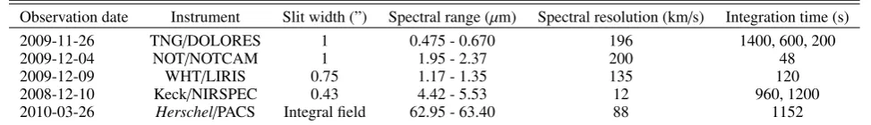
![Fig. 1. Spectroscopic observations. (a) TNG optical spectrum; (b) WHT J-band spectrum; (c) NOT K-band spectrum; (d) Keckhigh-resolution spectra; (e) Spitzer MIR spectrum; (f) Herschel FIR spectrum of the only detected line ([O i] 63 µm); (d1) and(d2) zoom](https://thumb-us.123doks.com/thumbv2/123dok_us/8744594.388700/4.595.106.503.50.734/spectroscopic-observations-spectrum-keckhigh-resolution-spitzer-spectrum-herschel.webp)