R E S E A R C H A R T I C L E
Open Access
Coupling dynamical and statistical
downscaling for high-resolution rainfall
forecasting: case study of the Red River
Delta, Vietnam
Quan Tran Anh
1*and Kenji Taniguchi
2Abstract
The hybrid dynamical-statistical downscaling approach is an effort to combine the ability of dynamical downscaling to resolve fine-scale climate changes with the low computational cost of statistical downscaling. In this study, we propose a dynamical-statistical downscaling technique by incorporating a regional climate model (RCM) with artificial neural networks (ANN) to downscale rainfall information over the Red River Delta in Vietnam. First, dynamical downscaling was performed with an RCM driven by the reanalysis to produce nested 30- and 6-km resolution simulations. Subsequently, the 6-km simulation was compared to rain gauge data to examine the ability of the RCM to reproduce known climate conditions. Then, in the statistical downscaling step, the ANN was trained to predict rainfall in the 6-km domain based on weather predictors in the 30-km simulation. Statistical downscaling results were compared with the original output from RCM to determine the accuracy of the coupling method. A bias correction method to locate no-rainfall events in the ANN downscaling result was also developed to enhance the credibility of the final results. The outcomes of this study illustrate that ANN can produce RCM-like results (r> 0.9) at a fraction of the cost, with an 89% reduction in the required
computational power.
Keywords:Dynamical downscaling, Statistical downscaling, ANN, WRF, Rainfall
Introduction
Rainfall is one of the most important meteorological phenomena on Earth. It not only provides a vital fresh-water source supporting all lifeforms, but also causes various types of natural disasters such as floods, land-slides, storms, and drought. It is important to have a deep understanding of the rainfall formation mechanism to forecast the timing, density, intensity, and trends in a specific region to better manage water resources, maximize the use of water for economic development, and minimize the impacts of extreme events. In many countries, including Vietnam, rainfall is the object of re-gional planning strategies involving the production and construction sectors. Since the efficiency of water resource management depends on the accuracy and detail of
rainfall forecasts, a method to obtain reliable and accurate predictions of rainfall at high spatial resolution is indis-pensable (Arritt and Rummukainen 2011; Caldwell et al. 2009; Giorgi and Mearns1991).
Multiple general circulation models (GCMs) have been developed by various research groups to provide future climate predictions using numerical weather simulation. GCMs represent the physical processes and feedbacks for the atmosphere and oceans, which can be used to forecast future climate changes. Although GCM models can make useful predictions about global large-scale climate indicators, their spatial resolution of 100– 200 km are too coarse to satisfy the requirements of regional planning. A GCM simplifies the complexities of land-sea distribution, vegetation cover, topography, and terrain. Therefore, downscaling methods, which translate coarse-scale GCM to finer spatial scales, have been developed to use on limited-area domains at higher hori-zontal resolutions.
* Correspondence:[email protected]
1School of Natural Science and Engineering, Kanazawa University, Kakuma-machi, Kanazawa 920-1192, Japan
Full list of author information is available at the end of the article
Dynamical downscaling works by employing a regional climate model (RCM), which is based on the same prin-ciples as a GCM but has higher resolution over a limited area. An RCM uses large-scale atmospheric conditions as determined by a GCM for the lateral boundary condi-tions. Higher resolution topography and land-sea distri-bution are incorporated to generate realistic climate information at a much finer spatial resolution (Seaby et al. 2013). Currently, RCMs are considered the most helpful method for producing climate information at the scales required for actionable strategic planning (Kjell-strom et al.2016).
Over the years, the applicability of dynamical down-scaling has significantly improved owing to the continu-ous development of computing technology and advances in numerical models. Even though the use of dynamical downscaling has become easier, it continues to be an ex-tremely demanding method that requires considerable computational cost, simulation time, and output storage. Statistical downscaling is an alternative to dynamical downscaling for high-resolution climate downscaling that can overcome the drawbacks of dynamical down-scaling methods. Statistical downdown-scaling takes into ac-count the empirical, spatial, and temporal relationships between large-scale climate indicators (predictors) and local-scale climate variables (predictands) and are trained on a historical period. Subsequently, these rela-tionships are presumed to hold in the future, where they can be used to determine future predictands. Statistical downscaling methods are computationally inexpensive and significantly faster than dynamical downscaling, so they can be applied for even higher resolutions, up to station-scale. Since statistical downscaling methods rely on the assumption of an unchanged statistical relation-ship, they require long historical climate observation data for validation, which is not always available for every region. In contrast, dynamical downscaling oper-ates based on physical realism with complex local pro-cesses, which allows it to map important fine-scale variations in climate that otherwise might not be in-cluded (Salathé Jr et al. 2008; Pierce et al. 2012; Walton et al.2017).
While statistical downscaling and dynamical downscal-ing methods are widely used in climatology research, both face drawbacks that limit their applicability. Re-cently, the approach of combining dynamical downscal-ing with statistical downscaldownscal-ing has been explored. Dynamical-statistical downscaling is a blended tech-nique, where an RCM model is initially adopted to downscale the GCM output followed by the application of statistical formulas to further downscale the RCM output to a higher resolution. Dynamical downscaling methods can utilize the advantages of RCM to provide better predictors for use in statistical downscaling
(Guyennon et al.2013). Berg et al. (2015) demonstrated this promising method by using a hybrid of the weather research and forecasting (WRF) model with the empir-ical orthogonal function to effectively forecast precipita-tion changes. In other research, Walton et al. (2015) introduced a new dynamical-statistical downscaling method by coupling WRF with principal component analysis. The statistical-dynamical downscaling method is another approach for blending techniques where dy-namical downscaling is applied after a selected statistical downscale. While statistical-dynamical downscaling is a more complex blending technique, it is computationally less expensive. These methods use a statistical approach to refine the GCM outputs into a few characteristic states, which can be later used with the RCM models (Fuentes and Heimann2000).
Limited efforts have been made to date to combine dy-namical and statistical downscaling methods for precipi-tation research. In this study, we have introduced a combined dynamical-statistical downscaling technique for rainfall using WRF with an artificial neural network (ANN). The WRF-ANN method aims to downscale high-resolution daily rainfall data for a seasonal length to satisfy the requirements for purposes such as agricul-ture or water resources planning. This method works by making statistical relationships between moderate- and high-resolution WRF outputs using ANN. The statistical relationships can be used directly to downscale moderate-resolution WRF outputs to fine-resolution rainfall. In this method, we first validated the accuracy of the WRF model to reproduce known climate condi-tions. Subsequently, the WRF output was downscaled to a finer spatial resolution using ANN. While this method used atmospheric variables from WRF, the relationship between physical and dynamical processes could poten-tially be included in the ANN. In addition, a bias correc-tion for the ANN input and output (rainfall) was applied to reduce error in the final output. Moreover, the sensi-tivity of each predictor was also considered to examine their statistical relationships with rainfall.
Methods/Experimental Numerical weather simulation
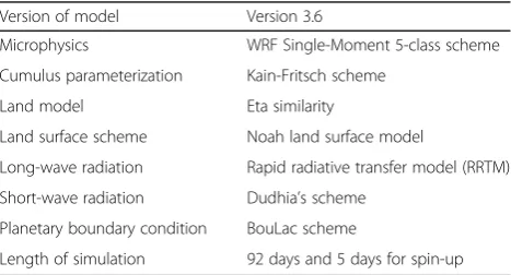
WRF has a wide range of physical options for parameterization, which can be combined in various ways. In the context of this study, the physical parameterization settings were selected based on the op-timal combination of schemes used in various studies across Asia. Cloud microphysics was used from the WRF Single-Moment 5-class scheme (Hong et al.2004). The Kain-Fritsch scheme was used for cumulus parameterization. For surface layer physics, the ETA models based on Monin-Obukhov, with a Carlson-Boland viscous sub-layer, were used. As a land surface model, the Noah land surface model (Chen and Dudhia 2001) was applied. The Bougeault and Lacarrere (Bou-Lac; Bougeault and Lacarrere1989) scheme was used for the planetary boundary layer. Dudhia’s scheme (Dudhia 1989; Mlawer et al.1997) and the rapid radiative transfer model (RRTM) were selected for short- and long-wave radiation conditions, respectively. The spectral nudging option was enabled to include global-scale effects at a smaller scale to ensure the simulated result would be more consistent with observations (Storch et al. 2000). An outline of the model configuration is provided in Table1.
Since this research focuses on the rainfall season, dy-namical downscaling was applied to each JJA period of the research duration. For the initial and boundary con-ditions, downscaling simulations used JRA-55, NCEP-FNL, and NOAA OI SST datasets. The research area used for downscaling by WRF is shown in Fig.1a. The two-domain nesting method was applied with 30- and 6-km horizontal grid resolutions for the outer and inner domains, respectively (hereafter, D1 and D2). While D1, placed in Southeast Asia, covers the entire Vietnam re-gion, D2 was selected over the northern part of the country. D2 has complex topography, including alternat-ing mountain ranges, midlands, lowlands, and a small section of the East Sea (Fig.1c). The target area for pre-cipitation estimation using ANN was placed inland in-side D2 (hereafter, D2T; Fig.1b), between latitudes 20.5° N–22.5 °N and longitudes 104°E–107°E, covering the large Red River Delta region and Hanoi City, the capital.
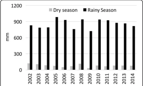
The area defined by D2T is not only the most important municipal area in Vietnam, but it also has the longest and most reliable climatological records. The weather in northern Vietnam is characterized by the tropical cli-mate system (Fig.2) and is distinguished by a hot, rainy season from Jun to August (JJA) followed by a cold, dry season from December to February (DJF). The average rainfall during JJA ranges from 750 to 1100 mm, which accounts for over 70% of the annual precipitation. Rain-fall is a vital water source for development in the region and also the cause of many disasters. In this study, we focused on precipitation during the JJA period.
The goal for the WRF model was to accurately repro-duce detailed information about rainfall in the D2T. Here, we evaluate the ability of WRF to reproduce daily rainfall by comparing model output to surface observa-tion data (see Fig.1c) for the spatial distribution of rain gauges). The downscaling experiments were imple-mented for each JJA period in 1996, 1997, 1998, and 2006. While evaluating the reproducibility of the WRF model, we omitted the results from the first 5 days, allowing a spin-up period from May 27 to May 31. After the spin-up period, the 92-day simulation was carried out from the first day of June to 18Z (midnight local time) on August 31. Model performance was evaluated by computing a series of statistical measures for simu-lated rainfall against observed rainfall, including the mean absolute error (MAE), Pearson’s correlation (R), root mean square error (RMSE), and index of agreement (IOA). The statistical measures were defined as follows:
MAE¼ 1
N
XN
i¼1jOi−Sij ð1Þ
R¼
PN i¼1 Oi−O
Si−S
ffiffiffiffiffiffiffiffiffiffiffiffiffiffiffiffiffiffiffiffiffiffiffiffiffiffi PN
i¼1 Oi−O
q ffiffiffiffiffiffiffiffiffiffiffiffiffiffiffiffiffiffiffiffiffiffiffiffiP
M i¼1 Si−S
q 2 6 4 3 7
5 ð2Þ
RMSE¼
ffiffiffiffiffiffiffiffiffiffiffiffiffiffiffiffiffiffiffiffiffiffiffiffiffiffiffiffiffiffiffiffiffiffi
1
N
XN
i¼1ðOi−SiÞ 2 r
ð3Þ
IOA¼1−
PN
i¼1ðOi−SiÞ 2 PN
i¼1 Oi−OþSi−O
2 ð4Þ
where N is the number of grid observation sites O; O and Scorrespond to the average rainfall as measured by the rain gauges and from the simulation result, respect-ively. IOA returns the degree of model prediction error, varying between 0 and 1, with a higher value indicating better agreement between the model predictions and ob-servations, while a lower value indicates worse agreement.
WRF outputs have higher precision than do observa-tions, which may cause biases in WRF output. Rain gauge sensors currently in use can only detect accumu-lated rainfall of more than 0.5 mm per day. In contrast,
Table 1Configuration of WRF model
Version of model Version 3.6
Microphysics WRF Single-Moment 5-class scheme
Cumulus parameterization Kain-Fritsch scheme
Land model Eta similarity
Land surface scheme Noah land surface model
Long-wave radiation Rapid radiative transfer model (RRTM)
Short-wave radiation Dudhia’s scheme
Planetary boundary condition BouLac scheme
the frequency of wet days with very low rainfall, for ex-ample, 0.0001 mm per day, can be projected by WRF. This means that the WRF rainfall output might not be consistent with observations, even if the projection matches perfectly with reality. To reduce bias in the WRF output while negating the accumulation effect when downscaling with ANN, all rainfall output values less than 0.5 mm (wet day threshold) were treated as dry day events (hereafter, DDE). This wet day threshold was applied to all WRF output in this research.
Data
In situ rainfall data was collected from the rain gauges operated by the Vietnam National Centre for hydro-meteorological forecasting (NCHMF). Rain gauge re-ports are prepared and recorded every 6 h, being further processed by the NCHMF for monitoring climate anom-alies. Rainfall data for the JJA season covering the years 1996, 1997, 1998, and 2006 provided the basis for this research. Four specific criteria were applied to select
weather station data: (i) Selected rain gauge stations must be located inside D2, and all stations must use the same monitoring techniques to minimize biases in the recorded data. (ii) A month during JJA is considered to have sufficient data if the number of missing days is less than or equal to 5. (iii) A year is considered complete if all months in JJA satisfy item (ii). (iv) All stations that cover every year of the research period, without missing any year, are considered to have complete data. After screening through these criteria, 38 stations were se-lected for the validation of WRF output (Fig.1c).
This study uses the Japanese 55-year reanalysis dataset (JRA-55, Kobayashi et al.2015), as developed by The Japan Meteorological Agency (JMA), for the WRF initial and boundary conditions. These simulation outputs serve as the control run for testing the accuracy of WRF simulations (hereafter, simulations of climate in the past are called CTL). JRA-55 was improved from a former JMA reanalysis (JRA-25; Onogi et al.2007) by deploying a more sophisti-cated data assimilation scheme to reduce biases in strato-spheric temperature, as well as to improve the temporal consistency of temperature analysis. The spectral resolution of the global model projection in JRA-55 was maintained at T319L60 Gaussian grid data (equal to a 55-km horizontal grid) and 60 vertical layers, where 0.1 hPa represents the highest level of the model atmosphere. This dataset em-ploys the advanced four-dimensional variational data as-similation method, along with the global spectral model, to generate 6-hourly atmospheric variables and forecasting cy-cles. The JRA-55 dataset is a third-generation global atmos-pheric reanalysis, covering the period from 1958 to present. The WRF control simulation was forced using the as-similation data obtained from JRA-55 for the years 1996, 1997, 1998, and 2006. The WRF CTL outputs for all tar-get years were then used for downscaling validation,
Fig. 1Target areas for downscaling with WRF and ANN.aThe outer (D1) and inner (D2) domains are indicated by gray shade and white, respectively. The spatial resolution was 30 km for D1 and 6 km for D2.bThe target area for ANN downscaling (D2T) is indicated by a rectangle inside D2.c
Geographical distribution of the 38 rain gauges providing data for this research are indicated by black dots
while the outputs for the first 3 years from 1996 to 1998 were used as inputs for training the ANN. The CTL out-put for the year 2006 was utilized as an independent testing set for the ANN.
For land-surface boundary conditions, we used the NCEP Final Operational Global Analysis data (NCEP FNL; NCEP, 2000). These gridded boundary conditions are prepared at a spatial resolution of 1° × 1°. For lower boundary conditions in the WRF simulation over the ocean, the NOAA Optimum Interpolated 1/4 Degree Daily Sea Surface Temperature Analysis (NOAA OI SST) was used (Reynolds et al.2007). It is a global-scale reanalysis dataset, constructed by merging observations from various sources, including satellites, ships, and buoys. The complete global sea surface temperature (SST) map was produced by numerical interpolation. This product provides a spatial resolution of 0.25° × 0. 25°, with a temporal resolution of 1 day. NOAA OI SST is derived from the Advanced Very High Resolution Radiometer (AVHRR) infrared SST data, which supports relatively high-resolution observation data. However, the AVHRR sensor cannot see through clouds. Therefore, since 2012, the Microwave Instruments Advanced Microwave Scanning Radiometer (AMSR) has been used along with AVHRR to measure SSTs in most weather conditions.
Artificial neural network
Artificial neural networks are a mathematical concept of artificial intelligence that mimics the network of billions of interconnected neurons in the human nervous
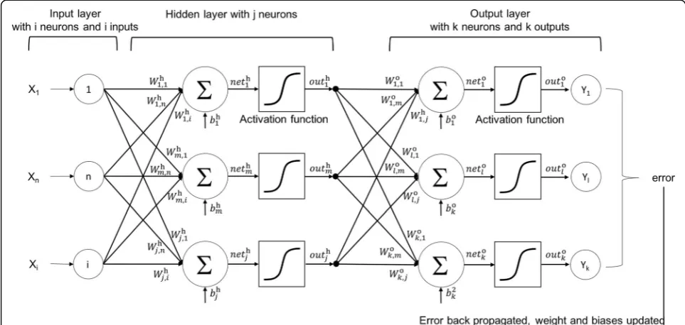
system. The ANN method offers a variety of network ar-chitectures suitable to different fields of application. In this study, we adopted the architecture most widely im-plemented in the climatology field: the feed-forward arti-ficial neural network (FFANN) (Abhishek et al.2012), a multi-layer perceptron trained using the back-propagation learning algorithm (MLP-BP). We used the FFANN for downscaling WRF rainfall output from D1 to D2. Figure3depicts the simplified architecture of the MLP-BP network implemented in this study. The net-work contains a set of neurons organized in layers from the input layer on the left to the output layer on the right. All the processing neurons are fully connected with other neurons in the following layer, while there is no connection between neurons of the same layer. The input layer is designed neither for processing data nor generating inputs of its own. It simply stores the input values to be processed in the next layer. After the input layer, one or more processing layers, called hidden layers, follow. The last layer is the output layer, contain-ing processcontain-ing neurons to generate a simulated value. The connections between neurons are made with the as-sociated weights. The network illustrated in Fig.3 repre-sents a three-layered ANN with an input layer ofiinput neurons (X1, X2,…, Xi), one hidden layer withjneurons (H1, H2, …, Hj), and k output neurons (Yz1, Y2, …,Yk), with connections from the output of one layer to the input of the next layer. The superscriptshandoindicate that the calculations are implemented in the hidden layer or output layer, respectively. The input values cal-culated by the model for them-th neuron in the hidden
layer are the weighted sum of iinputs to which the bias valuebhmis added:
nethm¼Xin¼
1W
h
m;nXnþbhm ;m¼1;2;…j ð5Þ
whereWhm;n is the associated weight matrix for the con-nection between the input neurons and the neurons in the hidden layer. Then, the nethm vector is entered into a non-linear activation function g(), which is essential for an ANN model to solve nonlinear problems. The most useful and widely adopted functions for g() are the hyperbolic tangent or logistic sigmoid (Bodri and Čer-mák 2001). In this study, the logistic sigmoid function was used first, and its simulation results were compared step-by-step with those produced using the hyperbolic tangent function. The output of neuron outhm in the hid-den layer subsequently becomes:
outhm¼g net hm ð6Þ
The input of thel-th neuron in the output layer is cal-culated as the weighted sum of those activations plus the bias neuronsbol:
netol ¼Xmj¼
1W
o
lmouthmþbol ;l¼1;2;…k: ð7Þ
The same activation function g() that was applied to the hidden layer is applied to the input layer. The final network output outol for thel-th output of the model is subsequently obtained using the following function:
outol ¼gnetol: ð8Þ
As the goal of training is to minimize the difference between the actual (desired) and simulated outputs, the network error is computed at this stage. This error is subsequently inserted back into the input layer, where the initial connecting weights and biases are adjusted according to the magnitude of the error. The supervised learning is repeated until the ANN converges to an error smaller than the threshold. In this study, the connection weights were updated after each training itinerary. ANN was trained using the Levenberg Marquardt training algorithm, which has been proven a fast and efficient update rule for medium-sized FFANN (Yu and Wila-mowski2011).
ANN downscaling experiment
The goal of an optimal ANN architecture is to minimize error between simulated output and the desired value with the most compact and simple structure possible. There are several essential factors affecting the performance of ANN, including the (1) predictor selection, (2) number of layers and neuron structure (network structure), and (3)
specified training algorithm for connecting weights. Input predictors are usually independent variables, believed to have some predictive power over the dependent variable (predictand). Normally, useful predictors could be selected by looking at correlations and cross-correlations between the predictors and predictand. However, the combination of two or more uncorrelated predictors might potentially become a strongly correlated variable (Castellano and Fanelli 2000). In contrast, two or more highly correlated predictors might exacerbate a small change in the model, potentially increasing the error. With regard to the net-work structure issue, while an insufficient number of hid-den neurons might lead to low accuracy in training, an excessive number of hidden neurons tends to add un-necessary training time, with marginal improvement or memorizing instead of learning (overfitting; Castellano and Fanelli2000). There is no specific method to find the optimal number of layers and hidden neurons, except for the commonly used trial and error approach (Zhang and Goh2016). On the last issue related to the training algo-rithm is that there are several training functions available to obtain the connection weights, as well as to adjust the weights. Training algorithm selection is made based on the type of network, input data, and occasionally, com-puter power.
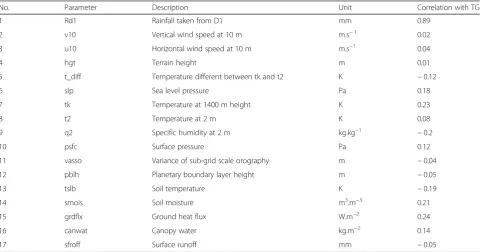
The predictors considered in this study are described in Table 2, along with their correlation coefficients with RD2T. Predictor variables were subsequently selected and tested using the trial-and-error method, from a
simple network of several correlated variables to the lar-ger sets, including the combination of uncorrelated vari-ables. To increase the efficiency of the training process, all selected variables were normalized using the feature
Fig. 4Predictor and predictand grid selection principles
Table 2Predictor variables considered in the preliminary test
No. Parameter Description Unit Correlation with TG
1 Rd1 Rainfall taken from D1 mm 0.89
2 v10 Vertical wind speed at 10 m m.s−1 0.02
3 u10 Horizontal wind speed at 10 m m.s−1 0.04
4 hgt Terrain height m 0.01
5 t_diff Temperature different between tk and t2 K −0.12
6 slp Sea level pressure Pa 0.18
7 tk Temperature at 1400 m height K 0.23
8 t2 Temperature at 2 m K 0.08
9 q2 Specific humidity at 2 m kg.kg−1 −0.2
10 psfc Surface pressure Pa 0.12
11 vasso Variance of sub-grid scale orography m −0.04
12 pblh Planetary boundary layer height m −0.05
13 tslb Soil temperature K −0.19
14 smois Soil moisture m3.m−3 0.21
15 grdflx Ground heat flux W.m−2 0.24
16 canwat Canopy water kg.m−2 0.14
scaling method described in Eq. 9 to transform all values into the range [0:1], where a(g)is the original value be-fore normalization occurs andzgis the normalized value of a(g). The reason for normalization is to avoid a very high resultant value when the original data is entered into the ANN, which could potentially cause the activa-tion funcactiva-tion to exhibit low performance in resolving small changes in the input data, thus losing sensitivity.
zg ¼ a gð Þ−minð Þa
maxð Þ−a minð Þa ;where a¼ða1;…;anÞ: ð9Þ
In the next step, the number of hidden layers and neu-rons were determined according to the quantity of vari-ables, gradually increasing the network size from a small neuron number until the desired accuracy was obtained. A common method for ANN training is to separate data into independent training and testing sets. However, it has been shown that better-trained models are not ne-cessarily associated with better estimation capability. An excessively complex network with a high parameter-to-observation ratio might lead to overfitting; that is, a model with very low predictive power even when it was well trained. A practical way to avoid overfitting while simultaneously improving the estimation capability of the network is to create a small set of data from the training set for cross-validation. The errors in the
training set and validation set are compared during the training stage. If error in the validation set continues to increase, the training process will be stopped, thus achieving the best network performance. We adopted the cross-validation approach to train the ANN model in this study. The data used in the training stage was randomized to avoid bias, subsequently being divided into 3 independent datasets: 75% of the data was set as the training set, 15% as the testing set, and the remaining 10% was set aside for cross-validation. During the preliminary stage, numerous ANN models were tested to find the most effective network design for rain-fall downscaling. In this section, several distinctive models, whose structures were considered the most suit-able for trial-and-error tests, are presented, with the model details summarized in Table3.
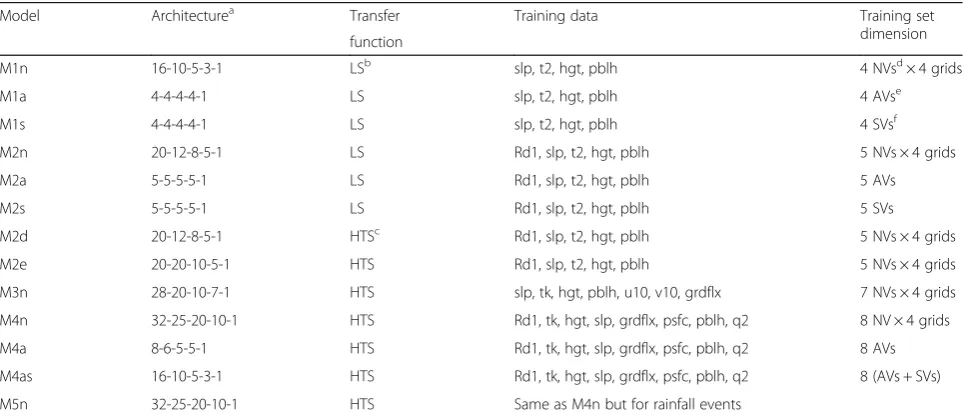
ANN structures can be modified in various ways to bring the best fit for the prediction model. Any adjust-ments in the three factors of ANN architecture, transfer function, and predictand quantity/type greatly affect net-work performance. In this research, the processing methods for each predictand were considered as a fourth major factor in model selection. The selected predictands for ANN training were treated in different ways then clas-sified into three types: normal variables (NV) were those extracted directly from the CTL result, while predictand average values (AV) and standard deviation values (SV) were taken for the four-predictor grid cells. Table 3 lists
Table 3Distinctive ANN models considered in the preliminary test
Model Architecturea Transfer Training data Training set
dimension function
M1n 16-10-5-3-1 LSb slp, t2, hgt, pblh 4 NVsd× 4 grids
M1a 4-4-4-4-1 LS slp, t2, hgt, pblh 4 AVse
M1s 4-4-4-4-1 LS slp, t2, hgt, pblh 4 SVsf
M2n 20-12-8-5-1 LS Rd1, slp, t2, hgt, pblh 5 NVs × 4 grids
M2a 5-5-5-5-1 LS Rd1, slp, t2, hgt, pblh 5 AVs
M2s 5-5-5-5-1 LS Rd1, slp, t2, hgt, pblh 5 SVs
M2d 20-12-8-5-1 HTSc
Rd1, slp, t2, hgt, pblh 5 NVs × 4 grids
M2e 20-20-10-5-1 HTS Rd1, slp, t2, hgt, pblh 5 NVs × 4 grids
M3n 28-20-10-7-1 HTS slp, tk, hgt, pblh, u10, v10, grdflx 7 NVs × 4 grids
M4n 32-25-20-10-1 HTS Rd1, tk, hgt, slp, grdflx, psfc, pblh, q2 8 NV × 4 grids
M4a 8-6-5-5-1 HTS Rd1, tk, hgt, slp, grdflx, psfc, pblh, q2 8 AVs
M4as 16-10-5-3-1 HTS Rd1, tk, hgt, slp, grdflx, psfc, pblh, q2 8 (AVs + SVs)
M5n 32-25-20-10-1 HTS Same as M4n but for rainfall events
a
Model architecture indicates the number of neuron in each layer of a 5-layer MLP network, wherein first number is neurons of input, the following three numbers are neurons of hidden layers, and the last one is neurons of the output layer
b
LSlogistic sigmoid
c
HTShyperbolic tangent sigmoid
d,e,f
NV,AV, andSVcorrespond to normal variable, averaged variable, and standard deviation variable, respectively; in which: -NVs are directly extracted from the 4-predictor grids, so the actual number of variable are multiplied to 4;
-AVs are the new features created by computing the mean of each variable in the 4-predictor grids;
13 ANN models in 5 groups with different adjustments based on the four criteria mentioned above. The M1 model series includes the simplest MPL network design, with a logistic sigmoid (LS) transfer function and four pre-dictor variables. The M2 model series aimed to further test the network by increasing the number of predictor variables to five and adopted both LS and hyperbolic tan-gent sigmoid (HTS) functions. The M3n and M4 model series focused on examining the importance of predictor factors by changing the combination of variables as well as increasing the number of variables. In all models, the MLP structure was adjusted with respect to the network size adjustment. The M5n models used the same setup as the M4n, but were trained for rainfall events (RE) only. In line with the DDE criteria, daily precipitation larger than 0.5 mm were considered RE events.
ANN models developed using the 1996–1998 datasets were applied to the WRF output for 2006. The aim of this application was to study the stability and applicabil-ity of WRF coupled with ANN for rainfall downscaling. Since the testing stage targets model reproducibility for any weather condition, the model that was designed to train with rainfall events only (RE-ANN, i.e., the M5n model) was expected to experience difficulty in reprodu-cing DDE cases. Therefore, its simulation output was calibrated to minimize bias. We tested the correlation of DDE cases in both D2T and D1, finding a very strong connection between DDE cells at the high-resolution scale with the DDE cells at the coarse scale. Spatially, 99. 44% of the DDE cells in D2T were located completely inside DDE cells in D1. Additionally, any cell in D2T partly overlapping with a DDE cell in D1 also had a 98. 27% chance of being labeled as a DDE cell. This result demonstrates that any cell in D1 has a significant simi-larity in rainfall condition to the child cells within and around it. Therefore, any cell in the RE-ANN model out-put with a spatial connection to a DDE cell in D1 was treated as a DDE. This treatment process for DDE cells in the model output was called the RE-ANN calibration and was also applied to the M5n model during the pre-liminary test.
Results and discussion
Dynamical downscaling experiment
This section evaluates WRF’s ability to reproduce weather conditions in D2T. Table 4 shows evaluation statistics for the spatial distribution of mean rainfall from CTL for D1 and D2 as compared with observed rainfall at 38 rain gauges in 1996, 1997, 1998, and 2006, along with the statis-tical measures R and IOA. According to Table 4, the JJA rainfall in CTL was noticeably underestimated in both D1 and D2, as illustrated in the average accumulated values of 784 mm in D1 and 799 mm in D2, versus 1107 mm in the observation data. Furthermore, the rainfall projections at all observation locations were lower than the observed values. The summarized statistic indicated that simulated rainfall in D2 was slightly closer to the observation data than it was in D1. Both spatial correlation and IOA between observa-tion data and CTL results exhibited slightly better values in D2 than in D1. This finding indicates that, in addition to the spatial resolution advantages, D2 can better resolve the finer resolution than can the D1. In D2, the ratio of the pre-cipitation average for D2T between CTL and the observed value was consistently lower than 1, ranging from 0.65 to 0. 82, with an average of 0.72. Both spatial correlation and IOA between D2 and the observations were relatively high, from 0.66 to 0.77 and 0.71 to 0.78, respectively. This indi-cates reasonable accuracy for the CTL in reproducing the spatial distribution of JJA rainfall. Regarding the underesti-mated rainfall in the CTL output, several studies (Bukovsky and Karoly2011; DeMott et al.2007) have experienced the same problem. A common insufficiency of climate models is that they often underestimate extreme precipitation events, while overestimating the occurrence of light precipi-tation events. In this study, we focused on the rainfall sea-son of a tropical country, where intense rainfall is a regular occurrence. Thus, it is not surprising to find that rainfall is underestimated in our simulation.
In addition to the spatial distribution of JJA accumu-lated rainfall, the temporal variations of daily rainfall be-tween CTL and observations for D2 were examined at 38 locations using the metrics of temporal R, MAE, and RMSE (Table 5). The CTL results for JJA during the
Table 4Statistical measures for WRF simulated rainfall over JJA periods
Year Mean
Obs (mm)
D1 D2
Mean CTLa(mm) CTL/Obs R IOA Mean CTL (mm) CTL/Obs R IOA
1996 1078 679 0.63 0.77 0.65 701 0.65 0.78 0.66
1997 983 764 0.75 0.73 0.75 772 0.78 0.74 0.77
1998 1167 903 0.77 0.71 0.75 893 0.77 0.71 0.74
2006 1198 974 0.81 0.71 0.7 983 0.82 0.71 0.7
Average 1107 784 0.74 0.73 0.71 799 0.76 0.74 0.72
a
Mean CTL was calculated by averaging the simulated rainfall from 38 location in CTL corresponding to the locations of rain gauges
IOAindex of agreement,Obsobservation
research period suggest a moderate temporal agreement with observations, in which the average correlation coeffi-cient for all 38 locations was 0.63. However, there was substantial variation in the correlation coefficients across the study site. While the temporal correlations for daily rainfall in midland and lowland areas, i.e., the Red River Delta, were high (average 0.7), the CTL output for the high mountainous regions was in low temporal agreement with the observations (average 0.5), especially in the areas between alternating high mountain ranges (as in the west-ern part of D2T, see Fig. 1c). This finding highlights the limitation of WRF in resolving micro-climatological con-ditions and covering complex topography effectively. The same conclusion was arrived at by Li et al. (2016) in their research on the influence of topography on precipitation distribution.
The average MAE for the testing locations was 4. 67 mm, while the average RMSE was significantly higher at 14.53 mm. Since the RMSE tends to amplify large biases, the large gap between the two values reflected the underestimation of heavy and extreme rainfall cases in the CTL, which partly resulted in underestimation of the accumulated rainfall mentioned above. The average correlation coefficient for all 38 locations indicates a moderate agreement, but there was large variation in correlation coefficients between the locations (detail not shown). JJA accounts for over 70% of the annual rainfall, which begins in June, peaks in late July, and decreases through August. The correlation coefficient results indi-cate that the proposed WRF setup can reproduce sea-sonal variation in rainfall relatively well, especially for the lowland region where D2T is located.
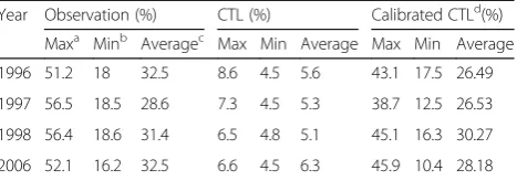
To examine the significance of the calibration method for DDE (omitting values less than 0.5 mm per day), we directly compared DDE during the JJA period from the CTL results, CTL calibrated results, and observed values for each observation location. The maximum, minimum, and average DDE percentages in D2T at the 38 locations are presented in Table6. The summarized results clearly show miscalculation of DDE by CTL. The percentage of DDE in the CTL results ranged from 4.5 to 8.6% of the total grid cells in D2, which were 4 to 6 times lower than the actual data across all years. The application of a wet
day threshold showed a good result in eliminating the biases between simulated and observed data, with a large improvement in the calibrated CTL results. Even when the ranges of maximum and minimum percentage DDE did not perfectly match the observations, the average DDE results for JJA in the calibrated CTL were very close to the observed average. However, quantitative as-sessment of the reduction in total rainfall owing to DDE calibration indicates that the mean total rainfall decrease is 0.28% for D1 (detailed result not shown here). Thus, the calibration helps WRF better capture DDEs, with a negligible effect on total rainfall. WRF simulation results for D2T after calibration were expected to be a good predictand for the ANN training stage.
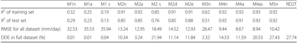
Results of the ANN preliminary training stage
This section describes the training stage results of rain-fall downscaling, using the MLP-based ANN on different model configurations as mentioned in Table3. To com-pare the predicted model outputs with the desired out-put, various statistical measurements were adopted. Their results are presented in Table 7, while regression plots for the testing set are shown in Fig. 5. Results of the training stage show substantial variations in perform-ance among the models. The training results improved with regard to higher model complexity; however, there was clear consistency in network performance, with most models exhibiting similar correlation coefficients in the training and test sets. The cross-validation method was proven to be effective in detecting the best generalization point and stopping the training process before the model shifted to over-learning.
The simplest designs in the M1 model series provided the worst results (very low accuracy and large RMSE) and were unable to forecast DDE cases. Figure5indicates that the M1n, M1a, and M1 s models heavily underestimated RD2T, which might be attributed to the low predictive power of the combination of variables sea level pressure (slp), temperature at 2 m (t2), geographical height (hgt), and planetary boundary layer height (pblh). However, the R2
coefficient indexes suggest that M1n was a better
Table 5Temporal correlation, RMSE, and MAE between CTL and Observation daily rainfall averaged for 38 locations for the JJA period in 1996, 1997, 1998, and 2006
D2 RRD NMR
Number of rain gauge 38 12 14
R 0.63 0.7 0.5
RMSE (mm) 14.53 9.12 17.98
MAE (mm) 4.67 3.52 7.21
RRDRed River Delta,NMRnorthern mountainous regions
Table 6Comparison of the percentage of DDE in JJA among 38 rain gauge locations
Year Observation (%) CTL (%) Calibrated CTLd(%)
Maxa Minb Averagec Max Min Average Max Min Average
1996 51.2 18 32.5 8.6 4.5 5.6 43.1 17.5 26.49
1997 56.5 18.5 28.6 7.3 4.5 5.3 38.7 12.5 26.53
1998 56.4 18.6 31.4 6.5 4.8 5.1 45.1 16.3 30.27
2006 52.1 16.2 32.5 6.6 4.5 6.3 45.9 10.4 28.18
a, b, c
Max,min, andaveragecorrespond to the maximum, the minimum, and the averages of DDE cases during JJA among 38 rain gauge
locations, respectively
d
Table 7RMSE andR2for training and test sets of different ANN model configurations
M1n M1a M1 s M2n M2a M2 s M2d M2e M3n M4n M4a M4as M5n RD2T R2
of training set 0.32 0.25 0.19 0.91 0.92 0.85 0.91 0.91 0.62 0.92 0.92 0.93 0.92 R2
of test set 0.29 0.23 0.13 0.85 0.85 0.76 0.85 0.88 0.51 0.92 0.91 0.92 0.92
RMSE for all dataset (mm/day) 32.53 35.53 35.94 13.24 12.95 18.49 14.52 12.93 28.47 9.44 8.67 8.94 10.42
DDE in full dataset (%) 0.01 0.01 0.04 10.34 3.24 21.94 11.14 11.84 2.32 14.53 11.59 20.53 27.43 27.74
model than M1a and M1s. While the M1n setting used the NV input features, which might be better than AV and SV, the accuracy levels of the M1 model series were too low to determine any differences. The M2 model series showed significantly better fitting and bias results compared to the M1 series. Except for M2s, with R2 for the test data of 0.76, the other M2 models yielded at least 0.85 for R2in the test set. The large improvement in the M2 series was achieved by incorporating the rainfall in D1 (RD1), which is highly correlated to RD2T (Table2). The sudden drop in the predictive power of the M3n model also indicates the significance of RD1 in model design, since M3n eliminated the RD1 variable in the training stage. With the same settings, the M2n and M2a models showed significantly better correlation to RD2T than did M2 s, thus indicating a lack of signal strength in SV features. Although M2s appears to be weaker, its simulated DDE percentage was 21.94%, which was close to that of RD2T (27.74%). The ability of M2s to resolve DDE was significantly better than those of M2n and M2a, whose DDE percentages were 10.34 and 3.24%, respectively. The reduction of DDE percentage in M2a reflected the drawback of the AV features, compared to the NV features, since the average value reduces the variation signal in the predictors. On the other hand, M2d and M2e exhibited slightly better results than did M2n, especially with regard to the reproducibility in DDE cases (11.14 and 11.84%). The large number of neurons and the high rescaling range—[−1:1] of HTS to [0:1] of LS—made it more convenient for the network to detect very small rainfall values.
The M4 series and M5n were clearly better than the other models, as their predictions were close to that of RD2T, yielding significantly lower RMSE. Add-ing more predictor variables have proven to be help-ful in increasing model accuracy. There was variation in the behaviors between the models in the M4 series, despite their skillful results. Even though the RMSE of M4a was lowest at 8.67 mm/day, its ability to map small rainfall signals was significantly lower than those of M4n and M4as. M4a indicated 11.59% DDE, while M4n and M4as indicated 14.53% and 20.53%, respectively. Compared to the DDE percentage of 27. 74% in RD2T, M4as was clearly the best at forecast-ing small rainfall values. The study results indicate that a combination of AV and SV features might be
better in detecting DDE. The higher RMSE values in M4n and M2n, as compared to the other M2 models, might be attributed to the interaction of highly correlated inputs among the NV features. The same behavior was also demonstrated by Wendemuth et al. (1993), who found that the combination of correlated inputs poten-tially adds more weight not only to the predictive informa-tion, but also to the biases. M5n discarded rainfall event information during the training stage, which understand-ably resulted in higher RMSE than the M4 model series. The RE-ANN calibration method was employed for the M5 model to successfully map a total of 27.43% DDE grid cells, which was smaller than that of RD2T by a small margin.
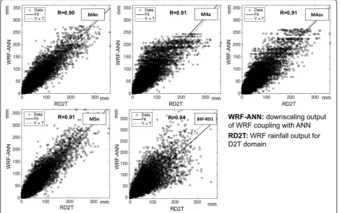
Results of WRF-ANN downscaling for an independent dataset
The second testing stage in this study aimed to further as-sess the applicability of coupling ANN to WRF output for high-resolution rainfall downscaling and compare it with the interpolated data using a bilinear interpolation method. We selected the ANN architectures that demonstrated the most promising global approximation abilities during the training stage (the M4 model series and M5n) to apply for an independent dataset for the year 2006. In addition, we also used bilinear interpolation to downscale RD1T from 30 to 6 km (denoted BIP-RD1). The summarized results of the tests are presented in Table8, while regression plots for the target and forecast rainfall are plotted in Fig.6. All models in the second stage continued to show predictive consistency in performance with the 2006 dataset (Table7). Differences in correlation coefficient metrics were observed, although they were in-significant. The correlation coefficients (> .9) for simula-tion outputs in this stage were comparable to results from the preliminary stage, indicating good model reproducibil-ity. However, in the 2006 dataset, the simulation results also exhibited more prediction errors, as can be seen in the RMSE. The unexpected reduction in model stability may be due to imperfect model design or a lack of repre-sentative information in the training dataset (Sánchez Lasheras et al.2010). Sometimes, the incomplete nature of model development may also contribute to the problem (Tu1996). The models that adopted NV variables, includ-ing M4n and M5n, were observed to have higher biases than those that adopted AV and SV variables, including
Table 8The second stage testing results of ANN models
M4n M4a M4as M5n BIP-RD1 2006-RD2Ta
Spatial correlation for 2006 dataset 0.9 0.91 0.91 0.91 0.84
RMSE for 2006 dataset (mm/day) 14.21 11.27 10.24 12.42 16.93
DDE in 2006 dataset (%) 9.54 15.94 19.48 23.84 17.43 23.78
a
M4a and M4as. Highly correlated NV inputs seemed to yield more error than their generalized features. Both M4a and M4as proved better than M4n at predicting the DDE percentage, with 15.94 and 19.48%, respectively, compared to 9.54%. Between the two, the M4as model, which inher-ited the predictive power of both SV and AV features, out-performed M4a in every measure. However, M5n is the model that delivered the best forecast of DDE percentage, at 23.84%, which was within 0.1% of the 2006-RD2T of 23. 78%. Since M5n was designed with the same setting as M4n, the RE-ANN calibration method was proven effect-ive in locating DDE cases. Results of the bilinear interpolation method, BIP-RD1, on the other hand, showed noticeably lower spatial correlation coefficients and higher RMSE values than did the ANN downscaling. DDE percentage determined by BIP-RD1 was 17%, much lower than the observed value of 24% in 2006-RD2T. The bilinear interpolation method generates estimated values between grid points. It is a simple and fast method, but lacks important embedded dynamical processes that are contained in the WRF models. The ANN method, on the other hand, performs downscaling by creating statistical relationships between high- and intermediate-resolution WRF outputs. ANN incorporates the dynamical processes given by WRF during the training processes. This added value provided by ANN helped to capture fine-scale
variations in the downscaling results. It is therefore rea-sonable to find that downscaling with ANN outperformed the bilinear interpolation method.
Comparisons between the ANN models and target data with regard to the frequency of dry days, wet days, and extreme rainfall events is shown in Fig. 7. The rain-fall frequency illustrated by all models was similar to that of RD2T, wherein the dry day and low rainfall (less than 20 mm) cases accounted for most of the days dur-ing JJA. Regarddur-ing the distribution of very low rainfall cases (less than 5 mm) and extreme rainfall cases (higher than 100 mm), the M4n and M4a models showed weak-ness in their underestimation of low rainfall cases. These two models failed not only in resolving the DDE cases as illustrated in Table8, but also in projecting small rainfall values. BIP-RD1 exhibited better DDE percentages than did the M4n and M4a models, but these were still much lower than the observed values. Meanwhile, the M4as and M5n were nearly identical, with rainfall frequencies in these two models being similar to the observed values. Both M4as and M5n showed significant improvement over M4n and M4a in locating small rainfall ranges.
The distribution maps for cumulative JJA rainfall in 2006 by M4n, M4a, M4as, M5n, and BIP-RD1 are depicted in Fig.8, in comparison with RD2T (2006-RD2T) and RD1 (2006-RD1). Owing to the high correlation with
2006-RD2T (Table8), ANN downscaled the rainfall in all models, clearly demonstrating a good pattern-correlation. The highest rainfall areas were accurately located in the southwestern corner of D2T, and rainfall gradually de-creased towards the northeast. While the spatial correla-tions of cumulative rainfall were similar among the models, the rainfall distribution results indicate an abso-lute strength of NV input features over AV and SV features, as pertains to the downscaled detail. We can explicitly recognize the smoother transition of rainfall withdrawal from higher to lower rainfall areas in the M4n and M5n models than is demonstrated in the M4a and M4as models. Compared to the 2006-RD2T distribution pattern, the rainfall transition patterns in M4n and M5n showed a loss in detail; even so, its resolution was suffi-ciently high to distinguish minor changes. The essence of the WRF-ANN downscaling method was the use of four D1 grid cells to predict one spatially overlapped grid cell in D2. When the resolution of D2 was too high for com-parison with D1, it was unavoidable that some adjacent cells in D2 would have the same predictor values. This problem results in predicted values repeating for some cells. Less detail was expected in M4n and M5n than in 2006-RD2T, since increasing resolution from 30 to 6 km is a large jump. As expected, both the M4n and M5n models showed significantly higher resolution than that of the 2006-RD1. In contrast, M4a and M4as had signifi-cantly lower resolution and coarse rainfall patterns. The differences between M4a and M4as were too small to
indicate any advantages from combining both AV and SV features for prediction. Even with their higher resolution, neither M4a nor M4as demonstrated better changes in the minor rainfall pattern. In this test, simulation results suggest that generalized features might be more effective in bias control. However, this approach loses essential in-formation for examining the spatial distribution of pre-cipitation, which leads to similar generalized results. On the other hand, while the original NV predictor exhibited a larger bias, it better mapped the variability in rainfall. BIP-RD1 showed larger increase in spatial resolution than did RD1T, but failed to generate the wide range of rainfall variation present in RD2T. It tended to overestimate rain-fall in light rainrain-fall grid cells and underestimate rainrain-fall in heavy rainfall grid cells.
The differences between cumulative JJA rainfall simulated by M4n, M4a, M4as, M5n, and BIP-RD1with RD2T are in-dicated in Fig.9. All models exhibited larger estimation er-rors in the northwestern part of D2T, especially in the high terrain and surrounding area. However, these large errors were not a surprise because this area accounts for the high-est JJA rainfall (Fig.8). The BIP-RD1 model showed slightly larger error than did the other models, while both M5n and M4n overestimated the total JJA cumulative rainfall, with M4n having the larger overestimation, as reflected in its RMSE. Since M5n neglected very small rainfall values dur-ing calibration, it potentially avoided bias intensification by small rainfall values during training. Moreover, in a com-parative study on software estimation efforts, Nassif et al.
(2012) also found an overestimation tendency by MLP-ANN, especially for an MLP trained with a complicated range of inputs. The model behavior suggests that small rainfall values, which accounted for 10 to 40% of the data-set, were difficult to reproduce by ANN. However, they can be addressed using the RE-ANN calibration methods.
Predictor sensitivity analysis
To obtain a comprehensive view on the applicability of coupling WRF and ANN to downscaling, the influence of each input predictor on the output should be investigated. Normally, variables with a higher correlation to the pre-dictand are expected to be more helpful in forecasting. However, an unusual combination of correlated or uncor-related variables might also be useful. In this study, we considered 17 variables (Table 2), gradually fine-tuning their combination through the trial and error method. Al-though we could not cover all possible combinations, our best effort so far—as used in the M5n model—
demonstrated promising results. Sensitivity analysis was conducted for each variable input for the M5n model to examine their significance to the ANN outputs. The sensi-tivity analysis method used in this study was introduced by Hung et al. (2009), in which each input parameter in the M5n model was alternately removed from the ensem-ble, subsequently comparing the performance statistics with the original. Since the M5n model utilized eight variables, including RD1, atmospheric temperature at 1400 mm (tk), hgt, slp, ground heat flux (grdflx), surface pressure (psfc), pblh, and humidity at 2 m (q2), there were eight models included in the sensitivity test. The results of the sensitivity test are presented in Table9.
As can be seen in Table 9, RD1 has the largest impact on the predictand. Excluding RD1 substantially reduced network performance. Meanwhile, the model indicated the second largest impact by q2, while the third and fourth most important parameters were tk and slp, whose results were very similar to each other. Among the remaining
variables, grdflx differed from the others by a higher RMSE, achieving the fifth position. The remaining vari-ables pblh, psfc, and hgt were the least important, since the models trained without them were comparable to the original M5n model.
Apart from input variables, it is also important to con-sider sensitivity to the treatment methods used for the input variables, which classify the variables into NV, AV, and SV features. While NV features tend to yield more error, they can resolve the spatial variability of rainfall. Meanwhile, generalized features such as AV and SV can better control the bias in prediction values, but have lower effective resolution. NV features were concluded to be the best fit for making WRF-ANN models.
Computational cost
The expected results when adopting WRF-ANN over WRF include a comparable downscaling quality with re-duced computational load and time. Since the step of downscaling from 30- to 6-km resolution using ANN gives results instantly, the advantage of using
WRF-ANN methods was measured by comparing the time consumption needed by WRF to downscale rainfall to 30 or to 6 km. Our measured results indicate that WRF downscaling to 6-km resolution took 9.3 times longer than downscaling to 30-km resolution. Rainfall down-scaling using the WRF-ANN method can therefore save up to approximately 89% of the computational cost, as compared to downscaling using WRF alone.
Conclusions
The possibility of coupling WRF and ANN for high-resolution rainfall downscaling was investigated with a case study from the Red River Delta in Vietnam. The evaluation shows that the WRF modeling system can reproduce temporal variation in the JJA daily rainfall rea-sonably well, but underestimates the total precipitation. Owing to the higher precision of WRF, the region appears to have more drizzle, resulting in significantly fewer dry days than were observed. However, by implementing a wet day threshold of 0.5 mm, we were able to correct this issue.
Table 9Performance statistics for ANN sensitivity analysis for 1996–1998 dataset
M5n W/o Rd1 W/o tk W/o hgt W/o slp W/o grdflx W/o psfc W/o pblh W/o q2 R2
of training set 0.92 0.48 0.88 0.92 0.88 0.9 0.91 0.91 0.86
R2
of test set 0.92 0.47 0.87 0.91 0.86 0.89 0.89 0.88 0.85
RMSE for all dataset (mm/day) 10.42 24.52 15.29 10.82 15.24 13.48 11.37 10.98 17.43
W/owithout
The best performing ANN model, M5n, produced high-resolution rainfall patterns that are highly correlated with WRF (r =0.91) and have low RMSE (12 mm/day). High-resolution rainfall in each grid cell was downscaled by tak-ing the climatological variables from the four grid cells in the coarse domain. The M5n model was configured as an MLP-BG network with three hidden layers using the hyperbolic tangent sigmoid activation function. The opti-mal predictors for M5n were rainfall in D1 (RD1), atmos-pheric temperature at 1400 mm (tk), geographical height (hgt), sea level pressure (slp), ground heat flux (grdflx), surface pressure (psfc), planetary boundary layer height (pblh), and humidity at 2 m (q2). In addition to having high accuracy, applying WRF-ANN is also expected to re-duce computational costs. Running 30-km WRF and using ANN to downscale to 6 km is 89% less expensive than running nested 30- and 6-km WRF simulations. We de-veloped a calibration method (RE-ANN) to help ANN better capture dry days. This method treats a grid cell in D2T as dry if it was touching a dry grid cell in D1. This improved our simulation of dry days with ANN. The net-work trained for RE events and calibrated with the RE-ANN calibration method delivered the best prediction for our study area and period. Statistical relationships created by ANN can be used to directly downscale climate infor-mation from 30-km WRF output to a 6-km grid with rea-sonable accuracy. The application of ANN with WRF was effective for rapidly downscaling daily basic rainfall data in a season at low computational cost.
To further improve predictive skill of the WRF-ANN model, an additional analysis of the model biases will be required, e.g., sources of overestimated cumulative rainfall during JJA. Such analysis will require more detailed and extensive comparison of the various model configurations and predictor combinations in ANN. Using the coupling methods, we plan to extend the applicability of WRF-ANN to an ensemble of climate models, in which the principal components of the model ensemble can be con-sidered as inputs for ANN downscaling. This approach will potentially help facilitate the use of ensemble model prediction, without the need for excessive time and com-putational power. Additionally, we plan to experiment with even higher resolution (finer than 6 km) downscaling using WRF-ANN.
Abbreviations
AMSR:Microwave Instruments Advanced Microwave Scanning Radiometer; ANN: Artificial neural network; AVHRR: Advanced Very High Resolution Radiometer; BouLac: Bougeault and Lacarrere; DJF: December, January, February; FFANN: Feed-forward artificial neural network; GCMs: Multiple general circulation models; IOA: Index of agreement; JJA: Jun, July, August; JMA: Japan Meteorological Agency; JRA-55: Japanese 55-year reanalysis; MAE: Mean absolute error; MLP: Multi-layer perceptron; MLP-BP: Multi-layer perceptron trained using back-propagation learning algorithm; MM5: Fifth-generation mesoscale model; NCEP: National Center for Environmental Prediction; NCEP-FNL: NCEP Final Operational Global Analysis data; NCHMF: Vietnam National Centre for Hydro-meteorological Forecasting; NOAA OI SST: NOAA Optimum
Interpolated 1/4 Degree Daily Sea Surface Temperature Analysis; NOAA: National Oceanic and Atmospheric Administration; PSU/
NCAR: Pennsylvania State University/National Center for Atmospheric Research; RCM: Regional climate model; RMSE: Root mean square error; RRTM: Rapid radiative transfer model; SLP: Single layer perceptron; WRF: Weather research and forecasting
Acknowledgements
We thank the Vietnam National Centre for Hydro-Meteorological Forecasting (NCHMF), Japan Meteorological Agency (JMA), National Centers for Environ-mental Prediction (NCEP), and National Oceanic and Atmospheric Adminis-tration (NOAA) for producing and making their data output available. We would like to thank the anonymous reviewers whose suggestions helped to greatly improve the manuscript.
Funding
Not applicable.
Authors’contributions
QAT proposed the topic, conceived and carried out the simulations. KT collaborated with QAT, contributed to the design of the study, analyses, and interpretation of the results. Both QAT and KT drafted the manuscript. All authors read and approved the final manuscript.
Authors’information
QAT is a graduate student in the Department of Environmental Design, Kanazawa University graduate school of Natural Science and Technology. KT is an Assoc. Prof and Senior Researcher in the in the Department of Environmental Design, Kanazawa University graduate school of Natural Science and Technology.
Competing interests
The authors declare that they have no competing interest.
Publisher’s Note
Springer Nature remains neutral with regard to jurisdictional claims in published maps and institutional affiliations.
Author details 1
School of Natural Science and Engineering, Kanazawa University,
Kakuma-machi, Kanazawa 920-1192, Japan.2School of Environmental Design, Kanazawa University, Kakuma-machi, Kanazawa 920-1192, Japan.
Received: 10 November 2017 Accepted: 23 April 2018
References
Abhishek K, Singh MP, Ghosh S, Anand A (2012) Weather forecasting model using artificial neural network. Procedia Technology 4:311–318.https://doi. org/10.1016/j.protcy.2012.05.047
Berg N, Hall A, Sun F, Capps S, Walton D, Langenbrunner B, Neelin D (2015) Twenty-first-century precipitation changes over the Los Angeles region*. J Clim 28(2):401–421.https://doi.org/10.1175/jcli-d-14-00316.1
Bodri L,Čermák V (2001) Neural network prediction of monthly precipitation: application to summer flood occurrence in two regions of Central Europe. Stud Geophys Geod 45(2):155–167.https://doi.org/10.1023/a:1021864227759 Bougeault P, Lacarrere P (1989) Parameterization of orography-induced
turbulence in a mesobeta—scale model. Mon Weather Rev 117(8):1872– 1890.https://doi.org/10.1175/1520-0493(1989)117<1872:pooiti>2.0.co;2 Bukovsky MS, Karoly DJ (2011) A regional modeling study of climate change
impacts on warm-season precipitation in the Central United States*. J Clim 24(7):1985–2002.https://doi.org/10.1175/2010jcli3447.1
Caldwell P, Chin H-N S, Bader DC, Bala G (2009) Evaluation of a WRF dynamical downscaling simulation over California. Clim Chang 95(3–4):499–521.https:// doi.org/10.1007/s10584-009-9583-5
Castellano G, Fanelli AM (2000) Variable selection using neural-network models. Neurocomputing 31(1–4):1–13.https://doi.org/10.1016/S0925-2312(99)00146-0 Chen F, Dudhia J (2001) Coupling an advanced land surface–hydrology model
with the Penn State–NCAR MM5 modeling system. Part I: model
DeMott CA, Randall DA, Khairoutdinov M (2007) Convective precipitation variability as a tool for general circulation model analysis. J Clim 20(1):91–112. https://doi.org/10.1175/jcli3991.1
Dudhia J (1989) Numerical study of convection observed during the winter monsoon experiment using a mesoscale two-dimensional model. J Atmos Sci 46(20):3077–3107.https://doi.org/10.1175/1520-0469(1989)046<3077: nsocod>2.0.co;2
Fuentes U, Heimann D (2000) An improved statistical-dynamical downscaling scheme and its application to the alpine precipitation climatology. Theor Appl Climatol 65(3):119–135.https://doi.org/10.1007/s007040070038 Giorgi F, Mearns LO (1991) Approaches to the simulation of regional climate
change: a review. Rev Geophys 29(2):191–216.https://doi.org/10.1029/ 90RG02636
Guyennon N, Romano E, Portoghese I, Salerno F, Calmanti S, Petrangeli AB, Tartari G, Copetti D (2013) Benefits from using combined dynamical-statistical downscaling approaches – lessons from a case study in the Mediterranean region. Hydrol Earth Syst Sci 17(2):705–720.https://doi.org/10. 5194/hess-17-705-2013
Hong S-Y, Dudhia J, Chen S-H (2004) A revised approach to ice microphysical processes for the bulk parameterization of clouds and precipitation. Mon Weather Rev 132(1):103–120.
https://doi.org/10.1175/1520-0493(2004)132<0103:aratim>2.0.co;2
Hung NQ, Babel MS, Weesakul S, Tripathi NK (2009) An artificial neural network model for rainfall forecasting in Bangkok, Thailand. Hydrol Earth Syst Sci 13(8):1413–1425.https://doi.org/10.5194/hess-13-1413-2009
Kjellstrom E, Barring L, Nikulin G, Nilsson C, Persson G, Strandberg G (2016) Production and use of regional climate model projections - a Swedish perspective on building climate services. Clim Serv 2-3:15–29.https://doi.org/ 10.1016/j.cliser.2016.06.004
Kobayashi S, Ota Y, Harada Y, Ebita A, Moriya M, Onoda H, Onogi K, Kamahori H, Kobayashi C, Endo H, Miyaoka K, Takahashi K (2015) The JRA-55 reanalysis: general specifications and basic characteristics. Journal of the Meteorological Society of Japan. Ser II 93(1):5–48.https://doi.org/10.2151/jmsj.2015-001 Li Y, Lu G, Wu Z, He H, Shi J, Ma Y, Weng S (2016) Evaluation of optimized WRF
precipitation forecast over a complex topography region during flood season. Atmosphere 7(11):145
Mlawer EJ, Taubman SJ, Brown PD, Iacono MJ, Clough SA (1997) Radiative transfer for inhomogeneous atmospheres: RRTM, a validated correlated-k model for the longwave. Journal of Geophysical Research: Atmospheres 102(D14):16663–16682.https://doi.org/10.1029/97JD00237
Nassif AB, Capretz LF, Ho D (2012). Estimating software effort using an ANN model based on use case points. Paper presented at the 2012 11th International Conference on Machine Learning and Applications NCEP (2000). NCEP FNL operational model global tropospheric analyses,
continuing from July 1999 (publication no.https://doi.org/10.5065/ D6M043C6). From research data archive at the National Center for Atmospheric Research, Computational and Information Systems Laboratory Onogi K, Tsutsui J, Koide H, Sakamoto M, Kobayashi S, Hatsushika H, Matsumoto T, Yamazaki N, Kamahori H, Takahashi K, Kadokura S, Wada K, Kato K, Oyama R, Ose T, Mannoji N, Taira R (2007) The JRA-25 reanalysis. Journal of the Meteorological Society of Japan. Ser. II 85(3):369–432.https://doi.org/10.2151/ jmsj.85.369
Pierce DW, Das T, Cayan DR, Maurer EP, Miller NL, Bao Y, Kanamitsu M, Yoshimura K, Snyder Mark A, Sloan Lisa C, Franco G, Tyree M (2012) Probabilistic estimates of future changes in California temperature and precipitation using statistical and dynamical downscaling. Clim Dyn 40(3–4):839–856.https://doi. org/10.1007/s00382-012-1337-9
Reynolds RW, Smith TM, Liu C, Chelton DB, Casey KS, Schlax MG (2007) Daily high-resolution-blended analyses for sea surface temperature. J Clim 20(22): 5473–5496.https://doi.org/10.1175/2007jcli1824.1
Arritt, R. W, Rummukainen, M (2011). Challenges in regional-scale climate modeling. Bull Am Meteorol Soc, 92(3), 365–368. doi:https://doi.org/10.1175/ 2010bams2971.1
Salathé EP Jr, Steed R, Mass CF, Zahn PH (2008) A high-resolution climate model for the U.S. Pacific northwest: mesoscale feedbacks and local responses to climate change. J Clim 21:5708–5726.https://doi.org/10.1175/2008JCLI2090.1 Sánchez Lasheras F, Vilán Vilán J. A, García Nieto PJ, del Coz Díaz JJ (2010). The
use of design of experiments to improve a neural network model in order to predict the thickness of the chromium layer in a hard chromium plating process. Math Comput Model, 52(7–8), 1169–1176. doi:https://doi.org/10. 1016/j.mcm.2010.03.007
Seaby LP, Refsgaard JC, Sonnenborg TO, Stisen S, Christensen JH, Jensen KH (2013) Assessment of robustness and significance of climate change signals for an ensemble of distribution-based scaled climate projections. J Hydrol 486:479–493.https://doi.org/10.1016/j.jhydrol.2013.02.015
Skamarock WC, Klemp JB, Dudhia J, Gill DO, Barker DM, Huang XY, Wang W, Powers JG (2008). A description of the advanced research WRF version 3. Technical note, NCAR/TN-475 + STR
Storch HV, Langenberg H, Feser F (2000) A spectral nudging technique for dynamical downscaling purposes. Mon Weather Rev 128(10):3664–3673. https://doi.org/10.1175/1520-0493(2000)128<3664:asntfd>2.0.co;2 Tu JV (1996) Advantages and disadvantages of using artificial neural networks
versus logistic regression for predicting medical outcomes. J Clin Epidemiol 49(11):1225–1231.https://doi.org/10.1016/S0895-4356(96)00002-9 Walton DB, Hall A, Berg N, Schwartz M, Sun F (2017) Incorporating snow albedo
feedback into downscaled temperature and snow cover projections for California’s sierra Nevada. J Clim 30(4):1417–1438.https://doi.org/10.1175/ JCLI-D-16-0168.1
Walton DB, Sun F, Hall A, Capps S (2015) A hybrid dynamical–statistical downscaling technique. part I: development and validation of the technique. J Clim 28(12):4597–4617.https://doi.org/10.1175/jcli-d-14-00196.1
Wendemuth A, Opper M, Kinzel W (1993) The effect of correlations in neural networks. J Phys A Math Gen 26(13):3165
Yu H.,Wilamowski BM. (2011). Intelligent systems. In J. D. Irwin (Ed.), Intelligent Systems (pp. Pages 1–16): CRC Press