The attached paper represents an excursion into the area of dataflow computing and architectures. In the middle 1980s the ‘microprocessor revolution’ held out the possibility of developing new microprocessors with radically new architectures. This was also the era of the Japanese “Fifth Generation” computer architecture efforts and of the Alvey programme in the UK. Dataflow, it seemed, might provide a sympathetic architecture for executing highly parallel programs in a functional style. Unfortunately, all the dataflow machines of that era hit the buffers, because nobody was able to overcome the twin problems of designing a Matching Store that was fast enough and the sheer architectural challenge of bussing enabled instructions to available proces-sors. Indeed, Maurice Wilkes in his “Memoirs of a Computer Pioneer” (1985) says just how exciting the dataflow model would be if only someone could solve the architectural problems … (!)
This paper appeared in the journal “New Generation Computing” Vol. 3 No. 2 (OHMSHA/Springer-Verlag) in 1985. As far as I know this paper is not available online but a cover page and details of the journal are available via http://www.springer.com.
COLOPHON
The rebuild of this final draft started with scanning in to Omnipage OCR from a an original off-print. The recognition accuracy was surprisingly good. UNIX troff was used to set up the correct typeface (Times) and to get the line and page breaks as accurate as possible. Specialist material within the paper was re-set with the eqn , tbl and psfig pre-processors for troff .
The diagrams were also scanned in from the original offprint of the paper, cleaned up in Adobe Photoshop and then vectorized using Adobe Streamline. Further small adjustments were per-formed in Adobe Illustrator before exporting each diagram to version 3.2 of Illustrator’s Encapsu-lated PostScript (but with no TIFF preview). This EncapsuEncapsu-lated PostScript was then incorporated into the paper using psfig .
This form of “rescue” of an early paper can produce a very pleasing result but the time taken to do it (8 hours for this paper) makes it prohibitively expensive for any publisher to undertake as a general procedure, especially given that you need to be totally familiar with something like troff/eqn, or LATEX before you can even begin. The vast majority of the time taken for this paper
New Generation Computing, 3(1985) 181–195
The MUSE Machine — an Architecture for Structured
Data Flow Computation
David F. BRAILSFORD and R. James DUCKWORTH
Computer Science Group, University of Nottingham,
NOTTINGHAM NG7 2RD, England
Received 20 December 1984
Revised manuscript received 30 April 1985
Abstract
Computers employing some degree of data flow organisation are now well established as providing a possible vehicle for concurrent computation. Although data-driven computation frees the architecture from the constraints of the single program counter, processor and global memory, inherent in the classic von Neumann computer, there can still be problems with the unconstrained gen-eration of fresh result tokens if a pure data flow approach is adopted. The advan-tages of allowing serial processing for those parts of a program which are inherently serial, and of permitting a demand-driven, as well as data-driven, mode of operation are identified and described.The MUSE machine described here is a structured architecture supporting both serial and parallel processing which allows the abstract structure of a pro-gram to be mapped onto the machine in a logical way.
Keywords: Data Flow, Parallel Computation.
§1.
IntroductionIn recent years there have been many research projects investigating the design of novel architectures for the parallel evaluation of computer programs. Some of these have been motivated by the goal of achieving faster execution for all types of program; others have been fuelled by the goal of providing a more sympathetic environment for programs written in functional or logic languages. Such languages are notoriously slow in execution on conventional computers but their well-defined semantics and freedom from side-effects makes them ideally suited to parallel execution.
Backus in his ACM Turing award lecture,1) and his proselytism has been all the more effective considering that twenty years earlier he was the principal architect of a language2) whose very popularity has done much to preserve the traditional, or von Neumann, style of sequential computer architecture.
Although the virtues of a functional style are all too apparent we believe that most programmers trained in conventional languages will continue to expect con-structs such as loops and assignment statements. Languages such as SISAL 3) and Occam 4) show how conventional languages can evolve to permit parallel constructs without losing too many traditional features, Ideally new architectures should be capable of handling both the traditional and functional styles without undue language restrictions and without compromising too seriously the efficiency of execution.
The architecture of the MUSE (MUltiple Stream Evaluator) machine was designed from the outset to allow a tree or directed graph representing the struc-ture of a program, to be “flattened” onto a set of streams and for evaluation to take place, in parallel, on those streams. The MUSE machine has many features of data flow architecture but in its detailed operation it steers a middle course between a pure data flow machine,5) a tree machine6) and the graph reduction approach exemplified by ALICE.7) By mapping the program structure onto streams it is possible to relate the program text to the actual stream or streams which will execute each expression. In this way it is possible to obtain parallel execution while retaining conventional serial evaluation for those programs, or parts of a program, which are inherently sequential. Furthermore, the assignment of expressions to particular streams enables some degree of debugging to be undertaken should the machine become deadlocked or develop a fault.
§2.
Control of Computer Systems Supporting Concurrent ComputationThere are three types of control currently being investigated world-wide: control-driven, data-driven, and reduction (also known as demand-driven). Most computer systems being investigated incorporate one of these types of control and the rest are usually a hybrid of these. The MUSE machine has features typi-cal of both control-driven and data-driven systems, and is also capable of being programmed in a demand-driven fashion.
Reduction systems, or demand-driven systems, cause activity to be triggered by the demanding of results. These demands cause further demands for results and eventually, at some point, the demands find actual values rather than more sub-programs. These results are then combined operationally thus providing results which are the values required further on, this process eventually provid-ing the overall program result.
The difference between these two decentralised types of computation system may be summarised as follows: in a data-driven system all operations with avail-able operands are executed as soon as possible even if the results are not required. In a demand-driven system the processing elements only execute opera-tions as and when the results are required.
A comprehensive discussion on the relative advantages and disadvantages of data-driven and demand-driven computer architectures, and examples of each, is given by Treleaven, Brownbridge and Hopkins in Ref. 8).
§3.
Data Flow ComputationThis section gives only a brief introduction to data flow computation sufficient to illuminate the detailed description of MUSE operation which is covered in a later section. A review of various aspects of data flow computation is contained in Ref. 9).
Data flow computation is a fundamentally different way of carrying out instruction execution on computers. Instead of the program counter in the tradi-tional von Neumann model of computation determining the next instruction for execution, the presence of data for an instruction determines if that instruction may be executed. If many instructions have their operands available then these instructions may be executed concurrently assuming that sufficient resources are available.
The idea of data-driven computation stems from the work of Karp and Miller10) in the 1960s. Much of the early work on incorporating these ideas into machine architecture was carried out by Dennis at MIT.11) There are now many researchers working worldwide on data flow computers and a number of machines are operational in the US,12) Europe5) and Japan.13)
Programs to be run on a data flow machine are usually first translated into a data flow program graph which enables the data dependencies and potential parallelism in the program to be readily identified.
3.1.
Data Flow Program Graphsa
b
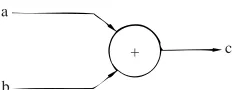
[image:5.594.179.296.63.108.2]+ c
Fig. 1 An example of a data flow program graph node.
Tokens are placed on and removed from the arcs of a program graph accord-ing to firaccord-ing rules. For the above node, it would be primed if there were tokens on the two input arcs and none on the output arc (in some literature the term “enabled” is used but we reserve this expression for the SEQUENCER operation in the MUSE — described in Section 5).
In most data flow computers a primed node may be executed or FIRED by a processing unit, but our multi-stream approach adds further firing con- straints which will be discussed later. A fired node consumes the input tokens and gen-erates a RESULT token on the output arc. The result token contains a data value which is the result of the function carried out on the input or source operands. The result token also contains a label which is an address pointing to the next node to which it must he sent.
Conditional operations may be performed by nodes which have a boolean control are as one of their inputs. In a conditional node the data input token is directed to either the true or false output are dependent on the condition of the boolean token on the control arc. An example of a conditional node is the “Branch” operator in Fig. 2.
Nodes may be connected together to form program graphs as shown in Fig. 3. Tokens bearing values for a and b and c at the three inputs will enable computa-tion of the expression
x =( a * b )+( b−c )
A token bearing the result value will be generated and output on arc x,
Another representation for data flow programs uses activity templates to
Data input
BR Control input
[image:5.594.272.406.475.600.2]T F
Fig. 2 An example of a conditional node.
a
b
c
x *
+
_
[image:5.594.92.199.481.580.2]represent the nodes of the data flow program graph.14)
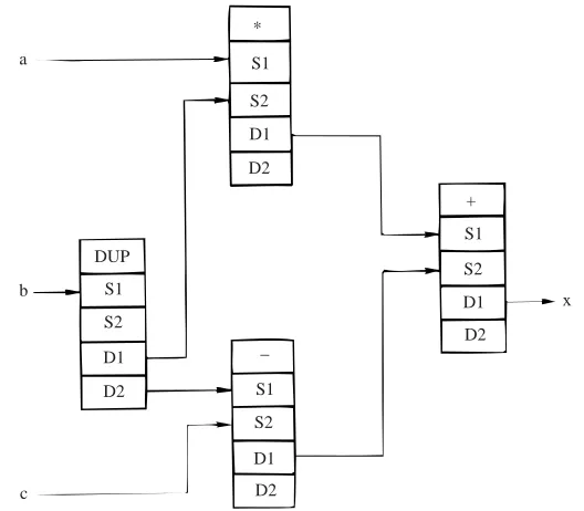
A configuration of activity templates for the same arithmetic expression is shown. in Fig. 4. It can be seen that there are five fields in each template: the first one contains the operation code specifying the operation to be performed, the next two fields hold the two source values or operands; and a further two fields contain the destination addresses for the result value. The provision of two desti-nation address fields allows result tokens to be sent to two separate destina- tions and it also allows conditional operations to be performed as described above. A result value may thus be sent to one or both destinations depending on the func-tion being performed. Whilst activity templates could have fewer or more fields, the above configuration of five fields allows any complex operation to be per-formed by combining one or more of these primitive templates. This configuration has formed the basis of the prototype MUSE machine.
The node description part of the activity template is fixed when the program is loaded and consists of the operation code field and the destination fields. The two source fields are the variable part of the template and whether they are filled or not influences whether the node can be executed. As explained earlier, if the two source value fields are filled then that node is primed.
Data flow has enormous potential for speeding up calculations, this has
a
b
c
*
S1
S2
D1
D2
DUP
S1
S2
D1
D2
_
S1
S2
D1
D2
+
S1
S2
D1
D2
[image:6.594.104.368.312.543.2]x
Fig. 4 An example showing how activity templates may be connected together. Notice the use of
been achieved by removing the program counter and global memory of the von Neumann machine. The physical connection between a von Neumann processor and its global memory has been called by John Backus “the von Neumann Bottleneck”.1) The data flow approach may have removed this bottleneck but it introduces the danger of removing all control and monitoring of a program’s exe-cution. If a data flow program works then all is well and good, but if it fails then there is often no easy mechanism for retrieving or isolating the fault.
The MUSE design allows code sequences which are intrinsically serial in nature to be allocated to streams in such a way that serial execution takes place naturally. Moreover the overall structure of the program can be mapped in a log-ical way onto the available streams as explained in the following section.
§4.
Evaluation on StreamsThe word “Stream” is used by a number of researchers in varying contexts e.g. streams in the language SISAL3) are sequences of values produced in order and Weng15) used the term in his recursive data flow schemas. Stream is used in the MUSE context to indicate a physical partitioning of the program among pro-cessing resources.
The word “Colour” is also used by a number of researchers and is usually used to differentiate data values which belong to separate invocations of some part of the program. In the MUSE the word colour is used to identify different blocks of program code.
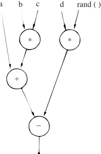
The operation of MUSE is best illustrated by taking a simple example. Con-sider the simple arithmetic expression:
a+b * c−d * rand( )
where a, b, c and d represent integers (say) and rand( ) is a function call to a random number generator which will eventually yield an integer. A data flow
a b c d rand ( )
* *
+
[image:7.594.80.180.436.589.2]_
Fig. 5 A data flow program graph of the
expression a−b * c−d * rand( )
Stream
No. Program Code
0 a ;↓1 ; + ;↓2 ; -1 b ; c ; * ;↑0 2 d ;↓3 ; * ;↑0 3 … “rand( )” …;↑2
. . .
n
[image:7.594.309.421.445.607.2]
Fig. 6 The graph of Fig. 5 mapped
graph of this expression is shown in Fig. 5 and one way of flattening that graph onto four streams is shown in Fig. 6. Note that the item “rand( )” on stream 3 is meant to indicate some suitable sequence of code to produce the required random number.
A processing agent is associated with each stream and the program code on each stream is evaluated serially, left to right. Each sub-expression is rep-resented in postfix notation and, for the sake of simplicity, we shall assume that operands such as a represent some integer literal which is instantly available. The interpretation of items such as↓1 (read as “down 1”) on stream 0 is “waiting for operand to arrive from stream 1”. Note that the sub-expression b*c is evaluated on stream 1 and communicates its result back to stream 0 by↑0 (read as “up 0”). Thus the up and down arrows act as a kind of labelled semaphore and, in the example we have just analysed, the↓1 on stream 0 is exactly matched by the ↑0 on stream 1. The function call of rand( ) we may presume to be evaluated on streams 3…n but its result is communicated back from stream 3, to the place where it is needed, by the↑2 command.
It will be obvious that, via a static trace starting at stream 0, we can write down each operand and operator as it is encountered and change stream as directed by the up and down arrows. In this way the postfix form of the original expression can be recovered and the integrity of code generation can be checked.
The code on each stream is executed sequentially with the proviso that it is necessary for each processing agent to suspend operation whenever it encoun-ters a down arrow or when it exhausts the sequence of code on its stream. This would imply that the processors spend much of their time idle and, to remove this problem, MUSE has an environment switching mechanism described in the next section.
4.1.
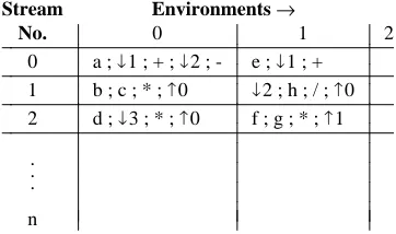
Environment SwitchingAssociated with each stream on the MUSE machine is an environment switching mechanism similar in some respects to the context switching on the Texas Instruments 9900 series of computers.16) A set of conventional program counters is kept for each environment on a given stream. Whenever computation is held up in any environment on any given stream, an automatic internal inter-rupt occurs, on that stream, to some other environment where computation can proceed. The different environments are labelled by a number in the range 0 – m and are also referred to by the alternative terminology colour 0 to colour m. By suitably arranging the interrupt priorities it is possible to impose a hierarchical interrupt system, wherein environment 0 has top priority, or to acquiesce in a more democratic round-robin scheme. Figure 7 Shows the allocation of the arith-metic expressions
Stream Environments→
No. 0 1 2
0 a ;↓1 ; + ;↓2 ; - e ;↓1 ; + 1 b ; c ; * ;↑0 ↓2 ; h ; / ;↑0 2 d ;↓3 ; * ;↑0 f ; g ; * ;↑1
. . .
n
[image:9.594.147.328.54.161.2]
Fig. 7 Mapping program segments onto different environments
The streams continue to operate asynchronously with respect to execution of code and changes of environment but the retention of a program counter and the allocation of code to specific streams enables some concept of machine state to be retained despite the fact that parallel evaluations are taking place.
4.2.
Compiler StrategyIt will be readily apparent from Fig. 7 that a compiler which produces code for the MUSE machine has a wide choice of strategies for distributing code among streams and colours. The starting point for the compiler’s deliberations is the data flow program graph, which is very closely related to the tree structure of the program. Figure 5, for instance, can also represent a program tree, but the root of the tree (the “−” operator) appears at the bottom of the diagram rather than at the top. Starting from the root the compiler locates the longest path from the root to a leaf. Code for this main path can then be laid out on some chosen stream and environment. Subsequent processing in the compiler identifies all the shorter paths which branch off the main path, together with the positions at which those subsidiary paths join the rest of the structure.
Having identified the various paths the compiler then has a clear choice regarding code layout on the streams. In a highly "vertical" strategy the code fragments could be laid out on successive streams (up to the maximum number of streams available) but would make little or no use of the colours. Conversely a “horizontal” approach might use all the colours on any given stream before proceeding to the next stream.
Our current compiler for arithmetic expressions is set up so as to allow for various strategies, ranging from the fully vertical to the fully horizontal. In this way it can generate code which tests out the performance and timing aspects of the MUSE prototype relating to the parallel activity on the streams and the dynamic switching of environments.
§5.
The MUSE Architectureto a set of streams and for evaluation to take place, in parallel, on these streams. Although parallel computation is possible by executing instructions on a number of streams, the actual instruction execution within a stream is sequential. This enables those programs or parts of programs that are inherently sequential to be executed as such.
A block diagram showing the pipelined ring architecture of the MUSE is given in Fig. 8. The stream nature of the MUSE allows parallel activity to occur over the streams but concurrent activity within each stream is also possible a result of the pipelined stages.
Sequencer
Sequencer
Sequencer Program Store Program Store
Program Store
Matching Store
Processor Processor
Processor
Switch
out in Stream 0
Stream 1
[image:10.594.127.348.201.473.2]Stream n
Fig. 8 A block diagram of the MUSE
The Processor on each stream accepts a complete node description (with a format similar to the activity templates described earlier) and carries out the function described by the operation code. A result is generated which is passed through the Switch. The Switch handles input and output on the MUSE and the result token’s address is checked to see if it is destined for an output device, perhaps for display on the console. If the result token is to form the operand of another instruction then it is passed on to the Matching Store. This is a simple store using conventional co-ordinate addressable memory devices to match tokens destined for the same instruction but different operand fields. The Match-ing Store is similar to that used by Manchester University5) but because it does not support matching of labels or other fields it is far simpler in operation.
When both operands are available for a particular instruction the Matching Store sends them to the required stream. They are combined with the node description part of the instruction to form a “primed” instruction.
MUSE has many features of data flow architecture and it is a data-driven machine up to the point of priming the instructions for firing. However, to enforce the sequential operation of various parts of the program a SEQUENC-ER has been specially designed. This gives some measure of control flow to the machine and is similar to the program counter in the von Neumann model.
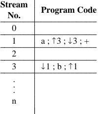
By contrast if it is desired to impose a demand-driven style of operation then the use of the↑ and↓ primitives can enforce this. Figure 9 shows a hypothetical sequence wherein the operand b required for the addition operation on stream 1 is actually produced on stream 3. The initial↓1 on stream 3 inhibits the value from being produced until the activation signal↑3 is executed on stream 1. Thus we see that the↑3,↓3 sequence on stream 1 is in effect asking stream 3 to produce the value and then waiting for it to appear. (This effect is achieved on the proto-type MUSE by passing a dummy data value between the ↑3 and ↓1 matching pair.)
Although the MUSE prototype has been closely modelled on the data flow description in Section 3 its main operational differences lies in the selection
Stream
No. Program Code
0
1 a ;↑3 ;↓3 ; + 2
3 ↓1 ; b ;↑1 .
. . n
[image:11.594.188.288.476.592.2]
Fig. 9 An example of code on two streams showing the operation of the up and down arrows in
mechanism for the next primed instruction to be executed. In most data flow computers, when an instruction becomes primed, it is sent immediately to a free processing unit for execution. In our approach we have added further constraints before an instruction can be executed.
5.1.
The SequencerAn important part of the MUSE operation is invested in the sequencer, there being one sequencer for each stream. Its function is to select the next instruction for execution, subject to a number of constraints. The overriding requirement is the presence of the instruction’s operands as in all data flow machines but this is no longer the only requirement that an instruction has to satisfy before it may be sent to a processor for execution. In the MUSE the instruction selected for exe-cution is dependent on the exeexe-cution of other related instructions. The use of the sequencer ensures that specific parts of the code will be executed sequentially. Because of this, the code written for a MUSE will be easier to debug and run than that written for a “conventional” data flow machine.
The benefits of data flow have still been retained by splitting the program into a number of parts and allocating a dedicated processor to each part. We have termed each part in this partitioning a STREAM. There is a program counter (in actual fact there are a number of program counters but this will be explained below) in each stream which forces it to operate sequentially but allows all streams to operate in parallel and asynchronously. Results from each stream may be sent to the same stream or to any other stream.
Instructions may become primed at any time but unless the program counter is pointing to a particular instruction then it is not ENABLED and will not be executed. To overcome the problem that a stream waiting for some particular data will prevent the rest of’ the code on that stream from executing, an environ-ment transfer mechanism has been added to every stream. The code on each stream is split into a number of environments or blocks, each block being termed a COLOUR. Each colour has its own program counter and if a particular colour does not have an enabled instruction then control is passed to another colour to try to find an instruction that can be executed. This automatic transfer mechan-ism is achieved on each stream by means of the sequencer.
The retention of a program counter and the allocation of code to specific streams enables some concept of machine state to be retained despite the fact that parallel computation can take place.
5.2.
Sequencer OperationINSTRUCTION INSTRUCTION PRIMED? COLOUR ENABLED? PROGRAM
NUMBER OP : S1 : S2 : D1 : D2 COUNTER
0 + 02 34 XX XX yes 0 no
1 + 02 34 XX XX yes 0 no
2 + 02 34 XX XX yes 0 no
3 + 02 34 XX XX yes 0 no
4 + … … XX XX no 0 no ←
5 + … … XX XX no 0 no
6 + 56 34 XX XX yes 0 no
7 + 37 23 XX XX yes 0 no
8 null … … … … no 0 no
9 + 02 34 XX XX yes 1 no
10 + … … XX XX no 1 ←
11 + … … XX XX no 1 no
12 + 56 78 XX XX yes 1 no
13 + 12 34 XX XX yes 1 no
14 + null … … … no 1 no
15 + 02 34 XX XX yes 2 YES ←
16 + … … XX XX no 2 no
17 + … … XX XX no 2 no
18 + … … XX XX no 2 no
19 + null … … … no 2 no
20 + 12 34 XX XX yes 3 YES ←
21 + 56 78 XX XX yes 3 no
[image:13.594.57.444.50.344.2]
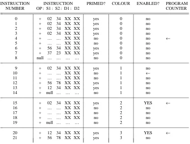
Fig. 10 Example code on one stream to show the operation of the sequencer.
Note. The opcodes in this example are “add” except for the null operations. The values in the source 1 and source 2 fields are only used to show their presence, their value is meaningless in this example. Also, the value of the destination addresses is not shown.
The instructions on the prototype MUSE resemble the five-field activity tem-plates described in Section 3.1. The destination addresses (D1 and D2) and the two source fields (S1 and S2) are a physical implementation of the “up arrow” and “down arrow” abstract signalling mechanism.
A colour program counter may have an initial value anywhere in the address range of the stream. The initial values of the program counters are loaded when the program is loaded. A colour is separated from another colour by at least one NULL instruction. No operands will be supplied for null instructions and so once a program counter reaches a null instruction that colour will be effectively stopped — the colour is said to be HALTED. (When all colours on all streams have halted the execution of the program should be complete).
Referring to Fig. 10, the code for colour 0 has been executed up to instruction 3 but is now awaiting operands for instruction 4 and so colour 0 is halted. Colour 1 is in a similar position, its first instruction 9 has been executed but it is halted on instruction 10.
and so instruction 15 will be selected and sent to the processor for execution. The program counter for colour 2 is then incremented by one.
The cycle will now start again. The sequencer checks all the instructions pointed to by the colour program counters starting with colour 0. Although colour 0 was halted on the last cycle it is possible that new operands have arrived for instruction 4 in which case colour 0 will be able to go. If operands have not arrived for instruction 4 then the sequencer will try colour 1 and then 2 and so on as before.
If there are no enabled instructions on any of the colours then the sequencer will go into a standby mode waiting for new operands to arrive from the match-ing store. The MUSE sequencer therefore has the ultimate control over the instruction sequence operation, but which particular environment is executed at any instant is determined by the arrival of priming operands from the Matching Store.
If a program fails then the current state of operation of the program may be determined by reading the program counters.
5.3.
InterruptsThe above architecture lends itself very readily to handling interrupts. This is achieved by allocating the highest priority colours (0, 1, 2 etc.) to interrupt rou-tines. The sequencer will ensure that they are executed as soon as interrupts occur.
§6.
Present StatusIn order to achieve a working prototype in a short time, some of the abstract ideas inherent in Fig. 6 have had to be implemented in a very concrete fashion. Commands such as↑0 occurring on stream 2 have to be translated by an assem-bler and loader into an explicit memory reference for insertion into one of the destination fields of the appropriate instruction. The absence of any kind of indexing registers or of the ability to transmit results to logical stream and environment numbers is a restriction of the present implementation, which it is hoped to remove in future developments. It implies that absolute addresses have to be computed at load time, which in turn puts a heavy burden on compilers and assemblers. Nevertheless a compiler has been written which accepts simple arithmetic expressions and which generates output code for the MUSE. An assembler is also available for low level testing.
A prototype (Mark 0) version of the MUSE machine has been built possess-ing 4 streams and 16 environments. It ran its first programs in July 1984. The prototype machine has a pipelined ring architecture of similar design to other data flow machines. The processor for each stream is constructed from AMD bit slice components whilst the sequencer is constructed from SSI and MSI logic cir-cuits.
operation of the prototype hardware. When this is completed it will be used to try out variations for future development of the architecture. At present data is being accumulated from the performance of the Mk. 0 which will be used in simulation studies prior to designing a Mk. 1 version of MUSE.
§7.
ConclusionThe prototype MUSE Mk. 0 with its associated compiler and assembler software has performed gratifyingly well and it has been found that the horizon-tal structure afforded by the streams, together with the vertical subdivisions of each stream into environments provides a target machine which accords well with the natural hierarchies found within programming constructs. The flexible address boundaries of the environments on each stream allow a program or expression to be mapped onto the machine without difficulty and a high degree of parallel execution to be achieved.
The problems encountered were, for the most part, foreseeable as conse-quences of the compromises needed to bring a prototype into operation quickly. The external bus structure between the streams is of a time multiplexed nature and whilst this is sufficient for the traffic in the Mk. 0 machine it is clear that such a simple scheme would not scale up much further. The whole aspect of communication between streams is being investigated, in particular the use of intra-stream communication to reduce communication requirements. Work con-tinues on these problems and into the further development of software for archi-tectures of this kind.
Acknowledgements
We thank the other members of the MUSE project team (Leon Harrison, David Allsopp and Neil Barrett) for many lively discussions conducted fre-quently, but not invariably, within the confines of Licensed Premises.
The construction of the hardware was financed by Plessey Office Systems, Beeston, Nottingham to whom we are also grateful, in conjunction with the Sci-ence and Engineering Research Council of Great Britain, for the provision of a CASE studentship for James Duckworth.
References
1) Backus, J., “Can programming Be Liberated from the von Neumann style? A Func-tional Style and Its Algebra of Programs,” Communications of the ACM, 21, 8, pp. 613–640. August, 1978.
2) Backus, J. W., Beeber, R. J., Best, S., Goldberg, R,, Haibt, L. M., Herrick, H. L., Nelson R. A., Sayre, D., Sheridan, P. B., Stern, H.. Ziller, I., Hughes, R. A.. and Nutt. R., “The FORTRAN automatic coding system.” in Proc. Western Joint Computer
Conf., Los Angeles, 1957.
and Hohensee, P., “SISAL : Streams and Iterations in a single-assignment language,”
Language reference manual version 1-1, Report M-146, Lawrence Livermore
Na-tional Laboratory.
4) INMOS. occamtmProgramming Manual, Prentice-Hall, 1984.
5) Watson, I. and Gurd, J. R., “A practical Dataflow Computer,” IEEE Computer, 15,
2, pp. 51–57, February, 1982.
6) Browning, S, A., “The Tree Machine,” Ph. D. Thesis, Computer Science Dept. Cali-fornia Institute of Technology, 1980.
7) Darlington. J, and Reeve, M.J., “Alice: A Multiprocessor Reduction Machine for Applicative Languages,” Proc. ACM/IMIT Conference on Functional Languages
and Computer Architecture, 1981.
8) Treleaven, P. C., Brownbridge, D. R., and Hopkins, R. P., “Data-Driven and Demand-Driven Computer Architecture,” Computing Surveys, 14, 1, pp. 93–143, March, 1982. 9) “Data Flow Systems,” Computer, 15, 2, February, 1982.
10) Karp, R. M. and Miller, R. E., “Properties of a model for parallel computations: Determinacy, Termination, Queueing,” SIAM J. Applied Mathematics, 14, 6, pp. 1390–1411, November, 1966.
11) Dennis, J. B., Boughton, G. A., and Leung, C. K. C., “Building Blocks for Data Flow Prototypes,” Proceedings of 1980 Symposium on Computer Architecture, pp. 1–8, 1980.
12) Arvind, Kathail, V., and Pingali, K., “A Dataflow Architecture with Tagged tokens,”
Internal report, MIT/LCS/TM-174, Laboratory for Computer Science, MIT.
September, 1980.
13) Suzuki, T., Tanaka, H., and Moto-oka, S., “Control Systems for ‘Topstar’ data flow machines and an evaluation thereof,” Proceedings Annual Conference Japan
In-formation Processing Society, pp. 85–86, May, 1980.
14) Dennis, J. B., “Data Flow Supercomputers,” Computer, pp. 48–56, November, 1980. 15) Weng, K. S., “Stream-Oriented Computation in Recursive Data-Flow Schemas,” M. S.
Thesis, Massachusetts Institute of Technology, October, 1975.
16) “The Texas Instruments TMS 9900, TMS 9980. and TMS 9940 Products,”" in Osborne
16-bit Microprocessor handbook (A. Osborne, and G. Kane, eds.), pp. 3.1–3. D17,