Magnetohydrostatic modelling of stellar coronae
D. MacTaggart,
1‹S. G. Gregory,
2T. Neukirch
3and J.-F. Donati
4 1School of Mathematics and Statistics, University of Glasgow, Glasgow G12 8QW, UK2SUPA, School of Physics and Astronomy, University of St Andrews, St Andrews KY16 9SS, UK 3School of Mathematics and Statistics, University of St Andrews, St Andrews KY16 9SS, UK 4LATT-UMR 5572, CNRS & Univ. Paul Sabatier, 14 Av. E. Berlin, F-31400 Toulouse, France
Accepted 2015 November 17. Received 2015 November 11; in original form 2015 September 30
A B S T R A C T
We introduce to the stellar physics community a method of modelling stellar coronae that can be considered to be an extension of the potential field. In this approach, the magnetic field is coupled to the background atmosphere. The model is magnetohydrostatic and is a balance between the Lorentz force, the pressure gradient and gravity. Analytical solutions are possible and we consider a particular class of equilibria in this paper. The model contains two free parameters and the effects of these on both the geometry and topology of the coronal magnetic field are investigated. A demonstration of the approach is given using a magnetogram derived
from Zeeman–Doppler imaging of the 0.75 MM-dwarf star GJ 182.
Key words: MHD – methods: analytical – stars: coronae – stars: magnetic field.
1 I N T R O D U C T I O N
The atmospheres of cool stars are governed by their magnetic fields. Phenomena ranging from flares to coronal mass ejections (CMEs) to stellar winds are all intimately related to the atmospheric mag-netic field. The best case study we have for a stellar magmag-netic field is the Sun. The solar magnetic field has been studied in detail over many scales and cycles. We cannot, however, observe the atmo-spheric (coronal) magnetic field directly and so must rely upon theoretical models. As input to these models, information about the magnetic field at the Sun’s surface (photosphere) can be determined through the Zeeman effect (Priest1982). Maps of the line-of-sight magnetic field (magnetograms) have been available for many years. More recently, vector magnetograms of the Sun have also been in-corporated into coronal models (e.g. Wiegelmann & Sakurai2012; R´egnier2013).
On stars other than the Sun, we now have insight into magnetic field structures. We can use Zeeman–Doppler Imaging (ZDI) to de-termine stellar magnetograms (e.g. Donati et al.2008). Such mag-netograms convey only the large-scale structure of a star’s magnetic field. Fields on the active region scale and smaller are not observable currently. Much important information about the stellar environ-ment, however, can be gained from a knowledge of the large-scale structure of the global magnetic field. Two approaches have been used mainly to study the magnetic coronae of stars (henceforth, ‘stars’ refers to stars other than the Sun). The first is a potential field extrapolation (e.g. Jardine, Collier Cameron & Donati2002; Gregory & Donati2011; Lang et al.2012). The potential field
E-mail:[email protected]
proach is useful as it gives a unique solution that minimizes the magnetic energy for a given set of boundary conditions. However, as there is no current (j=0) in a potential field, the magnetic field in the corona does not contain twist, which is considered important for the onset of different forms of eruptive behaviour (e.g. Hood, Ar-chontis & MacTaggart2011). Also, the Lorentz force completely decouples from the non-magnetic terms in the magnetohydrody-namic (MHD) momentum equation. This decoupling means that certain assumptions need to be made when finding proxies for quan-tities such as X-ray emission (e.g. Jardine, Gregory & Donati2008). The second approach is to perform a full MHD simulation of the global corona (e.g. Riley et al.2006; Cohen et al.2010; Romanova et al. 2010; Vidotto et al. 2011), where it is possible to capture the large-scale dynamics of the corona. However, this approach is computationally very expensive and often requires supercomputing resources.
In this paper, we introduce a technique that can be thought of as an intermediary step between the potential field model and full MHD simulations, as mentioned above. We present a magnetohydrostatic (MHS) solution which couples the coronal density, pressure and magnetic field together. Perturbations in the hydrostatic density and pressure, due to the magnetic field, can be calculated self-consistently. As the solution is static, like the potential field model, it is very simple to implement. The model allows us to calculate, with relative ease, a twisted stellar coronal field where magnetic forces balance hydrostatic forces. The approach presented in this paper has been applied to the solar corona where large-scale features have been captured successfully (Bogdan & Low1986; Neukirch1995; Zhao, Hoeksema & Scherrer2000; Ruan et al.2008). Our approach will be particularly suited to stellar applications, where magnetograms only convey the large-scale structure of the magnetic field. This type
at University of St Andrews on January 25, 2016
http://mnras.oxfordjournals.org/
of model can capture the large-scale field structure (as evidenced by the solar applications mentioned above) and improve upon the potential field extrapolations with the inclusion of current density and the coupling of the magnetic field to the background stellar atmosphere.
In the following section, we give a detailed derivation of the coronal magnetic field and the associated density and pressure per-turbations (correcting typographical errors that appear in previous works). We follow this section with an analysis of how the resulting free parameters affect the geometry and topology of the model coro-nal magnetic field. After the acoro-nalysis, an application of the model is given where a magnetic map of the M-dwarf GJ 182, published by Donati et al. (2008), is used as input. The paper ends with a summary.
2 AT M O S P H E R E M O D E L
2.1 Magnetic field
The MHS equations that describe the balance between the Lorentz and hydrostatic forces can be written as
j×B− ∇p−ρg=0, (1)
∇ ×B=μ0j, (2)
∇·B=0. (3)
Here,Bis the magnetic induction (referred to as the magnetic field),
j is the current density,pis the plasma pressure,ρis the plasma density andgis gravity. A discussion of appropriate boundary con-ditions will be left until later. Rather than proceeding with equations (1) to (3) in dimensional form, we write them in dimensionless form by introducing the variables
r =r0r∗, B=B0B∗, g=g0g∗,
p =(B0/μ0)p∗, ρ=B02/(μ0r0g0)ρ∗,
j =B0/(μ0r0)j∗. (4)
The distance vector is labelledrin anticipation of the use of spher-ical coordinates for stellar applications. Dropping the asterisks, the dimensionless MHS equations are
j×B− ∇p−ρ∇ψ =0, (5)
∇ ×B= j, (6)
∇·B=0. (7)
All further expressions will be in dimensionless form unless stated otherwise. Here, we have written gravity in terms of its potentialψ, viz.
ψ = −1r, (8)
To make progress, we model the current density as the composition of two distinct terms:
j=αB+ ∇ ×(Fr). (9)
This choice of the current density enables us to model the magnetic field through a range of plasmaβ(=2μ0p/B2
0). Since equation (9)
is linear, we can make analytical progress and take a practical inter-mediate step between potential field extrapolations and expensive
global MHD simulations.αis a constant parameter and the first term on the RHS of equation (9) represents the current density of a linear force-free field. The second term on the RHS represents the current density that produces a Lorentz force that can balance the effects of the pressure gradient and gravity.Fis a free function which will be specified shortly. The approach of using this type of term was introduced by Low (1982) and has been used in several subsequent studies (e.g. Low1991; Gibson, Bagenal & Low1996; Neukirch & Rast¨atter1999; Petrie & Neukirch2000). Jardine et al. (2013) also present a non-potential magnetic field model, in the stellar physics context, with a term similar to the second term on the RHS of equation (9). However, they do not consider MHS equilibria. The combination of the two terms in equation (9) results in components of current density that are both parallel and perpendicular to the magnetic field. Therefore, the total field-aligned current density, if written in the form ¯αB, has a non-uniform ¯α. Although the field in our model can be (depending on the choice of parameters discussed below) more complicated than a linear force-free field, our model has the advantage of taking the same input from magnetograms as linear force-free models. As potential field models are a particular case of linear force-free models (α=0), potential models can be updated to the MHS model easily.
The following derivation of the model is based on Bogdan & Low (1986) and Neukirch (1995). An alternative method exploiting the toroidal and poloidal components of the field can also be used (Neukirch & Rast¨atter1999). We shall utilize the toroidal–poloidal approach later when studying the topology of the field.
Inserting equation (9) into Amp`ere’s law, equation (2), gives, after some manipulation,
r·(∇ × ∇ ×B)=α2r·B+r·∇ ×(∇F×r), (10)
whereris the radial vector. Further, we choose the form ofFto be
F=ξ(r)r·B, (11)
whereξ(r) is a free function. The particular form ofξ(r) will be chosen later to allow for an analytical solution. At this point it is useful to introduce the angular momentum operator
L≡ −ir× ∇. (12)
This operator is common in quantum mechanics and a description of its properties can be found in Jackson (1975). By simple manip-ulation, it can be shown that
r·(∇ × ∇ ×B)= −∇2(r·B). (13)
Combining equations (10) and (13), and making use of equations (11) and (12), gives
∇2
(r·B)+ξ(r)L2(r·B)+α2(r·B)=0. (14)
To proceed, we expandr·Bin spherical harmonics,
r·B=
∞
l=1
l
m=−l
l(l+1)QlmYlm(θ, φ), (15)
where
Qlm=
2
j=1 A(j)
lmu(lj)(r). (16)
A(j)
lm are constant (complex) coefficients. To determine theu(lj)(r),
inserting equation (15) into equation (14) gives
d2
dr2−l(l+1)
1
r2−ξ(r)
+α2
g(j)
l =0, (17)
at University of St Andrews on January 25, 2016
http://mnras.oxfordjournals.org/
wheregl(j)=ru(lj). In deriving equation (17), use has been made of the property
L2Ym
l (θ, φ)=l(l+1)Ylm(θ, φ). (18)
To solve equation (17) analytically, a particular form must be chosen forξ(r). Notice that equation (17) has the form of a 1D Schr¨odinger equation withξ(r) playing the role of the potential (e.g. Rae2002). This analogy gives us a starting point for what formξ(r) can take in order to yield analytical solutions. Several possible analytical solutions are discussed in Neukirch (1995). Following Ruan et al. (2008), we adopt
ξ(r)= 1
r2−
1
(r+a)2, (19)
whereais a free parameter. This particular form represents the contribution of the non-force-free part of the current density decay-ing with height, as in the low solar corona (e.g. Gary2001). By considering the following variable transformation
s=r+a, f(j)
l =
g(j)
l
s1/2, (20)
equation (17) transforms into Bessel’s equation
d2
ds2+
1
s
d ds +α
2−(l+1/2) 2
s2
f(j)
l =0. (21)
Converting back to the original variables, the solutions can be writ-ten as
u(1)
l =
√
r+a
r Jl+1/2(α(r+a)), (22)
u(2)
l =
√
r+a
r Nl+1/2(α(r+a)), (23)
whereJl+1/2andNl+1/2are Bessel functions of the first and second
kind, respectively.
Before writing down an expression for the magnetic field, we re-quire theA(lmj)which are determined using the boundary conditions and an orthogonality constraint. As mentioned earlier, the solutions of the MHS equations (1)–(3) require boundary conditions. In this problem, the required boundary conditions are the radial compo-nents of the field at the stellar surface and a source surface. At the stellar surface, the radial magnetic field component is provided by a magnetogram. The modeller is free to select an appropriate form for the source surface and choose the distance of the source sur-face from the stellar sursur-face. In solar applications,in situsatellite observations can constrain the form of the source surface. No such constraints exist for stellar coronae, although X-ray observations can be used to provide loose constraints (e.g. Hussain et al.2007). For MHS models, the effects of outflows (e.g. stellar winds) are in-corporated into the form of the source surface. At the stellar surface
r=1 (we have takenr0=R∗) the radial component of the field,
B1
r, can be written as
B1
r(θ, φ)=
∞
l=1
l
m=−l
l(l+1)Q1lmYlm(θ, φ), (24)
where
Q1
lm=A(1)lm
√
1+aJl+1/2(α(1+a))
+A(2)
lm
√
1+aNl+1/2(α(1+a)). (25)
Note that if the magnetogram comes from observations, it is im-portant to ensure that the magnetic flux is balanced. Using the orthogonality condition
π
θ=0
2π
φ=0 Ym
l Y¯lm sinθdθdφ=δllδmm, (26)
we find
Q1
lm=
1
l(l+1)
π
θ=0
2π
φ=0 B1
r(θ, φ) ¯Ylmsinθdθdφ. (27)
Here, the overbar represents the complex conjugate. Equation (27) is a linear equation forA(1)lmandA(2)lm. Applying the same procedure at the source surface, or imposing another constraint, results in another linear equation and this system can be solved to find the coefficientsA(lmj).
To find a closed-form solution for the magnetic field, we take the dot product ofrand equation (6) and apply the angular momentum operator,
L·B= −iαr·B. (28)
From the definition ofL in equation (12), equation (28) contains only derivatives ofBθandBφ. Hence, we can write
L·BT = −iα
∞
l=1
l
m=−l
2
j=1
l(l+1)A(lmj)ul(r)(r)Ylm(θ, φ), (29)
where BT =Bθeθ+Bφeφ. We require a series expansion of BT
to match the RHS of equation (29). Following Jackson (1975) and Neukirch (1995), we find
BT =
∞
l=1
l
m=−l
vlm(r)LYlm(θ, φ)+wlm∇Ylm(θ, φ). (30)
The unknown functions vlm(r) andwlm(r) can be found by two
simple considerations. For brevity, we shall consider a single order forlandm. Inserting equation (30) into equation (29) and making use of equation (18) results in
vlm(r)= −iα
2
j=1 A(j)
lmu(lj)(r). (31)
On the application of equation (7), and some simple rearrangement, we find
wlm=
2
j=1 A(j)
lm
d dr
ru(j)
l (r) . (32)
The expression for the global coronal magnetic field is then given by
B=
∞
l=1
l
m=−l
2
j=1 A(j)
lm
l(l+1)u(lj) r
r2Y
m l (θ, φ)
− iαu(j)
l LYlm(θ, φ)+
d dr
ru(j)
l ∇Ylm(θ, φ)
. (33)
The spherical components of equation (33) are listed in Appendix A.
2.2 Non-magnetic variables
We now consider what forms the pressure and density take in the MHS model. Inserting the model current density, given by equation
at University of St Andrews on January 25, 2016
http://mnras.oxfordjournals.org/
(9), into the force balance equation (5) gives, after some rearrange-ment,
∇p+ρ∇ψ+(B·r)∇F−(B·∇F)r=0. (34)
For a non-trivial current density, we require ∇F and r to be linearly independent. Hence, equation (34) implies that p=
p(r, F). Considering the component in the direction∇F, we obtain
∂p ∂F
r
= −B·r= − 1
ξ(r)F . (35)
Integrating equation (35) yields
p=p0(r)−
1
2ξ(r)(r·B)
2.
(36)
p0is the background pressure and is found from hydrostatic
bal-ance. The second term in equation (36) is due to the non-force-free component in the current density.
By considering ther-component of equation (34), the density is found to be
ρ=ρ0(r)+r2
1 2
dξ dr(r·B)
2+rξB·∇(r·B)
. (37)
Here,ρ0(r) is the background hydrostatic density profile.
3 A N A LY S I S
In this section, we analyse the effects of the free parameters,αanda, on the geometry and topology of the coronal magnetic field. These parameters determine the form of the two model current density terms given in equation (9).
3.1 Free parameters and field geometry
The main assumption of the MHS model is the form of the current density in equation (9). The first term that contributes to the current density,αB, represents the linear force-free part of the current that is parallel to the magnetic field. This term is well known for adding twist to the magnetic field. Analogous to vorticity in a sheared flow, current density can manifest itself through a sheared magnetic field. To demonstrate this effect, we shall consider a dipolar field with very simple boundary conditions. These are
Br(R, θ, φ)=cosθ, B(RSS, θ, φ)=0, (38)
whereR=1 is the stellar surface andRSS=3 is the source surface.
Fig.1shows the coronal magnetic field with boundary conditions (38) and free parametersα=0.5 anda=0.1. The effect ofα= 0 can be seen clearly. Moving from the stellar surface upwards, the alignment angle of the magnetic arcades changes. This shearing of the magnetic field is evidence of non-zero current.
The second term in equation (9) is perpendicular to gravity (the radial direction). It is this term that couples the magnetic field to the plasma pressure and density. The second term depends on both of the free parametersαanda. As mentioned above, increasing the magnitude of αincreases the twist (positive and negative values determine the sense of the twist). The effect of changingarequires more investigation. Zhao et al. (2000) perform several numerical experiments and show that increasing the value ofacauses magnetic arcades to expand. Physically, this expansion occurs if there is an increase in magnetic pressure. Consider equation (36) re-written as
p+pm=p+ 1
2ξ(r)(r·B)
2=p
[image:4.595.309.548.55.201.2]0, (39)
Figure 1. Field line plot of the dipolar field specified in equation (38). The free parameters areα=0.5 anda=0.1. Low magnetic arcades are aligned at different angles to those that rise to greater radial distances. This shearing of the field is due to a non-zeroα. The coloured stellar surface shows the non-dimensionalBrcomponent of the dipolar field in equation (38).
Figure 2. The variation of the signed maximum magnitude of the pressure perturbationpmas a function ofafor fixedα=0.3. Values on the axes are
non-dimensional as specified in equation (4).
wherepis the plasma pressure,pmis the magnetic pressure
pertur-bation andp0is the background hydrostatic pressure of the stellar
atmosphere. By considering the expression for the pressure pertur-bation, the sign ofpmdepends on the sign ofξ(r). From equation
(19), the sign depends, in turn, on the choice ofa.pmalso depends
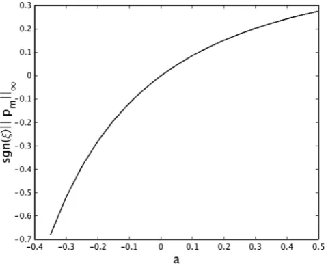
onathrough equations (22) and (23). To give an illustration of how the pressure perturbation depends on a, we calculate the signed maximum perturbation, sgn(ξ)pm∞. This quantity can be found
analytically as
sgn(ξ)pm∞= 1
2ξ(1)= 1 2
1− 1 (1+a)2
, (40)
using the fact that the maximum magnitude of the pressure pertur-bation occurs at the stellar surface wherer·B∞=1. Fig.2shows a plot of equation (40).
For a>0, the values are positive, indicating an expansion of the magnetic field (e.g. Zhao et al.2000). Whena<0,pmis also
negative, resulting in compression of the magnetic field. What this analysis shows is that the choice ofξ(r) is crucial for determining
at University of St Andrews on January 25, 2016
http://mnras.oxfordjournals.org/
[image:4.595.307.546.274.467.2]how the pressure perturbation will behave. The pressure perturba-tion, in turn, will influence the inflation of the magnetic field.
3.2 Magnetic helicity
Magnetic helicity is a topological invariant of ideal MHD (e.g. Biskamp1997) and can be interpreted as the average pairwise link-age of magnetic field lines (Arnold & Khesin1992). The magnetic helicity is defined by
H =
V
B·AdV , (41)
whereA= ∇ ×BandVis the volume of concern. This quantity is only gauge-invariant, however, if the magnetic field is closed, that is ifB·n=0 on∂V. For the magnetic fields described in this paper, this condition is not met as field leaves the stellar surface and either returns back down to this level (closed field) or connects to the source surface above (open, stellar wind bearing, field). Berger & Field (1984) show that a gauge-invariant measure of helicity is also possible for open magnetic fields. This form of helicity is known as relative helicity and can be written as
HR=H(BV,BV−,BV+)−H(BrefV ,BV−,BV+), (42)
where
H(BV1, . . . ,BVn)= n
i=1
Vi
BVi·AVidV . (43)
Here,Vis the volume between the stellar surface and the source surface and V− and V+ represent volumes below and above V, respectively. The magnetic fields in these two volumes match the field ofVat its boundaries and close to allow for helicity to be a topological invariant. Berger & Field (1984) show that the magnetic fields inV−andV+can be ignored and that helicity only requires knowledge of the field inV. The required magnetic fields areBV, the coronal magnetic field found from equation (33), andBref
V, a
reference magnetic field with the same boundary conditions asBV. The reference field is normally taken to be a potential magnetic field for simplicity. Relative helicity can then be thought of as a quantitative measure of how ‘different topologically’BV is from
Bref
V .
IfBV−andBV+are chosen to be potential, the relative magnetic
helicity reduces to
HR=H(BV,BV−,BV+), (44)
in a spherical geometry. In order to determine an expression forHR,
we proceed by decomposing the magnetic field into poloidal (P) and toroidal (T) components
B= ∇ × ∇ ×(Pr)+ ∇ ×(Tr). (45)
The magnetic field in equation (45) can be written as
B= −i[∇ ×(LP)+LT]. (46)
The vector potential is found to be
A= −i[LP+rT+ ∇λ], (47)
whereλis an arbitrary gauge function. The relative helicity can be expressed in the appealing form
HR= −2
VLP·LTdV , (48)
[image:5.595.309.549.57.242.2]which reflects the fact that helicity arises due to the linkage of the poloidal and toroidal magnetic field. Equation (48) (in a slightly
Figure 3. The variation of relative helicityHRas a function ofafor different
values ofα. Key: solid,α=0.5; dashed,α=0.1; dotted,α=0; dot–dashed, α= −0.2. Values on the axes are non-dimensional as specified in equation (4).
different form) is derived in Berger (1985) and so we do not repeat the derivation here. Berger (1985) then goes on to find an expression for the relative helicity of linear force-free fields. We shall now proceed in a similar manner and find an expression for this class of MHS equilibria. Inserting equation (45) into equation (9), we can derive the equations
∇2P+αT +F=
0, T−αP=0, (49)
which can be reduced to
∇2P+α2P +F=0. (50)
Using equation (45), we can show that
L2P =r·B. (51)
ApplyingL2to equation (50) and using the distributive property of L2, we obtain
∇2(r·B)+ξ(r)L2(r·B)+α2(r·B)=0, (52)
which is just equation (14). Hence, one can expandPas
P = ∞
l=1
l
m=−l
QlmYlm(θ, φ). (53)
Following Berger (1985), after integration by parts, equation (48) with suitable substitutions becomes
HR=2α
∞
l=1
l
m=−l l(l+1)
RSS
R∗
|Qlm|2r2dr, (54)
whereR∗is the stellar radius andRSSis the radius of the source
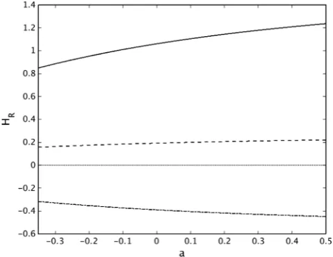
surface. To investigate the dependence of the relative helicity on the free parameters, we determine equation (54) for the dipolar field with boundary conditions specified in equation (38). Fig.3displays howHRvaries as a function ofafor different values ofα.
The curves in Fig.3can be interpreted as how much the field is ‘different topologically’ from a potential field with the same boundary conditions. Forα=0,Hr=0, as shown by the dotted
line in Fig.3. If there is no twist injected into the field, throughα, then the field is topologically equivalent to a potential field and so
HR=0. Forα >0, the relative helicity increases monotonically
at University of St Andrews on January 25, 2016
http://mnras.oxfordjournals.org/
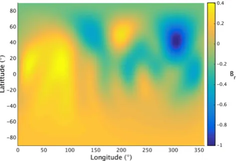
Figure 4. Magnetogram of GJ 182.Brhas been normalized with respect to
its largest magnitude (355 G).
witha. Forα <0,|HR|also increases monotonically but now the
sign of the relative helicity is negative. In the range of the parameter space displayed in Fig. 3, the effect of increasing bothaand α is to increase the magnitude of the relative helicity. This result occurs because increasing the free parametersaandα increases the current density which, in turn, moves the field further from a potential state. For much higher values ofα, resonances can occur where the magnetic helicity and magnetic energy go to infinity (Berger1985). These large values, however, are not applicable to our model which is concerned with large-scale stellar fields that are not twisted to such extents (e.g. Zhao et al.2000).
4 A P P L I C AT I O N
To illustrate the model, we apply it to the young single M-dwarf GJ 182 (M∗=0.75 M,R∗=0.82 R,Prot=4.35 d; Donati et al.
(2008)). This star shows evidence for surface differential rotation, with the equatorial regions rotating faster than the poles. The mag-netic field is dominantly toroidal with a mostly non-axisymmetric poloidal component (Donati et al.2008), consistent with a partially convective interior (Gregory et al.2012). As input to the model, we take GJ 182’s magnetogram, the radial component of the magnetic field at the stellar surface. The magnetogram is shown in Fig.4
where the field is normalized with respect to its largest magni-tude, 355 G. This star has been chosen to demonstrate the model because the star’s magnetic field differs from the large-scale sym-metric dipolar structure of the solar magnetic field. Also, GJ 182’s coronal magnetic field has been modelled by Lang et al. (2012) using a potential field extrapolation. This previous study allows us to make a comparison and highlight the extra features that appear in our model.
To complete the model, an outer boundary condition, the source surface, is required. As mentioned previously, the radial position and form of the source surface are modelling choices. For simplicity, we take the dipolar radial field
Br(r=4)=βY10(θ, φ), (55)
whereβ=O(r−3). With these radial boundary conditions, the
mag-netic field in the region 1<r<4 can be calculated using equation (33). We takel=8, which is enough to capture the features of the magnetogram. In the last section, we discussed some of the effects of the free parameters. For applying the model to GJ 182, we choose
[image:6.595.45.282.57.218.2]α=0.4 anda=0.3. This choice lies in the part of the parameter
Figure 5. A field line extrapolation usingα=0.4 anda=0.3. The contour map showsBr. Sigmoidal field lines are representative ofj=0. Field lines
are multicoloured to make them easier to visualize.
space where the magnetic pressure is increased, resulting in a pres-sure deficit due to the magnetic field. A visualization of the coronal field is shown in Fig.5where several field lines are plotted and the sphere shows the map ofBrgiven in Fig.4. As mentioned above,
Lang et al. (2012) plot a potential field extrapolation of the corona of GJ 182. The orientation of the star in Fig.5is chosen to be similar to that shown in Lang et al. (2012) for ease of comparison.
Although the source surface will help to determine the behaviour of open field lines, its influence on the geometry of lower closed field lines is smaller as such is determined primarily by the form of the current density. Looking at the field lines between the large positive and negative regions ofBr, the arcades are sheared. That
is, the low field lines at the polarity inversion line are at a different angle to those above. As mentioned before, this effect is due to a non-zero current. The twist of the field due to the linear force-free term can also be seen in the sigmoidal shape of the field lines. This shape is most clearly visualized in Fig.5by the higher field lines of the sheared arcade. Reducing the magnitude ofαwould result in field lines becoming straighter, i.e. losing their sigmoidal shape. In the potential extrapolation of Lang et al. (2012), the arcade field lines do not possess a sigmoidal shape asα=0 in their case. The expansion of the field lines can be controlled bya, as described previously.
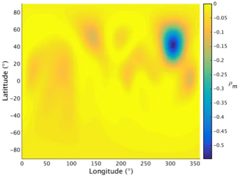
To see the effects of the coronal magnetic field on the back-ground atmosphere, we have constructed maps of the density and pressure perturbations at the stellar surface. Fig.6shows the density perturbation, the second term on the RHS of equation (37).
In the magnetogram for GJ 182 (Fig.4), the radial field in the Northern hemisphere contains concentrations that alternate in sign. Beginning with a positive concentration, this changes to negative with increasing longitude. Moving further around the star in lon-gitude, the positive to negative pattern repeats. This pattern is also revealed in the density perturbation map. From equation (37) the density perturbation is proportional toB2
r. Hence, the stronger the
magnetic polarity, the greater the density perturbation. The pressure perturbation map, shown in Fig.7, is very similar to the density per-turbation map. Again, this quantity, the second term on the RHS of equation (36), is proportional toB2
r. The only significant difference
between the two maps is the magnitude of the perturbations.
at University of St Andrews on January 25, 2016
http://mnras.oxfordjournals.org/
Figure 6. The density perturbation, ρm=r2[ξ(r)(r·B)2/2+ rξ(r)B·∇(r·B)], at the stellar surface. Values on the colour scale are non-dimensional as specified in equation (4).
Figure 7. The pressure perturbation,−pm= −ξ(r)(r·B)2/2, at the stellar surface. The values are negative as we are considering the perturbation to the hydrostatic pressure, shown in equation (36). Values on the colour scale are non-dimensional as specified in equation (4).
5 S U M M A RY
In this paper, we have presented, analysed and demonstrated a MHS model for stellar coronae. The model extends the popular potential field model to allow for the magnetic field to contain current and couple to the background density and pressure. The main assump-tion of the model is the choice for the current density, which is split into a linear force-free part and another part that links the field to the background atmosphere. The model, given by equation (9), has its particular form so that Amp`ere’s law (2) is linear and analytical progress is possible. The MHS equations then boil down to solv-ing Bessel’s equation subject to a model choice forξ(r). In this paper, we have chosen a form that allows for analytical progress. Other choices that allow for analytical solutions are also possible (e.g. Neukirch1995). Of course, more complicated expressions for
ξ(r) can be specified but will require a numerical treatment (e.g. MacTaggart et al.2013). A closed-form expression for the coro-nal magnetic field is found and the associated perturbations to the background hydrostatic pressure and density are also determined.
We present an analysis of the effects of the two free model param-eters. In terms of the geometry of the field, the parameterαincreases the shear/twist in the magnetic field. Increasing the magnitude of
αcreates field lines with a sigmoidal shape. The parameter ais related to the inflation of magnetic field lines through the magnetic pressure. The size of magnetic arcades can change depending on the choice ofa. The topology of the coronal field is studied by consid-ering the relative magnetic helicity. This quantity gives a measure of how different, topologically, the coronal field is compared to a potential field with the same boundary conditions (the choice of reference field in this paper). An expression for the relative helic-ity, for the class of MHS equilibria presented here, is determined. Increasing the magnitude ofαalso increases the relative helicity. This increase occurs because the current, and hence twist, increases in the magnetic field. Increasing the magnitude ofaincreases the relative helicity.
Finally, a simple demonstration of the model is given for the M0.5 dwarf star GJ 182. Field lines are plotted showing the non-potential features of the model. The density and pressure perturbations at the stellar surface are also displayed and are proportional toB2
rso that
shapes on the countour plots can be matched to corresponding ones on the magnetogram.
The model presented in this paper is suitable for determining the large-scale features of a star’s corona. The model also has the advantage of being simple, fast to implement and, unlike full MHD models, is not computationally expensive to implement. The effort involved is only slightly more than a potential field model (which is a special case of the MHS model). By a suitable choice ofξ(r) and the free parametersαanda, one can investigate stellar coronae with different geometries, topologies, pressure and density distributions and current density profiles. In future work, we will apply our model to stellar observations and attempt to constrain the free parameters using the information provided by the observations, such as the toroidal component of the magnetic field.
AC K N OW L E D G E M E N T S
SGG acknowledges support from the Science & Technology Facilities Council (STFC) via an Ernest Rutherford Fellowship [ST/J003255/1]. TN would like to acknowledge support from the STFC Consolidated Grant ST/K000950/1. The authors would like to thank J. Morin for helpful advice on the paper.
R E F E R E N C E S
Arnold V. I., Khesin B. A., 1992, Annu. Rev. Fluid Mech., 24, 145 Berger M. A., 1985, ApJS, 59, 433
Berger M. A., Field G. B., 1984, J. Fluid Mech., 147, 133
Biskamp D., 1997, Nonlinear Magnetohydrodynamics. Cambridge Univ. Press, Cambridge
Bogdan T. J., Low B. C., 1986, ApJ, 306, 271
Cohen O., Drake J. J., Kashyap V. L., Hussain G. A. J., Gombosi T. I., 2010, ApJ, 721, 80
Donati J.-F. et al., 2008, MNRAS, 390, 545 Gary A., 2001, Sol. Phys., 203, 71
Gibson S. E., Bagenal F., Low B. C., 1996, J. Geophys. Res., 101, 4813 Gregory S. G., Donati J.-F., 2011, Astron. Nachr., 332, 1027
Gregory S. G., Donati J.-F., Morin J., Hussain G. A. J., Mayne N. J., Hil-lenbrand L. A., Jardine M., 2012, ApJ, 755, 97
Hood A. W., Archontis V., MacTaggart D., 2011, Sol. Phys., 278, 3 Hussain G. A. J. et al., 2007, MNRAS, 377, 1488
Jackson J. D., 1975, Classical Electrodynamics. John Wiley & Sons New York
at University of St Andrews on January 25, 2016
http://mnras.oxfordjournals.org/
Jardine M., Collier Cameron A., Donati J.-F., 2002, MNRAS, 333, 339 Jardine M., Gregory S. G., Donati J.-F., 2008, MNRAS, 386, 688 Jardine M., Vidotto A. A., van Ballegooijen A., Donati J.-F., Morin J., Fares
R., Gombosi T. I., 2013, MNRAS, 431, 528
Lang P., Jardine M., Donati J.-F., Morin J., Vidotto A., 2012, MNRAS, 424, 1077
Low B. C., 1982, ApJ, 263, 952 Low B. C., 1991, ApJ, 370, 427
MacTaggart D., Elsheikh A., McLaughlin J. A., Simitev R. D., 2013, A&A, 556, A40
Neukirch T., 1995, A&A, 301, 628
Neukirch T., Rast¨atter L., 1999, A&A, 348, 1000 Petrie G. J. D., Neukirch T., 2000, A&A, 356, 735
Priest E. R., 1982, Solar Magnetohydrodynamics. Kluwer Academic Pub-lishers, Dordrecht, Holland
Rae I. M., 2002, Quantum Mechanics. IOP Publishing Ltd, London, UK R´egnier S., 2013, Solar Phys., 288, 481
Riley P., Linker J. A., Miki´c Z., Lionello R., Ledvina S. A., Luhmann J. G., 2006, ApJ, 653, 1510
Romanova M. M., Long M., Lamb F. K., Kulkarni A. K., Donati J.-F., 2010, MNRAS, 411, 915
Ruan P., Wiegelmann T., Inhester B., Neukirch T., Solanki S. K., Feng L., 2008, A&A, 481, 827
Vidotto A. A., Jardine M., Opher M., Donati J.-F., Gombosi T. I., 2011, MNRAS, 412, 351
Wiegelmann T., Sakurai T., 2012, Living Rev. Solar Phys., 9, 5 Zhao X. P., Hoeksema J. T., Scherrer P. H., 2000, ApJ, 528, 932
A P P E N D I X A : S P H E R I C A L C O M P O N E N T S
The spherical components of the coronal magnetic field are
Br=
∞
l=1
l
m=−l
2
j=1 A(j)
lm l(l+1)
r u
(j)
l (r)Ylm(θ, φ), (A1)
Bθ =
∞
l=1
l
m=−l
2
j=1 A(j)
lm
α
sinθu
(j)
l (r)∂∂φYlm(θ, φ)
+ 1
r
d dr(ru
(j)
l (r))∂∂θYlm(θ, φ)
, (A2)
and
Bφ =
∞
l=1
l
m=−l
2
j=1 A(j)
lm
−αu(j)
l (r)∂∂θYlm(θ, φ)
+ r 1
sinθ d dr(ru
(j)
l (r))∂∂φYlm(θ, φ)
. (A3)
All terms are defined as in the main body of the paper.
This paper has been typeset from a TEX/LATEX file prepared by the author.
at University of St Andrews on January 25, 2016
http://mnras.oxfordjournals.org/