Surface flux patterns on planets in circumbinary systems and potential for photosynthesis

and Potential for Photosynthesis

Duncan H. Forgan

_{, Alexander Mead}

_{, Charles S. Cockell}

_{, John A. Raven}

August 25, 2014

1_{Scottish Universities Physics Alliance (SUPA), Institute for Astronomy, University of Edinburgh,}

Black-ford Hill, Edinburgh, EH9 3HJ, UK

2_{UK Centre for Astrobiology, School of Physics and Astronomy, University of Edinburgh}

3 _{Division of Plant Sciences, University of Dundee at TJHI, The James Hutton Institute, Invergowrie,}

Dundee, UK

First Draft

Word Count: 5700

Direct Correspondence to:

D.H. Forgan

Email:[email protected]

1

Abstract

Recently, the Kepler Space Telescope has detected several planets in orbit around a close binary star

system. These so-called circumbinary planets will experience non-trivial spatial and temporal

distribu-tions of radiative flux on their surfaces, with features not seen in their single-star orbiting counterparts.

Earthlike circumbinary planets inhabited by photosynthetic organisms will be forced to adapt to these

unusual flux patterns.

We map the flux received by putative Earthlike planets (as a function of surface latitude/longitude

and time) orbiting the binary star systems Kepler-16 and Kepler-47, two star systems which already

boast circumbinary exoplanet detections. The longitudinal and latitudinal distribution of flux is sensitive

to the centre of mass motion of the binary, and the relative orbital phases of the binary and planet. Total

eclipses of the secondary by the primary, as well as partial eclipses of the primary by the secondary add

an extra forcing term to the system. We also find that the patterns of darkness on the surface are equally

unique. Beyond the planet’s polar circles, the surface spends a significantly longer time in darkness than

latitudes around the equator, due to the stars’ motions delaying the first sunrise of spring (or hastening

the last sunset of autumn). In the case of Kepler-47, we also find a weak longitudinal dependence for

darkness, but this effect tends to average out if considered over many orbits.

In the light of these flux and darkness patterns, we consider and discuss the prospects and challenges

for photosynthetic organisms, using terrestrial analogues as a guide.

Keywords: Circumbinary, habitability, darkness, photosynthesis

1

Introduction

Extrasolar planets (or exoplanets) show a rich variety of orbital architectures, challenging planet formation

theory. Their properties force astrophysicists and astrobiologists to re-examine their assumptions regarding

the growth and evolution of potentially habitable planets in the Milky Way.

Typically, the astrophysical “habitability” of a world is determined by the radiative flux received from

an external radiation source. This flux is used as input for climate models, which simulate the response

of a planet of Earth mass - with similar composition and atmosphere - to this radiation. This allows the

construction of a habitable zone (HZ), a region surrounding the radiation source that should be capable of

hosting planets of Earth mass and composition with liquid water on their surface.

This habitable zone concept pre-dates the detection of exoplanets by several decades (Huang, 1959;

Hart, 1979), culminating in the seminal 1D radiative transfer calculations of Kasting, Whitmire & Reynolds

(1993), which defined inner and outer radial boundaries of a spherically symmetric HZ, based on the

star’s luminosity and effective temperature. These calculations would form the basis for a number of

parametrisations of the HZ (Underwood, Jones & Sleep, 2003; Selsis et al., 2007; Kaltenegger & Sasselov,

2011). Recently, Kopparapu et al. (2013) returned to Kasting et al’s original calculations, updating the

conservative case) to 0.99 and 1.7 AU respectively, although these boundaries apply only to Earth mass

planets - increasing the mass tends to move the inner boundary closer to the star (Kopparapu et al., 2014).

The HZ model has been strongly challenged since the first detection of an exoplanet in a main sequence

star system (Mayor & Queloz, 1995). For example, the orbital eccentricity of exoplanets is often much

higher than exhibited in the Solar System, allowing planets to move in and out of the HZ over the course

of an orbit. The habitability of a world then becomes a function of the length of time it spends inside the

zone (Williams & Pollard, 2002; Kane & Gelino, 2012; Kane et al., 2012).

The advent of the Kepler Space Telescope has allowed, for the first time, meaningful statistical

discus-sion of how frequently stars in the Milky Way possess planets in the HZ (Dressing & Charbonneau, 2013;

Petigura, Howard & Marcy, 2013; Kasting et al., 2013). These analyses are generally sensitive to

prop-erties such as stellar mass, and the precise definition of the inner and outer HZ boundaries, which are in

turn sensitive to properties such as the planet’s surface liquid water fraction and atmospheric composition.

Nevertheless, the above authors find the frequency of “Earth-like” planets around other stars to range from

about 15% to as high as 50%.

One of Kepler’s achievements which deserves note is the first detection of planetary systems orbiting

binary main sequence stars. These possess planets in orbit of the centre of mass of a binary system. They

are commonly referred to as P-type or circumbinary systems, in contrast to S-type systems where planets

orbit a single component of the binary. The first system to be detected was Kepler-16b (Doyle et al., 2011),

followed quickly by Kepler-34b and Kepler-35b (Welsh et al., 2012), and two planets orbiting the star

Kepler-47 (Orosz et al., 2012). Orosz et al calculated that Kepler-47c was within the HZ of its multi-star

system, although this initial calculation assumed that the radiative flux arrived from the system’s centre of

mass, and not the individual stars.

As the HZ is sensitive to the flux received at the planet’s surface, the HZ of circumbinary systems

can differ significantly from the equivalent single-star HZ, due to a) the extra source of radiation from the

companion star, and b) the extra effective sink of radiation that may come from eclipses of one star by the

other. Several groups have investigated a) in detail, revising the HZ parametrisation of Kasting, Whitmire

& Reynolds (1993) for a multiple star system. Kane & Hinkel (2013) combined the radiation from both

stars to approximate a single blackbody flux received at the planet, with the resulting effective temperature

used to determine the standard HZ limits at all points in the system. Haghighipour & Kaltenegger (2013)

take a similar approach, using the previous HZ limits modified to account for a second star, where the flux

from each star is spectrally-weighted. Most recently, Cuntz (2014) presents a general analytic solution to

solving for HZs in both S-type and P-type binary systems. All approaches result in a HZ that deviates

from the standard annular form for single star systems, with the deviation being time-dependent, and a

function of the stars’ orbit around the centre of mass. Forgan (2014) used one dimensional energy balance

modelling to determine the habitable zone as a function of planetary orbital parameters (semi-major axis,

could be more naturally incorporated into the model. These varying approaches to HZ calculation agree

that, for example, Kepler-47c would be considered habitable if it were not relatively massive - consequently,

it may host habitable moons (cf Quarles, Musielak & Cuntz 2012; Heller & Zuluaga 2013; Hinkel & Kane

2013; Forgan & Kipping 2013; Kipping et al. 2013; Forgan & Yotov 2014).

Generally speaking, these calculations have been one-dimensional, tracking the radiative response of

terrestrial atmospheres as a function of atmospheric depth or latitude. If one wishes to consider the

poten-tial nature of biomes on exoplanets, then it is important to measure both the longitudinal and latitudinal

distribution of flux. Even without the presence of a second star, the relationship between a planet’s orbital

period and rotation period can prove crucial in the distribution of flux, depending on the planet’s obliquity

and eccentricity (Dobrovolskis, 2007, 2009, 2013), and must be considered if we are to investigate for

example where photosynthetic organisms might reside (Brown et al., 2014).

Photosynthetic organisms present important biosignatures in exoplanet atmospheres (Wolstencroft &

Raven, 2002; Raven & Cockell, 2006; Seager, Bains & Hu, 2013a,b) that are potentially detectable by

future spectroscopy missions (although see Livengood et al. 2011, Rein, Fujii & Spiegel 2014 and Brandt

& Spiegel 2014 for the challenges involved in such an endeavour). The distribution of photosynthetic

potential on an exoplanet’s surface will be an important model parameter for analysing future spectroscopic

data of Earthlike planets for evidence of biological activity.

In this paper, we investigate both the latitudinal and longitudinal distribution of flux on the surface of an

Earthlike planet in a circumbinary system. We use orbital parameters from Kepler-16 and Kepler-47 as an

illustration of the flux patterns already present in the HZ of known exoplanet systems. We also investigate

the time spent in darkness as a function of latitude and longitude, which will prove to be important when

we consider attributes of photosynthetic organisms, such as photoperiodism.

In section 2, we outline the method by which we obtain 2D surface flux and darkness patterns; in

section 3 we display results obtained for putative Earthlike planets orbiting Kepler-16 and Kepler-47. In

section 4 we discuss the potential for photosynthesis given the calculated flux and darkness patterns, and

the dependence of these patterns on factors such as the binary’s orbital parameters, and the relative phase

of the planetary and binary orbits.

2

Method

2.1

System setup

The system is composed of two stars, with masses M1 andM2 and luminosities L1 andL2, orbiting

each other with semi-major axisabinand eccentricityebin, with orbital periodPorb,bin. The planet (with

massMp) performs a Keplerian orbit about the centre of mass of the system, with semi-major axisapand

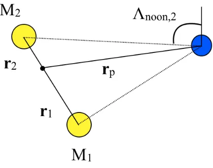
Figure 1: The simulation setup. Stars 1 and 2 orbit the centre of mass with position vectorsr1andr2, and

the planet orbits with position vectorrp. For illustration, the longitude of noon for star 2 is also shown.

and the obliquity of the planet’s rotation relative to the binary orbital plane isδp. At any time during the

simulation, the positions of the stars and planets are given byri(t), wherei = 1,2, p, and the relative

vector

rij=ri−rj (1)

The surface of the planet is divided into cells of longitudeΛand latitudeΦ. We define the longitude of noon

Λnoon,ias the longitude on the planet’s surface at which stariis at its maximum height, wherei= 1,2:

Λnoon,i= tan−1

_r

pi.ˆy

rpi.ˆx

(2)

The planet rotates with a periodPspin, and hence the apparent longitude of a fixed location on the planet

surface (for a given star) varies as

Λs(t) = Λ(t= 0)−Λnoon,i+

2πt

Pspin

(3)

We fixPspin= 24hfor all runs. Resonances between the spin and orbital periods are clearly extremely

influential on the flux distribution, and both the dynamics and habitability of planets in spin-orbit

reso-nances around single stars have been investigated in detail (Dobrovolskis, 2007, 2009; Brown et al., 2014).

However, it is unclear what spin-orbit resonances are available to a circumbinary planetary system, if at all

2.2

Calculating the Received Flux

The Cartesian surface normal vector for a given longitude/latitude cell,ns(Λi(t),Φ), is constructed in the

customary fashion using spherical polar co-ordinates:

ns,x= sin Φ cos Λi

ns,y= sin Φ sin Λi

ns,z= cos Φ

(4)

And then rotated along the x-axis to generate the correct obliquity:

n→Rxn (5)

whereRxis the standard x-axis rotation matrix. The flux from starshitting this latitude/longitude cell is:

Fs=

Ls

4π|rps|

2ˆrps.ns, forˆrps.ns>0 (6)

Ifˆrps.ns ≤ 0, the latitude/longitude cell is facing away from the star, and should therefore be in its nightside. The calculated flux is set to zero if this is the case.

2.3

Calculating Eclipses and Periods of Darkness

The total flux received by a latitude/longitude cell is simply

Ftot(Λ,Φ, t) =F1(Λ,Φ, t) +F2(Λ,Φ, t) (7)

If one star eclipses the other, then the received flux must be modified. If starieclipses starj, then starjhas

its flux reduced by a factorAijwhich is the area of intersection of two circles corresponding to the starsi

andj.

We measure the flux received at every longitude/latitude as a function of time, as well as averaging the

total flux received over the course of the simulation:

¯

F(Λ,Φ) =

R

Ftot(Λ,Φ, t0)dt0

R

dt0 (8)

This integral is evaluated as a sum with dt → ∆t = 30mins. We also integrate the total time spent in darknessDint over the course of the simulation. We define darkness at any latitude/longitude as any

time interval over which neither star is visible (i.e. Ftot(t) = 0). We shall see that this quantity is not as

3

Results

3.1

Kepler-16b

The Kepler-16 system consists of two relatively low-mass stars, of massesM1 = 0.6897M andM2 =

0.2026M, orbiting each other with a semimajor axis ofabin= 0.224AU and eccentricityebin= 0.15944.

These parameters were taken from Doyle et al. (2011), and we use their values for stellar radii and

lumi-nosity also.

Kepler-16b is a0.3MJup exoplanet, with a semi-major axis of 0.7 AU and eccentricity 0.069, with an

orbital inclination within 0.4 deg of the binary plane. Kepler-16 provides an example of a system with two

low mass stars that will eclipse each other on a relatively long timescale (as the orbital period of the binary

is 41 days), and Kepler-16b’s orbit is just outside the habitable zone (Kane & Hinkel, 2013; Haghighipour

& Kaltenegger, 2013; Forgan, 2014). We will therefore replace Kepler-16b with an Earthlike planet to

assess how flux is distributed in this particular scenario.

We also perform runs without the second star, where the planet orbits the primary with the same

param-eters. We will use this data to identify features that are unique to circumbinary systems. We note here that

orbits at the semimajor axis of Kepler-16b are stable only for low eccentricities (see Discussion). Some

of the patterns displayed here are therefore of limited relevance to Kepler-16b in particular, but we can

consider them as indicative of patterns displayed in as yet undiscovered circumbinary planetary systems

where the binary has a relatively small mass ratio, while permitting stable eccentric orbits.

3.1.1 Flux Patterns

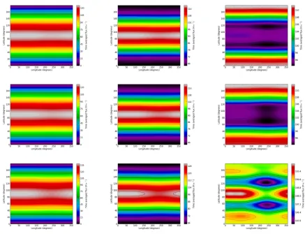
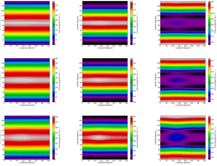
Figure 1 showsF¯on an Earthlike planet with Kepler-16b’s parameters, where we run the simulation for

one orbital period. We fix the planet’s semimajor axis at 0.7 AU, and vary the eccentricity betweenep =

0,0.2,0.5, and the obliquity betweenδp= 0◦,30◦,60◦. The longitudes of periapsis for both the planet and

binary orbits are aligned, which we note will have an affect on resulting surface patterns.

Generally speaking, the features produced by increasing eccentricity are similar to those in the

single-star case: the flux peaks at around the equator, in this case at longitudes around 90◦. However, in the single

star case this peak appears at the substellar point of the planet when it is at periastron. Circumbinary planets

will present two substellar points at periastron - if the obliquity is small, the substellar points both appear

on the equator, at slightly separated longitudes, resulting in the flux being smeared over larger angular area

than in the single-star case.

If the obliquity is high, the flux is more uniformly distributed, as it is in the single star case. However,

the effect of eclipses becomes increasingly important. The orbital period of the planet is around 200 days,

around 5 full orbits of the binary. Therefore, one half of the orbit will experience an extra eclipse period

compared to the other, over the course of an orbital period. At high obliquity, this means one polar region

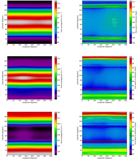
Figure 2: Flux patterns (averaged over the planetary orbital period) for a circumbinary planet in orbit

around the Kepler-16 binary, with withap = 0.7AU, andep = 0(top row),ep = 0.2(middle row) and

ep= 0.5(bottom row). The three columns have obliquitiesδp= 0◦,30◦,60◦respectively.

function of the relative phases of the binary orbit and the planetary orbit - in future years this pattern will

be reversed, and the north will receive more flux than the south.

This may seem surprising initially, as a back-of-the-envelope calculation would suggest that the eclipse

timescale is rather short:

teclipse=

R1+R2 vorbit

≈3 hours, (9)

whereR1 andR2 are the stars’ physical radii, andvorbitis the binary’s orbital velocity. However, this

equation is valid only for a static observer, and the planet moves at its own orbital velocity relative to the

centre of mass of the system. Therefore the eclipse timescale should be written

teclipse=

R1+R2 vorbit,relative

, (10)

0.0

0.2

_{Time (Orbital Period)}

0.4

0.6

0.8

1.0

0

100

200

300

400

500

Flu

x (

W

m

−

2

)

Total

Primary

Secondary

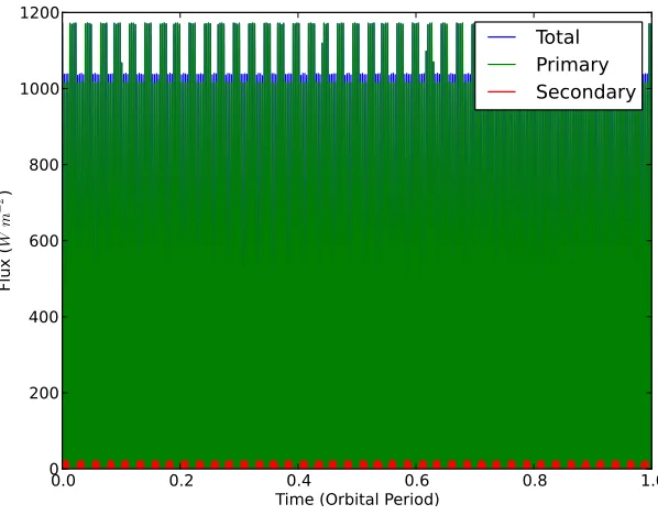
Figure 3: The variation of received flux with time, for a planet orbiting the Kepler-16 binary atap = 0.7

AU, with eccentricityep= 0and obliquityδp= 0◦. The flux is measured at the planet’s equator, along the

prime meridian. Curves are plotted for flux from the primary and secondary, as well as the total received

flux.

rest. Figure 3 shows how the flux in a single longitude/latitude cell varies with time for a planet orbiting

Kepler-16 atap= 0.7AU, with zero eccentricity and obliquity (the flux is measured at the planet’s equator

along the prime meridian).

We can see that the total flux varies according to several distinct timescales. Firstly, there is the standard

day/night cycle, which operates at the highest frequency. As this example has ep = 0, δp = 0◦, this

frequency is fixed. The motions of the binary around the centre of mass add an amplitude modulation to

this signal, with a period equal to the binary’s period. Finally, the effect of eclipses reduces or completely

erases the flux at regular intervals - we can see that the eclipse timescale is indeed much longer than a few

hours. As the secondary has a smaller radius than the primary, the primary is only partially eclipsed by the

secondary, but the secondary is totally eclipsed by the primary.

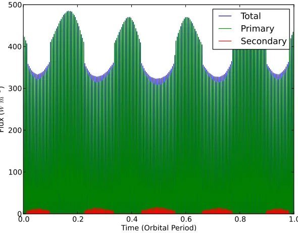
3.1.2 Darkness Patterns

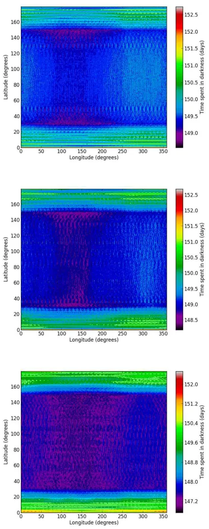
For a planet in a circular orbit around a single star, the total amount of time spent in darkness, for any given

longitude and latitude, will be half of the orbital period1_{. If the planet’s orbit is eccentric, then the changing}

orbital velocity will ensure that for non-zero obliquity, the planet’s northern hemisphere can experience a

longer winter than the southern hemisphere (for example).

If the planet is in a binary system, then for a given location on its surface to be in darkness, both stars

must not be in the sky. Figure 4 shows the total time spent in darkness for planets with obliquityδp= 30◦

orbiting the Kepler-16 binary. We also run (but do not show here) simulations with the secondary removed,

to assess our ability to measure uniform darkness times.

In these single star runs, for circular orbits, the darkness time in the single star case is quite uniform, to

within the numerical limits of the simulation (i.e. for∆t≈30 mins). The range in measured darkness time is a few hours for the circular orbit case (this value is so large due to difficulties measuring the darkness

period at the polar circles of the planet). As the eccentricity increases, it is clear that some longitudes

receive less daylight than others, and this is a function of orbital phase. The limits introduced by a finite

timestep introduces problems resolving along the latitude of the polar circles - however, it is clear that for

a single star system there is no evidence of any latitudinal dependence.

In the twostar case (Figure 4) the difference is stark. The overall time spent in darkness is shorter

-this is a natural consequence of having a second radiation source. However, we can see a clear latitudinal

differentiation, demarcated by the polar circles. These are regions where darkness can occur in protracted,

uninterrupted intervals as well as part of the night/day cycle. As the planet orbits the centre of mass of the

system, the motion of the stars can be sufficient to hide them from view when the higher latitudes would

normally begin their exit from winter, if their radiation source resided at the local centre of mass. This

introduces a slight delay on when daylight returns to these regions, adding extra darkness time. Even in

the case of a circular orbit, the difference in darkness time between the polar and equator regions can be as

large as 8 days!

3.2

Kepler-47c

Kepler-47 is composed of a G star and an M star, with massesM1 = 1.043M andM2 = 0.362M

respectively. Their orbit has semimajor axisabin = 0.0836AU and eccentricityebin = 0.0234. Other

properties are taken from Orosz et al. (2012).

Kepler-47 is the first circumbinary planetary system with multiple planet detections. At an orbital

semimajor axis of 0.989 AU, with an eccentricity constrained to be less than 0.4, Kepler-47c is in the

habitable zone of this system (Kane & Hinkel, 2013; Haghighipour & Kaltenegger, 2013; Forgan, 2014),

whereas Kepler-47b is too close to the binary (and subsequently too hot).

Again, Kepler-47c is not an Earthlike planet, but for our purposes we will assume an Earthlike planet

exists at the same semimajor axis as Kepler-47c. This binary system has a relatively large binary mass

Figure 4: Darkness patterns for (left column) a circumbinary planet in orbit around the Kepler-16 binary,

each withap = 0.7AU, obliquityδp = 30◦, and (top row)ep = 0, (middle row)ep = 0.2, (bottom row)

3.2.1 Flux Patterns

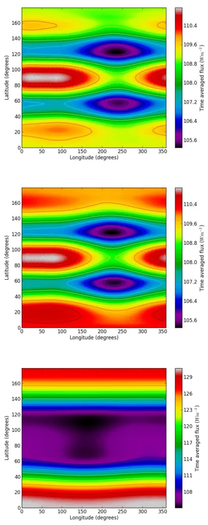
Figure 5 shows the time integrated flux for planets orbiting the Kepler-47c binary atap = 0.989AU. We

again vary the eccentricity betweenep= 0,0.2,0.5(top, middle, bottom rows), and the obliquity between

δp= 0◦,30◦,60◦(left, middle, right columns).

The low obliquity cases are very similar to those for Kepler-16b. Again, the peak flux is spread over a

wider range of longitudes than would be seen for a single star - however, the relatively smallabinplaces

the two substellar points closer together on the planet’s surface, and so the smearing of flux is less evident.

Also, the secondary luminosity is a good deal smaller than the primary luminosity, so it contributes much

less to the total surface flux, relatively speaking.

For high obliquities, we do not see the poles receiving significantly different levels of flux. The eclipse

timescale is significantly smaller than that of Kepler-16b - as a result, for circular orbits the planet will

experience around 40 primary eclipse events per orbit (see Figure 6). Consequently, both the northern and

southern hemispheres will experience very similar numbers of eclipses during their summer periods. Also,

the large mass ratio of the binary ensures that eclipses of the secondary by the primary have an almost

negligible effect on the incoming flux.

Figure 6 demonstrates the minimal effect of the second star on the flux received at a given latitude/longitude.

Eclipses of the primary cause a drop in flux of around 15%, but the event is brief, lasting approximately 3

hours.

3.2.2 Darkness Patterns

Figure 7 shows the time spent in darkness for a planet with obliquityδp = 30◦, orbiting the Kepler-47

binary. Again, we see that the single star case (not shown here) has relatively uniform darkness time. The

simulation timestep is kept the same as for Kepler-16, so with Kepler-47c’s increased orbital period, the

simulation can carry out significantly more timesteps, improving its ability to measure uniform darkness

maps.

A circular, zero obliquity orbit around the Kepler-47 binary has a range in darkness time of around

4 days, increasing to around 5 days as the eccentricity is increased. Again, different darkness regimes

are separated by the polar circles. This is for the same reasons as seen for Kepler-16 - during prolonged

darkness periods in the winter, the orbital motions of the stars introduces a slight delay into the first sunrise

of the spring.

We see a slight longitudinal dependence appearing asep is increased: comparingΛ = 120◦toΛ =

300◦shows a difference in darkness time of around 1 day. This is two to three times larger than the range

seen in single star cases where we expect uniform darkness maps, so we are confident that this effect is not

Figure 5: Flux patterns (averaged over the planetary orbital period) for a circumbinary planet in orbit

around the Kepler-47 binary, withap = 0.989 AU, andep = 0(top row),ep = 0.2(middle row) and

0.0

0.2

_{Time (Orbital Period)}

0.4

0.6

0.8

1.0

0

200

400

600

800

1000

1200

Flu

x (

W

m

−

2

)

Total

Primary

Secondary

Figure 6: The variation of received flux with time, for a planet orbiting the Kepler-47 binary atap= 0.989

AU, with eccentricityep= 0and obliquityδp= 0◦. The flux is measured at the planet’s equator, along the

prime meridian. Curves are plotted for flux from the primary and secondary, as well as the total received

flux.

4

Discussion

4.1

The effect of orbital inclination

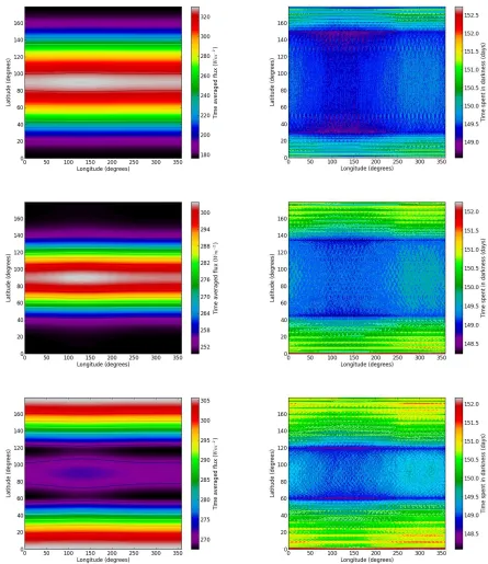
Figure 8 shows dependence of both flux and darkness patterns on orbital inclination for the Kepler-47

system. As abin andebin are both relatively low, the binary sufficiently resembles an extended single

star that increasingip is equivalent to increasingδp, making the flux and darkness patterns difficult to

distinguish from a simulation with high obliquity orbiting in the binary plane (ip= 0).

Kepler-16 presents a larger abin and more equal mass ratio. Figure 9 shows there are some small

differences in the presented flux and darkness features compared to Kepler-47. The flux is distributed over

a larger latitudinal range forip = 15◦, and the eclipse timing effects which gave the south pole more flux

forδp= 60◦,ip= 0◦become apparent again forδp= 30◦,ip = 30◦.

4.2

Sensitivity to the binary orbital phase

Many of the flux patterns we have studied show strong longitudinal dependences, in particular where the

substellar points are during the planet’s periastron passage. AsPorb,binandPorb,pare generally

incommen-surate, we should investigate how the relative orbital phases affect the resulting flux pattern. The simplest

Figure 7: Darkness patterns for a circumbinary planet in orbit around the Kepler-47 binary, each with

Figure 8: The effect of increasing orbital inclination. Flux patterns (left column) and darkness patterns

(right column)for a circumbinary planet in orbit around the Kepler-47 binary with obliquityδp = 30◦,

eccentricityep = 0, and (top row) orbital inclinationip = 0, (middle row)ip = 15◦, and (bottom row)

Figure 9: The effect of increasing orbital inclination. Flux patterns (left column) and darkness patterns

(right column)for a circumbinary planet in orbit around the Kepler-16 binary with obliquityδp = 30◦,

eccentricityep = 0, and (top row) orbital inclinationip = 0, (middle row)ip = 15◦, and (bottom row)

planet periastron occurs att= 0, the relative orbital phase is changed as a result.

Figure 10 displays the flux patterns observed in the Kepler-16 system (forep = 0.5,δp= 60◦), as the

longitude of periapsis is increased. As the relative orbital phase changes, the strong peak in flux at southern

latitudes weakens, and finally disappears. This sensitivity to phase will have important consequences for

fluxes averaged over more than one orbit, as we will see in the following section.

4.3

The persistence of patterns over many orbits

The patterns seen thus far relate to one full orbit of the planet around the centre of mass. As we have seen

that the underlying cause of these patterns are in the relationship between the planet’s orbital phase, the

binary’s orbital phase and their other respective orbital parameters, will such unusual patterns persist over

many orbits, or will they “average out” into a morphology more consistent with a single star system?

Generally speaking, the flux patterns average out to a more uniform distribution, as the difference

between the binary and planet’s orbital longitudes precesses, allowing the stars’ substellar points to move

across all longitudes. The darkness patterns, however, remain distinct. Figure 11 compares the darkness

patterns over 1 planetary orbital period to 100 planetary orbital periods for two cases. The first is the

Kepler-16b system, withep = 0.2 andδp = 30◦; the second is the Kepler-47c system withep = 0.5,

δp= 30◦.

4.4

Orbital Stability, and the potential for spin-orbit resonances

Until now, we have considered circumbinary planets with the same rotation period as the Earth,Pspin = 24

h, but this is clearly not generally true, even for “Earthlike” planets around single stars. As a consequence

of total angular momentum conservation, tidal interactions between a host star and a planet can transfer spin

angular momentum into orbital angular momentum. Typically, the long term tidal evolution of exoplanets

at close distances to their star results in circular orbits with synchronous rotation, wherePspin =Porb,p,

with obliquities generally locked into a Cassini state corresponding either to high or low values (Peale,

1969; Henrard & Murigande, 1987). If the initial orbit is eccentric, the planet can be captured into am:n

spin-orbit resonance, wheremPspin=nPorb,p, withm, nintegers.

Mercury is currently locked in a 3:2 spin orbit resonance with the Sun, thanks to its modest eccentricity

of 0.206. It can be shown that this capture was probable (Correia & Laskar, 2004; Dobrovolskis, 2007),

and stable over long timescales. As such, spin-orbit resonances such as 3:2 may be a common feature of

habitable planets around M stars. As has been previously mentioned, the effects of resonances between

Pspin andPorb,pon flux patterns have been considered in detail for single star systems (Dobrovolskis,

2007, 2009, 2013; Brown et al., 2014).

To date, there has not been any in-depth dynamical study of spin-orbit resonances for circumbinary

Figure 10: The effect of relative orbital phases. Flux patterns for a circumbinary planet in orbit around the

Kepler-16 binary with obliquityδp = 60◦, eccentricityep = 0.5, and (top) longitude of periapsis of0◦,

Figure 11: The persistence of patterns with time. Top row: Darkness patterns for the Kepler-16b system,

withep = 0.2, δp = 30◦. Bottom row: Darkness patterns for the Kepler-47 system, withep = 0.5,

δp= 30◦. The left column displays results from one orbital period of the planet; the right column displays

impact on hazardous flare activity (Mason et al., 2013), but none consider the spin-orbit evolution of the

planet itself. This may be a reasonable lapse, as the calculations for single stars suggest that spin-orbit

evolution such as that seen for Mercury (and proposed for other exoplanets) only occurs ifapis sufficiently

small.

In circumbinary planetary systems, there is a lower limit forap, underneath which planetary orbits are

no longer dynamically stable (Holman & Wiegert, 1999)

ap> adyn=abin 1.6 + 5.1ebin+ 4.12µbin−2.22e2bin−4.27µbinebin−5.09µ2bin+ 4.61µ

2 bine 2 bin , (11)

whereµbin = _MM2

1+M2. The Kepler-47 system can be thought of as a solar-type system perturbed by the

presence of the M type companion, so it may be reasonable to assume that tidal interaction calculations

made for the Solar System, while inaccurate for this case, will give a sense of broad trends. In the absence

of a detailed calculation of the combined tidal interaction between both stars and any planet in the system,

we can compareadynto the orbital semimajor axis of Mercury, which is 0.381 AU, and consider whether

in the first instance Mercury’s orbit would be stable, and leave the details of the interaction to later work. In

the case of Kepler-47,adyn= 0.202AU, so without the benefit of detailed calculation, we should consider

the possibility that some planets could enter a spin-orbit resonance. However, as in the case of the Solar

System, it is likely that planets susceptible to spin-orbit resonances in the Kepler-47 system would also lie

outside the habitable zone.

For Kepler-16,adyn= 0.645AU, and most authors agree this means most of, if not all, of its habitable

zone is orbitally unstable (Liu, Zhang & Zhou, 2013). As we have already stated, eccentric orbits in

the Kepler-16 system with Kepler-16b’s semimajor axis are not stable, which we confirm via N-Body

simulation (Figure 12). Given the low mass of both stars, it seems that planets cannot orbit sufficiently

close to the binary to undergo significant tidal interactions, but once again we stress that this is at best an

educated guess, and requires further work.

We should also note that circumbinary planets generally display rapid apsidal precession, behaviour

that is confirmed both analytically and by N-Body simulation by other authors (Doyle et al., 2011; Orosz

et al., 2012; Leung & Lee, 2013). This precession will have important consequences for planetary seasons,

and may also produce secular resonances, with corresponding effects on much longer timescales.

4.5

Prospects for photosynthesis

It seems clear that the patterns of both flux and darkness measured in this work could lead to patterns

of rhythmicity that are unusual on the Earth (although we can appeal to some terrestrial analogues). The

changing spectral quality reaching the planetary surface caused by the changing dominance of the radiation

0.6 0.8 1 1.2 1.4 1.6

0 10 20 30 40 50

a/AU

t/years

e = 0.0 e = 0.2 e = 0.5

0 0.2 0.4 0.6 0.8 1

0 10 20 30 40 50

e

t/years

e = 0.0 e = 0.2 e = 0.5

Figure 12: Orbital stability of planets orbiting the Kepler-16 binary under N-Body integration. We show

the semimajor axis (left), and eccentricity (right) for planets with initial eccentricities of 0 (red), 0.2 (green)

and 0.5 (blue). Thee= 0.5planet is ejected from the system after∼2 years, whereas thee= 0.2planet is ejected after several hundred years.

specialise in using particular regions of the spectrum, particularly as it shifts from short to longer

wave-lengths.

This spectral niche differentiation is seen on the Earth, across scales similar to that observed at different

depths in the Earths oceans (Stomp et al., 2007; Raven, 2007). O’Malley-James et al. (2012) considered

photosynthesis on an Earth-like planet orbiting in the habitable zone of a close binary system comprising a

G and an M star. That paper emphasises the possibility of a greater significance of photosynthetic organisms

using radiation at wavelengths out to about 1000 nm than is the case on Earth, although the radiation

environment of the Earth-like planet orbiting a G-M binary is dominated by the G star. Figure 13 shows the

spectral flux density reaching the surface of a planet in the Kepler-16 system, orbiting at zero eccentricity

and zero obliquity. In the left plot, the primary is close to its maximum altitude in the sky (primary midday),

and in the right plot it is close to the horizon (primary sunset). Note that the secondary flux is increasing

as the primary flux is decreasing, and exceeds the primary flux at infrared wavelengths during and after

primary sunset. The effects of such changes in infrared flux on photosynthesis depends on the extent

to which global photosynthesis depends on photon absorption in the 700-1000 nm range; this is in turn a

function of the global occurrence of infrared-absorbers and the depth of infrared-absorbing water overlying

them (Wolstencroft & Raven, 2002; Stomp et al., 2007; O’Malley-James et al., 2012).

The changing intensity of light and darkness on the planets discussed is analogous to the onset of

lunar day, in which an additional light cycle with a lower frequency is superposed on the diurnal day/night

cycle. On Earth, it has been found that animals can synchronise their activities to a great diversity of

natural, geophysical rhythms, for example diurnal (24 hours), tidal (12.4 hours), semilunar (14.8 days),

lunar (29.5 days), annual, seasonal, or photoperiodic (365 days), as well as longer cycles involving prime

200 300 400 500 600 700 800 900 1000 Wavelength (nm) 10-10 10-9 10-8 10-7 10-6 10-5 10-4 10-3 10-2 10-1 100 101 Sp ec tra l F lux De nsi ty ( W m − 2nm − 1) Primary Secondary

200 300 400 500 600 700 800 900 1000

Wavelength (nm) 10-10 10-9 10-8 10-7 10-6 10-5 10-4 10-3 10-2 10-1 100 101 Sp ec tra l F lux De nsi ty ( W m − 2nm − 1) Primary Secondary

Figure 13: Spectral variation over the course of a (primary) day in the Kepler-16 system. The left hand plot

shows the spectral flux density when the primary is at maximum altitude (i.e. midday), and the right hand

plot shows the same for when the primary is setting.

et al., 2013). There is an evolutionary advantage of responding to stimuli which correlate with recurring

environmental conditions. The lunar cycle is known to cause an enormous number of biological responses

(Endres & Schad, 2002), for example the timing of breeding in marine organisms. This is despite the

moon being relatively faint (some 400,000 times fainter than the Sun in the optical). It is true that some of

these biological cycles are driven by tides, but we argue that biological rhythms driven by light cycles are

likely to be present in organism behaviour of inhabited circumbinary planets, especially as the secondary

light source is significantly brighter. Given that the periodicity of light cycles in circumbinary systems

can be both greater than and less than the planet’s rotational period, we should expect that in biospheres

of circumbinary planets, selection pressures will exist for biological cycles tuned to a variety of different

rhythms, with the principal cycles linked to the period of the binary.

5

Conclusions

We have calculated time-dependent surface maps of both flux and darkness on planets in circumbinary

systems. Using Kepler-16 and Kepler-47 as archetypes, we model the flux arriving from both stars as a

function of planet latitude and longitude, given an initial Keplerian orbit with fixed elements, and a fixed

spin obliquity.

We identify patterns in both the flux and darkness that are unique to binary star systems. These patterns

exist as both changing spatial distributions and temporal fluctuations. The spectral quality of radiation that

might be considered photosynthetically useful also varies with time and surface position. All the above

variations have periods, amplitudes and phases that depend on the relative orbital phase between the stellar

orbit and the planetary orbit, with timescales both much larger than the planetary orbital period and much

It is clear that if climate modelling of Earthlike circumbinary planets is to go beyond simple 1D

ap-proximations (Forgan, 2014) towards more sophisticated 3D global circulation models (e.g. Shields et al.

2014; Yang et al. 2014) then these surface flux and darkness patterns will play a crucial role in determining

both atmospheric physics and oceanic circulation (and the subsequent interactions thereof).

With such a wide variety of forcing timescales for photosynthesis, we conclude that any inhabited

circumbinary planet will produce a biosphere rich in rhythms and cycles, determined by non-trivial

rela-tionships between the planet’s orbit, the binary orbit, and the location of biomes on the planetary surface.

Acknowledgments

DF and CC gratefully acknowledge support from STFC grant ST/J001422/1. AM acknowledges the

sup-port of a STFC studentship. The University of Edinburgh is a charitable body, registered in Scotland, with

registration number SC005336. The University of Dundee is a charitable body registered in Scotland, with

registration number SC 15096.

References

Brandt T. D., Spiegel D. S., 2014, eprint arXiv:1404.5337

Brown S. P., Mead A. J., Forgan D. H., Raven J. A., Cockell C. S., 2014, International Journal of

Astrobi-ology, in press

Correia A. C. M., Laskar J., 2004, Nature, 429, 848

Cuntz M., 2014, ApJ, 780, 14

Dobrovolskis A. R., 2007, Icarus, 192, 1

Dobrovolskis A. R., 2009, Icarus, 204, 1

Dobrovolskis A. R., 2013, Icarus, 226, 760

Doyle L. R. et al., 2011, Science (New York, N.Y.), 333, 1602

Dressing C. D., Charbonneau D., 2013, ApJ, 767, 95

Endres K.-P., Schad W., 2002, Moon Rhythms in Nature: How Lunar Cycles Affect Living Organisms.

Floris Books, Edinburgh

Forgan D., 2014, MNRAS, 437, 1352

Forgan D., Yotov V., 2014, MNRAS, 441, 3513

Haghighipour N., Kaltenegger L., 2013, ApJ, 777, 166

Hart M. H., 1979, Icarus, 37, 351

Heller R., Zuluaga J. I., 2013, ApJ, 776, L33

Henrard J., Murigande C., 1987, Celestial Mechanics, 40, 345

Hinkel N. R., Kane S. R., 2013, ApJ, 774, 27

Holman M. J., Wiegert P. A., 1999, Astronomical Journal, 117, 621

Huang S.-S., 1959, PASP, 71, 421

Kaltenegger L., Sasselov D., 2011, ApJ, 736, L25

Kane S. R., Ciardi D. R., Gelino D. M., von Braun K., 2012, MNRAS, 425, 757

Kane S. R., Gelino D. M., 2012, Astrobiology, 12, 940

Kane S. R., Hinkel N. R., 2013, ApJ, 762, 7

Kasting J., Whitmire D., Reynolds R., 1993, Icarus, 101, 108

Kasting J. F., Kopparapu R., Ramirez R. R., Harman C., 2013, PNAS, in press

Kipping D. M., Forgan D., Hartman J., Nesvorn´y D., Bakos G. A., Schmitt A., Buchhave L., 2013, ApJ,

777, 134

Kopparapu R. K. et al., 2013, ApJ, 765, 131

Kopparapu ., Ramirez ., SchottelKotte ., Kasting ., Domagal-Goldman ., Eymet ., 2014, eprint

arXiv:1404.5292

Leung G. C. K., Lee M. H., 2013, ApJ, 763, 107

Liu H.-G., Zhang H., Zhou J.-L., 2013, ApJ, 767, L38

Livengood T. A. et al., 2011, Astrobiology, 11, 907

Mason P. a., Zuluaga J. I., Clark J. M., Cuartas-Restrepo P. a., 2013, ApJ, 774, L26

Mayor M., Queloz D., 1995, Nature, 378, 355

O’Malley-James J. T., Raven J. A., Cockell C. S., Greaves J. S., 2012, Astrobiology, 12, 115

Peale S. J., 1969, The Astronomical Journal, 74, 483

Petigura E. A., Howard A. W., Marcy G. W., 2013, Proceedings of the National Academy of Sciences of

the United States of America, 110, 19273

Quarles B., Musielak Z. E., Cuntz M., 2012, ApJ, 750, 14

Raven J., 2007, Nature, 448, 418

Raven J. A., Cockell C. S., 2006, Astrobiology, 6, 668

Rein ., Fujii ., Spiegel ., 2014, eprint arXiv:1404.6531

Seager S., Bains W., Hu R., 2013a, ApJ, 775, 104

Seager S., Bains W., Hu R., 2013b, ApJ, 777, 95

Selsis F., Kasting J. F., Levrard B., Paillet J., Ribas I., Delfosse X., 2007, A&A, 476, 1373

Shields A. L., Bitz C. M., Meadows V. S., Joshi M. M., Robinson T. D., 2014, ApJ, 785, L9

Sota T., Yamamoto S., Cooley J. R., Hill K. B. R., Simon C., Yoshimura J., 2013, Proceedings of the

National Academy of Sciences of the United States of America, 110, 6919

Stomp M., Huisman J., Stal L. J., Matthijs H. C. P., 2007, The ISME journal, 1, 271

Underwood D., Jones B., Sleep P., 2003, International Journal of Astrobiology, 2, 289

Welsh W. F. et al., 2012, Nature, 481, 475

Williams D. M., Pollard D., 2002, International Journal of Astrobiology, 1, 61

Wolstencroft R., Raven J. A., 2002, Icarus, 157, 535