Global behaviour corresponding to the absolute instability of the rotating disc boundary layer

+

University of Warwick institutional repository: http://go.warwick.ac.uk/wrap

This paper is made available online in accordance with

publisher policies. Please scroll down to view the document

itself. Please refer to the repository record for this item and our

policy information available from the repository home page for

further information.

To see the final version of this paper please visit the publisher’s website.

Access to the published version may require a subscription.

Author(s): CHRISTOPHER DAVIES and PETER W. CARPENTER

Article Title: Global behaviour corresponding to the absolute instability of

the rotating-disc boundary layer

Year of publication: 2003

Link to published

DOI: 10.1017/S0022112003004701 Printed in the United Kingdom

287

Global behaviour corresponding to the absolute

instability of the rotating-disc boundary layer

By C H R I S T O P H E R D A V I E S1 _{A N D P E T E R W. C A R P E N T E R}2 1_{School of Mathematics, Cardiff University, Cardiff, CF24 4YH, UK}

2_{School of Engineering, University of Warwick, Coventry, CV4 7AL, UK}

(Received6 April 2001 and in revised form 3 March 2003)

1. Introduction

For more than fifty years the rotating disc has been the model flow for studying three-dimensional boundary-layer instability and transition. During this period many papers have appeared describing theoretical and experimental research on this topic. One might have been forgiven, then, for assuming that the major features of instability and transition had already been discovered for this model flow and that only rather academic and arcane points remained to be elucidated. This view was to be dispelled by the revelation of Lingwood (1995) that the rotating-disc flow is absolutely unstable. Furthermore, the theoretical critical Reynolds number for absolute instability is more or less coincident with the experimentally observed transition point. A little later Lingwood (1996) also described an experimental investigation which appeared to corroborate her earlier theoretical study.

Absolute instability is a local concept in that it is defined theoretically by a stability analysis of the local velocity profiles. In effect, such an analysis assumes a spatially homogeneous flow. This is often termed theparallel-flowapproximation. However, this term is, perhaps, not entirely appropriate for the rotating-disc flow as the boundary layer remains at constant thickness throughout. For this flow it is the increase in the magnitude of the undisturbed velocity field proportionately to radius that is responsible for the spatial inhomogeneity. In the present paper we investigate how spatial inhomogeneity affects the global response of this locally absolutely unstable flow. The study is based on direct numerical simulations of the complete linearized Navier–Stokes equations, obtained with the novel velocity–vorticity method presented in Davies & Carpenter (2001, hereafter referred to as I).

It is important to emphasize that our numerical simulations are not equivalent to an instability analysis. In fact, they have more in common with physical experiments than stability theory. Beyond omitting the nonlinear terms in the form of the Navier– Stokes equations governing the perturbation flow field, the form of the perturba-tions in our simulaperturba-tions is not specified in any way. Just like a physical experiment the perturbations are initially excited by a local time-dependent displacement of the disc surface. The subsequent evolution of the disturbance is governed purely by the (linearized) Navier–Stokes equations. Accordingly, there is no need to evoke causality as in instability analysis, any more than one would need to do so for a physical experiment. Indeed, it would be inappropriate to attempt to do so.

Ours appears to be the first study of the global behaviour corresponding to the absolute instability of the rotating-disc boundary layer,† although, of course, Lingwood’s experimental investigation is perforce also a study of the global behaviour. Previous numerical studies of the rotating-disc flow that took account of the inhomogeneous radial variation either did not reveal any vestige of absolute instability (Spalart 1991), or were based on the parabolic-stability-equation (PSE) approach (Malik & Balakumar 1992) and therefore not able to accommodate the upstream propagation of disturbances.

Lingwood’s discovery of the absolute instability was completely novel and came as a surprise to the research community. Nevertheless, as she herself pointed out, there were clues to be found in the previous experimental studies. (We will not attempt to review the relevant literature here, but instead refer the reader to the reviews by Reed & Saric (1989) and Saric, Reed & White (2003) and the introduction in Cooper &

Carpenter (1997a).) For example, in the surface flow visualizations of Gregory, Stuart & Walker (1955), using the china-clay technique, the transitional radius is very sharp. More recent flow visualizations (e.g. Kobayashi, Kohama & Takamadate 1980) also exhibit the same feature. The sharpness of the transition line on the rotating disc contrasts markedly with those normally found when boundary-layer transition is due to the amplification of convective instabilities like Tollmien–Schlichting waves. In these cases one typically sees wedges of turbulent flow upstream of the main transition line that are created by local roughness formed by the pigment or tracer particles used for the flow visualization. Lingwood (1995) also pointed out that the values of transitional Reynolds number measured in the many experimental studies of the rotating-disc flow differed by less than 3% from the average value of about 513. Again, this is in sharp contrast with transition in flows dominated by convective instabilities, such as pipe flow or boundary layers over flat plates. In the latter case, for example, the transitional Reynolds number is very sensitive to background noise and environmental factors; consequently, transitional Reynolds numbers ranging from 100 000 to in excess of 2×106 _{have been reported in the literature (Schlichting 1979).}

Theoretical evidence pointing to the possibility of absolute instability was also available in the literature. First, as pointed out by Lingwood (1995), the velocity profiles for the rotating-disc boundary layer exhibit reverse flow when resolved in a range of directions between the radial and azimuthal directions. Since absolute instability requires upstream propagation, and a reverse undisturbed flow facilitates upstream propagation, it is found in many examples of absolutely unstable flow. Examples are given by Huerre & Monkewitz (1990). These include countercurrent mixing layers in circular jets (Strykowski & Niccum 1991), and the wakes behind circular cylinders (Mathis, Provansal & Boyer 1984; Koch 1985; Triantafyllou, Triantafyllou & Chryssostomidis 1986; Monkewitz 1988; Strykowski & Sreenivasan 1990), blunt bodies (Hannemann & Oertel 1989; Oertel 1990) and a floating cylinder (Triantafyllou & Dimas 1989). But reverse flow certainly does not guarantee absolute instability, nor is it always necessary.

result is an algebraically growing disturbance rather than an absolute instability. This phenomenon was investigated in I and also in a recent paper by Turkyilmazoglu & Gajjar (2000).

Huerre & Monkewitz (1990) give an excellent review of the global instability of spatially developing flows, especially its relationship to absolute instability. Accordingly, we will largely confine ourselves to reviewing the developments since 1990 that are relevant to our study. The concepts of absolute and convective instability are strictly only valid for a spatially homogeneous flow. They are extended to spatially developing flows by making a so-called quasi-parallel-flow approximation whereby one examines the stability of a model spatially homogeneous flow having the same streamwise velocity profile as the real spatially inhomogeneous flow at the selected spatial location. Thus a dispersion relation

D(α, ω;R) = 0 (1)

can be formulated linking the complex frequency and wavenumber at a given value of R where α and ω are the non-dimensional wavenumber and frequency. R is the Reynolds number based on the local spatial coordinate or variables. For example, for the rotating disc

R= _√rr∗

ν/Ω,

where r_r∗ is the radial location where the stability analysis is carried out, ν is the kinematic viscosity, and Ω the rotational speed of the disc. Thus the coordinate at a fixed radial position is made dimensionless with reference to the constant boundary-layer displacement thickness. The same length scale is also used to make the wavenumber dimensionless and the reference time, 1/(ΩR), is used to make frequency dimensionless.

Purely in the context of boundary-layer instability over the rotating disc, the following remarks can be made about the use of (1). In the approach taken in classic linear instability theory one solves (1) for complex ω, specifying α and keeping it real. Convective instability is then indicated when ωi > 0 for a given combination of αr and R. Gaster (1962, 1965) showed that spatially growing waves are a better representation of convectively unstable disturbances seen in most physical applications and experiments. In this case, ω is specified and kept real, and (1) is then solved for complex α, and −αi>0 marks the onset of convective instability for a given combination of ωr and R. A Gaster (1962, 1965) transformation can be used to obtain an approximate relationship between the temporal and spatial growth rates, namely

−αi

ωi

cg

, (2)

0

t

x

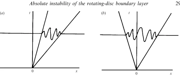
(a) (b) t

0 x

Figure 1. Schematic sketches of the evolution of a wavepacket generated by an impulse.

(a) Convective instability. (b) Absolute instability.

relation (1), and use it to investigate the nature of the Green’s function corresponding to the response of the flow to an impulse. Absolute instability is then indicated by the existence of a pinch-point in the complex α-plane, as originally demonstrated by Briggs (1964) (see Huerre & Monkewitz 1990; Lingwood 1995, 1997a). The value of ωi corresponding to the pinch-point gives the non-dimensional absolute temporal growth rate,ωa,i.

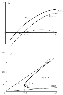
In figure 2(a), we depict the characteristics of the convective and absolute instabilities for the rotating-disc flow. In this case both absolute and convective instability set in at distinct spatial locations. Formally the flow remains unstable for all R > Rc (the critical Reynolds number for the onset of convective instability). According to Lingwood (1995, 1997b) the critical value of the Reynolds number for convective instability is about 290 and that for absolute instability is Ra= 507.3 (corrected in Lingwood 1997b from the value of 510.6 given in Lingwood 1995). Furthermore, as shown in figure 2(a), the maximum values of both ωi and ωa,i are their asymptotic values as R → ∞. The asymptotic value of (ωa,i)max given in figure 2(a) is taken from Lingwood (1995). This apparently distinguishes it from the flows studied and reviewed by Huerre & Monkewitz (1990) for which the maximum absolute growth rate occurred at finite values of R. For the rotating disc, one should include the real azimuthal wavenumber, β, as a parameter in (1) as well as R. For this reason the dependence of the region of absolute instability on both R and β is sketched schematically in figure 2(b). Figure 2(b) also plots the asymptotic absolute stability boundaries. The value for the upper branch, namely β = 0.265R, was given by the inviscid analysis of Lingwood (1995), whereas the lower branch,β= 0.026R is given by the recent analysis of Peake & Garrett (2003). Plainly, for a givenR the flow is only absolutely unstable for a range of values of β. (It should be noted that, in fact, only integer values of β are physically admissible; but for simplicityβ is shown as continuously varying in figure 2b.)

(a)

(b)

ωi

0

507.3

(ω_i) _max (ωa,i) max

0.0133

R

400

200

67

0 507.3 R

β

(ω_a,_i) > 0

7

× 2+

+ +×

3 +5 ₊

1

0.026R 0.265

R

–

4 6

Figure 2.Schematic sketch depicting the characteristics of the local instability of the

rotating-disc boundary layer. (a) Maximum growth rates vs.R; - - -, growth rate for fixedβ. (b) Neutral curve defining the region of absolute instability; the labelled data points denote the conditions for the various numerical simulations presented in§3.

plotted in figure 2(a). Note that this curve is schematic only and does not provide a reliable guide to the magnitude of the maximum growth rate nor to the relative extent of the absolutely unstable region. Some idea of this can be deduced from the lower asymptote β = 0.026R plotted in figure 2(b). From this we estimate that the abso-lutely unstable regime for the critical azimuthal wave-number, β = 67, extends to

R2600.

a slight degree of wall compliance is required to push the absolute instability much further outboard or to eliminate it entirely. Thus by making the disc surface compliant beginning at a radial location well into the absolutely unstable region, we can obtain a flow that is absolutely unstable in a relatively small finite region.

It was our intention at the outset of our study to address three key questions. First, is the existence of the semi-infinite region of absolute instability depicted in figure 2 associated with an amplified linear global response such that a typical flow variable

A∼e−iωGt ₍₃₎

(whereωG=ωG,r+ iωG,iis complex andωG,i >0)? Secondly, if it is, what is the value ofωGand how is it determined? Lastly, in the case with a partially compliant surface, how large does the region of absolute instability need to be to elicit a linear global response of the form (3)? We investigated these questions by means of a numerical simulation of the complete, linearized, Navier–Stokes equations.

What guidance for investigating these questions do previous theoretical studies offer? The forced linearized Ginzburg–Landau equation, namely

∂A ∂t +U

∂A

∂x =µA+γ ∂2A

∂x2 +H(t)F(t)δ(x), (4)

is one of the simplest systems that exhibits absolute instability. Here the system is forced at the pointx= 0 and the time variation of the forcing such that it is ‘switched on’ at t = 0. The global instability of this equation with spatially inhomogeneous coefficients has been investigated by various authors. In such cases, for the purposes of theory the ‘slow’ spatial variable,X=x(whereis a small parameter, typically 1/R) in a WKBJ approximation is regarded as complex. For example, Chomaz, Huerre & Redekopp (1988) investigated the case of linearly varying µ = µ0 +µ1x (where µ1 < 0). They established fundamental results that are central to the questions of

how the existence of global modes and the selection of their complex frequency are connected to the local instability behaviour corresponding to µ= µ0 = const. (See

also Huerre & Monkewitz 1990.) They examined the global behaviour for fixedµ1 as µ0 was increased from an initially negative value. Absolute instability occurs when µ0exceeds the critical valueµa. But it was necessary forµ0to exceedµG> µa before the system became globally unstable. In other words the region of local absolute instability had to reach a certain threshold size before global instability ensued. (See, also, the WKBJ global stability analysis of the vorticity transport equation for non-parallel shear flow by Monkewitz, Huerre & Chomaz 1993.) On the question of how the global frequency is selected, Huerre & Monkewitz (1990) proved that ωG corresponded to the frequency ωa(Xs) of the absolutely unstable local mode located at a saddle point Xs in complex X-space. This selection principle differs from early suggestions made by Pierrehumbert (1984), Koch (1985) and Monkewitz & Nguyen (1987). It follows from the Huerre–Monkewitz selection principle that the global growth rate satisfies the following inequality:

ωG,iωa,i(Xs)6(ωa,i)max. (5)

In the case of the rotating disc, the fact that∂(ωa,i)max/∂R→0 as R→ ∞ might seem to suggest that the equivalent of the saddle point Xs used to determine the complex global frequency by Huerre & Monkewitz is located at R = ∞. If this were so, then the Huerre–Monkewitz approach would be ill-posed in the case of the rotating disc. However, as pointed out above, for fixed β the absolutely unstable region is finite in extent. This suggests that the saddle point is located at a finite value ofR. Very recently, Peake & Garrett (2003) have carried out an inviscid analysis of the global linear stability of the rotating-disc flow that shows the saddle point occurs at a finite value ofR.

There have also been some experimental studies and numerical simulations of global instability. On the whole these are in accordance with the theoretical picture emerging from the studies of the Ginzburg–Landau equation. Most notable are the various experimental and numerical studies of the cylinder wake, reviewed by Huerre & Monkewitz (1990) and briefly discussed above. The global instability of other wake flows has also been investigated by numerical simulation, e.g. the wakes behind blunt bodies (Hannemann & Oertel 1989; Oertel 1990), shallow-water flow past bottom topography in the form of a circular bump (Sch¨ar & Smith 1993), and the wake of a triangular cylinder (Zielinska & Westfreid 1995). Certain jet and plume flows have also been found to exhibit global instability, e.g. hot jets (as reviewed by Huerre & Monkewitz 1990), dripping taps (again, as reviewed by Huerre & Monkewitz 1990, see also Le Diz`es 1997), and, more recently, the flickering candle (Maxworthy 1999) and the plane wake flow with base suction (Leu & Ho 2000). This last paper illustrates well how global instability can be eliminated by shrinking the region of absolute instability, here done by the application of base suction, which eliminates the global instability, even though it causes (ωa,i)max to rise steeply. Moreover the level of base suction required to suppress the global instability is reasonably well predicted by the application of the WKBJ theory of Monkewitzet al.(1993).

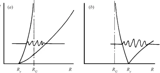
t

R_e R_G R

(a)

R_e

R_G R

(b)

Figure 3. Typical wavepacket evolution for the rotating-disc boundary layer according to

Lingwood’s conjecture. Impulsive excitation (a) at Re < Ra < RG (based on figure 1c of Lingwood 1996); and (b) atRe> RG> Ra.

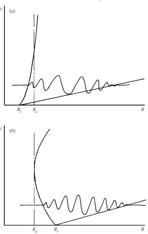
nonlinear effects (e.g. Hannemann & Oertel 1989; Zielinska & Westfreid 1995; Pier & Huerre 1996) suggests that the form of the linear global mode is qualitatively preserved, with nonlinear effects leading to saturation and in some cases causing the global frequency to rise slightly. The exception to this is the steep nonlinear global mode discovered by Pier et al. (1998) which may be more relevant in the present case.

t

R_e R_a R

(a)

t

R_a R_e R

(b)

Figure 4.Schematic sketches of typical wavepacket evolution for the rotating-disc boundary

layer as revealed by our numerical simulations. Impulsive excitation (a) at Re < Ra; and (b) atRe > Ra.

For the rotating disc the upstream convective behaviour appears to be so strong that it dominates the extensive downstream region of absolute instability.

Our results do not seem to conform with the previous work on the global behaviour associated with absolute instability. Evidence from two recent sources, however, strongly suggests that the global response found in our study is not anomalous. First, Monkewitz (2001, personal communication) points out that the behaviour depicted in figure 4(b), whereby the trailing edge of the evolving wavepacket turns back on itself, can be reproduced qualitatively by the linearized Ginzburg–Landau equation (4). All that is required is for the growth rate in (4) to vary asµ=µ0+µ1Xwith complex

coefficients such that Re(µ1)>0. This corresponds qualitatively, more or less, with the

the reason why this behaviour only occurs for complex µ1 in the Ginzburg–Landau

model is intuitively understandable, since the downstream edge reaches more and more ‘oscillators’ at frequencies that are increasingly different (without bound) from the absolute frequency at any given spatial location.

The other recent evidence that supports the results of our study is due to Peake & Garrett (2003). They carried out a global, linear, inviscid, stability analysis of the boundary layer on rotating bodies including the rotating disc as a special case. They find the saddle point that plays a crucial role in the Huerre–Monkewitz approach is located at a finite (complex) value of non-dimensional radius. And, even more significantly, they find that the linear global mode is damped, in agreement with the results of our numerical-simulation study. These results may not be in conflict with the inequality (5) and other principles laid out by Huerre & Monkewitz (1990) and subsequent workers. It is just that for the rotating disc even a semi-infinite region (finite, but extensive, for fixedβ) of absolute instability is insufficient for an amplified global response.

The remainder of the paper is set out as follows. The theoretical and numerical approach has been presented in detail in I, so only fairly brief descriptions are given in §2. Section 3 is the main section of the paper. Here we present the results of our numerical-simulation study of the global behaviour of impulsively generated disturbances in the boundary layer of a rigid rotating disc. We study both cases which are convectively unstable in the equivalent spatially homogeneous flow and those that are absolutely unstable. In §4 we investigate the effects of replacing part of the rigid disc in the absolutely unstable region with a compliant annulus. Finally, conclusions are given in§5.

2. Theoretical and numerical approach

The theoretical and numerical approach is fully described in I. Accordingly, only an outline will be given here.

For the rotating disc the dimensional flow field is defined with respect to a cylindrical coordinate system (r∗, θ, z∗) that is fixed relative to the disc which rotates at speed Ω. The asterisks denote dimensional length coordinates. The undisturbed flow field in this coordinate system is given by the dimensional velocity vector

U∗= (U_r∗, U_θ∗, W). (6)

These velocity components are related to the von K ´arm ´an (1921) similarity solution (F(z), G(z), H(z)) (where z=z∗√Ω/ν and ν is the kinematic viscosity of the fluid) for the rotating-disc boundary layer as follows:

Ur∗=r∗ΩF(z), Uθ∗=r∗ΩG(z), W= √

νΩH(z). (7)

Thus the boundary-layer displacement thickness,δ∗= (ν/Ω)1/2_{, is used as the reference}

length scale for non-dimensionalization; but we also introduce another length scale, namely rr∗ – a reference value of the radial coordinate. Thus r=r∗/δ∗ and the Reynolds number is defined as R=r_r∗/δ∗; r_r∗Ω is used as the reference velocity, 1/(RΩ) as reference time, RΩ as the reference vorticity andρr∗2

Perturbations to the velocity and vorticity fields are introduced that in non-dimensional form are denoted by

u= (ur, uθ, w), ω= (ωr, ωθ, ωz). (8)

It was shown in I that, subject to rather general conditions as z → ∞ that are definitely satisfied in the present case, the Navier–Stokes equations are fully equivalent the following system of governing equations for the primary variables (ωr, ωθ, w):

∂ωr ∂t + 1 r ∂Nr ∂θ − ∂Nθ ∂z − 2 R

ωθ+

∂w ∂r = 1 R

∇2₋ 1 r2

ωr − 2 r2 ∂ωθ ∂θ , (9) ∂ωθ ∂t + ∂Nr ∂z − ∂Nz ∂r + 2 R

ωr− 1 r ∂w ∂θ = 1 R

∇2₋ 1 r2

ωθ+ 2 r2 ∂ωr ∂θ , (10) ∇2 w=1

r

∂ωr

∂θ − ∂(rωθ)

∂r

. (11)

where

N= (Nr, Nθ, Nz) = (∇×U)×u+ω×U+ω ×u

nl

. (12)

The secondary variables are defined in terms of the primary ones as follows:

ur= − ∞

z

ωθ+

∂w ∂r

dz, (13)

uθ= ∞

z

ωr− 1 r

∂w ∂θ

dz, (14)

ωz= 1 r

∞

z

∂(rωr)

∂r + ∂ωθ

∂θ

dz. (15)

Only the perturbations are to be determined in the numerical simulation. In the present study we are only interested in disturbances with vanishingly small amplitude, so we linearize the governing equations by simply omitting the term labelled nl in (12). The resulting system of equations is fully equivalent to the complete linearized Navier–Stokes equations. The linearization permits the boundary conditions at the wall to be simplified in the case when the wall moves in the vertical direction. Vertical displacement of the wall occurs when the wall is compliant and also in the vicinity of the perturbation exciter or driver. The linearized no-slip conditions and the wall-normal zero-displacement conditions become

ur= −

r

RF (0)η, uθ= − r

RG(0)η, w= ∂η

∂t at z= 0, (16a, b, c) where η is the non-dimensional vertical wall displacement. The wall displacement equals zero for a rigid wall. Otherwise it is either specified, as in the case of the driver, or governed by the equation of motion for the compliant wall (see I). Substituting (16a) and (16b) into the definitions (13) and (14) for the secondary variables gives the following integral constraints on the primary variables which replace the no-slip conditions (16a) and (16b):

∞

0

ωθdz=

r

RF(0)η− ∞

0 ∂w

∞

0

ωrdz= −

r

RG(0)η+ ∞

0

1 r

∂w

∂θ dz. (18)

Equation (16c) in its original form as a boundary condition acts as the third constraint on a primary variable.

Linearization makes the problem separable with respect to the azimuthal coordinate θ, which is particularly convenient given our use of a Fourier spectral representation to discretize the azimuthal variation. Thus any given perturbation can be represented as a linear superposition of independent azimuthal modes. We can therefore independently calculate individual azimuthal modes of the perturbation velocity and vorticity fields that take the form

(ur, uθ, w) = ( ˆur,uˆθ,wˆ)einθ, (ωr, ωθ, ωz) = ( ˆωr,ωˆθ,ωˆz)einθ, (19)

where ˆur etc. are functions only of r and z, and n is the integer-valued azimuthal mode number (this notation that recognizes explicitly the integer value replaces β used in§1 where, for convenience, the azimuthal wave-number was regarded as a real number – see figure 2b). The remaining notation is conventional and should be clear. All coordinates and flow quantities are non-dimensional unless specified otherwise. Equation (19) is an inevitable consequence of linearization and not an additional assumption. No other assumptions are made about the form of the perturbations.

As described in I, a fourth-order, centred, compact finite-difference scheme is used for discretization in the r-direction, a Chebyshev spectral scheme used in the wall-normal, i.e.z-direction, and Fourier spectral scheme used in the azimuthal direction. As explained above, for a linear simulation, this form of azimuthal discretization permits us to treat each azimuthal mode independently. Some of the simulations reported below were also repeated using higher-order finite-difference schemes in order to check that the phase errors with the fourth-order scheme were not significant.

3. Numerical simulations for rigid rotating discs

In I we investigated disturbances excited by time-periodic motion of the surface. We now consider the development of disturbances generated by a localized impulsive wall motion. The wall displacementηis taken to be of the form

η(r, θ, t) =a(δr)b(t) einθ, δr =r−re, (20)

with the temporal impulse given by

b(t) = (1−e−σ t2

) e−σ t2

. (21)

Typical forms for the functiona used to localize the forcing motion around a given radiusr =re were described in I. As before, n is the azimuthal mode number. The parameterσ, which fixes the duration of the impulse, was chosen to be large enough for a broad range of temporal frequencies to be incorporated in the excitation. Its magnitude, and hence the highest effective frequency excited, was limited only by the need to retain full temporal resolution of the impulse.

Numerical simulations were conducted first with the fluid governing equations simplified according to the so-called parallel-flow approximation, i.e. the equations

were made spatially homogeneous.† Results from these simulations were found

to conform with the theory of Lingwood (1995). In particular, the existence of absolute instability could be inferred from the temporal behaviour of the simulated disturbances at Reynolds numbers and azimuthal mode numbers lying within the absolutely unstable region determined by Lingwood (see figure 2b). In order to keep our exposition concise, we defer until later any further discussion of the results obtained with the approximate, SH, governing equations. Attention will instead be focused on the behaviour of disturbances that evolve in the real SI boundary layer.

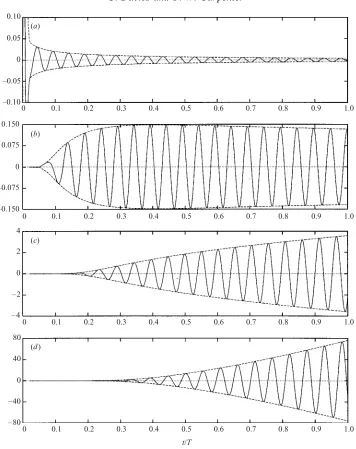
Convective instability

Figure 5 shows time histories, at successive radial locations, for a disturbance with azimuthal mode number n= 32 triggered by an impulse centred at re= 500. (This combination is denoted by Point 1 in figure 2b.) The azimuthal component of the vorticityωθ w at the wall is plotted for a fixed value ofθ, along with the corresponding envelopes ±|ωθ w| obtained from the complex-valued amplitude. (No particular significance should be attached to our repeated selection of ωθ w as a convenient flow-field variable when we discuss the evolution of disturbances. The description of disturbance behaviour, particularly with regard to distinctions between absolute and convective instability, would not need to be altered in any fundamental, qualitative, manner if some other flow-field variable, such as the disturbance energy, were monitored instead of ωθ w. However, as would be expected, the mean-flow SI has the effect of making any calculation of spatial growth rates dependent, to some extent, on the variable selected for measuring the disturbance amplitude. Since we are mostly concerned with detecting the presence or absence of temporal growth, such subtleties need not detain us any further here.)

From figure 5(a), it can be seen that the disturbance decays rapidly atr=re. For

r > re, there is an initial period of quiescence while the disturbance propagates towards the given location and away from its source. As would be expected, the length of this quiescent time interval increases with the radius. When the disturbance eventually

† Hereafter the abbreviations SH and SI will be used respectively forspatially homogeneousand

0.10

0.05

0

–0.05

–0.10

0 0.2 0.4 0.6 0.8 (a)

0 0.2 0.4 0.6 0.8 0.250

0.125

0

–0.125

–0.120

t/T

(c)

0 0.2 0.4 0.6 0.8

0 0.2 0.4 0.6 0.8

t/T

0.050

0.025

0

–0.025

–0.050

(b)

(d) 1.50

0.75

0

–0.75

–1.50

Figure 5. Time histories forω_{θ w} (solid lines), together with corresponding envelopes ±|ω_{θ w}|

(broken lines), for an impulsively excited disturbance. n= 32 and re= 500. (a) r=re= 500, (b)r= 525, (c)r= 550, (d) r= 575.T= 2πR is the non-dimensional time period for the disc rotation.

0.8

0.6

0.4

0.2

475 500 525 550 575 600

t T

r

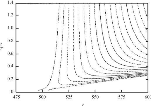
Figure 6. Spatio-temporal development of|ω_{θ w}|for an impulsively excited disturbance with

n= 32. The impulsive disc surface motion used to excite the disturbance was centred atre= 500. (The contours are drawn using a logarithmic scale with levelsA2m_{form= 0,1,2. . ., whereA} is an arbitrary normalization factor.)

0.10

0.05

0

–0.05

–0.10

0 0.1 0.2 0.3 0.4 0.5 0.6 0.7 0.8 0.9 1.0 (a)

0.150

0.075

0

–0.075

–0.150

0 0.1 0.2 0.3 0.4 0.5 0.6 0.7 0.8 0.9 1.0 (b)

(c) 4

2

0

– 2

– 4

0 0.1 0.2 0.3 0.4 0.5 0.6 0.7 0.8 0.9 1.0

0 0.1 0.2 0.3 0.4 0.5 0.6 0.7 0.8 0.9 1.0 80

40

0

– 40

– 80 (d)

t/T

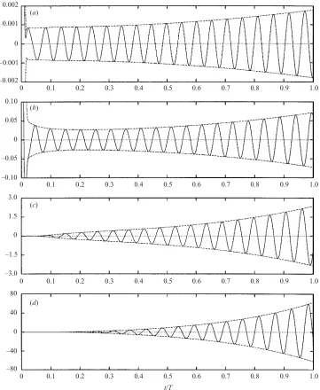
Figure 7.Time histories for ω_{θ w} (solid lines), together with corresponding envelopes±|ω_{θ w}|

(broken lines), for a disturbance with n= 75 that is impulsively excited at re= 500. (a)r=re= 500, (b)r= 525, (c)r= 550, (d)r= 575.

edges of a radially extended disturbance wavepacket. Both ends of the wavepacket propagate outwards with non-zero radial velocities, the leading edge travelling rather more quickly than the trailing edge.

1.4

1.2

1.0

0.8

0.6

0.4

0.2

0

475 500 525 550 575 600

r t

T

Figure 8. Spatio-temporal development of|ω_{θ w}|for an impulsively excited disturbance with

n= 75. The impulsive disc surface motion used to excite the disturbance was centred atre= 500. (Contours drawn using a logarithmic scale, as in figure 6.)

excitation was located atre= 500. (See Point 2 in figure 2b.) It can be seen that the disturbance still decays at r=re, but much less rapidly than for n= 32. At r= 525 there is a period of growth followed by a relatively weak decay. Further out, atr= 550 and r= 575, the disturbance exhibits continuous growth over the whole of the time interval considered. This behaviour provides a marked contrast with the brief growth, followed by decay, exhibited at the corresponding radial positions whenn= 32.

The spatio-temporal development of the disturbance withn= 75 is also displayed in figure 8, using contour plots of|ωθ w|. It may be seen that the leading edge propagates radially outwards with a non-zero velocity comparable to that found when n= 32. However, the trailing edge behaviour is very different than found previously. From a comparison with figure 6, it appears that the trailing edge propagates much more slowly for n= 75 than for n= 32. In fact, the contour plots suggest that the radial velocity of the trailing edge may be approaching zero as the disturbance develops. Such behaviour would be expected if the disturbance exhibited persistent temporal growth at sufficiently large radii. Examination of the numerical simulation data confirmed that, for the time interval of the simulation, there was continual growth for all radial positions beyond r 535. This result may be checked by undertaking a graphical analysis of the contours displayed in figure 8. Locations where there is temporal growth can be determined from the intersections between the contours and vertical lines drawn at each selected radial position.

A more detailed examination of the simulation data plotted in figure 8 revealed that the temporal growth of the disturbance at any fixed radial position was much weaker than the convective growth occurring along the trajectory of the maximum of the wavepacket amplitude. For instance, at r= 550 the disturbance amplitude, as measured by ωθ w, grows by a factorO(23) between t= 0.2T and t= 0.4T, where

800 750 700 650 600 550 500

0.1 0.2 0.3 0.4 0.5 0.6 0.7

(a) n= 75

n= 32

r

(b) 25

20

15

10

5

0

0.1 0.2 0.3 0.4 0.5 0.6 0.7

M

t/T

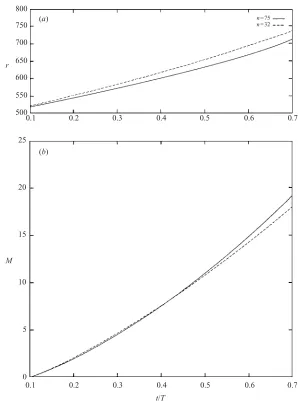
Figure 9.Development of the maximum value of|_{ωθ w}|for disturbance wavepackets generated

by impulsive excitation centred about re= 500 for n= 75 and n= 32. (a) Radial trajectories of the amplitude maxima; (b) magnitudes of the maxima plotted on a logarithmic scale. For bothn= 75 and n= 32 the magnitudes have been normalized so that they are equal to unity for t= 0.1T. With such a normalization, the quantity displayed in (b) is defined to be M= log2|ωθ w|max where the maximum is taken over all radial locations for each time instant.

magnitude of the maximum grows by a comparatively large factorO(26_{). During the}

second of the stated time intervals the maximum disturbance amplitude grows by a still larger factor O(27_{) and moves out to r 665. Figure 9 displays the trajectory}

and amplification of the wavepacket maximum, both for n= 75 and n= 32. From

0.002

0.001

0

– 0.001 – 0.002

0 0.1 0.2 0.3 0.4 0.5 0.6 0.7 0.8 0.9 1.0 (a)

(b)

0 0.1 0.2 0.3 0.4 0.5 0.6 0.7 0.8 0.9 1.0 0.10

0.05

0

–0.05

–0.10

(c)

0 0.1 0.2 0.3 0.4 0.5 0.6 0.7 0.8 0.9 1.0 3.0

1.5

0

–1.5

–3.0

0 0.1 0.2 0.3 0.4 0.5 0.6 0.7 0.8 0.9 1.0 80

40

0

–40 –80

t/T

(d)

Figure 10. Time histories forω_{θ w} (solid lines), together with corresponding envelopes±|ω_{θ w}|

(broken lines), for a disturbance withn= 75 that is impulsively excited atre= 550. (a)r= 525; (b)r=re= 550; (c)r= 575; (d)r= 600.

disturbance wavepacket maxima for n= 75 and n= 32 are evident from the plots of the magnitudes of the maxima that are plotted in figure 9(b). It can be seen that for early times, at least, the amplification experienced by the disturbance wavepacket, when measured in terms of the maxima of theωθ w, is not greatly different forn= 75 and n= 32.

1.4

1.2

1.0

0.8

0.6

0.4

0.2

0

525 550 575 600 625 650

t T

r

Figure 11.Spatio-temporal development of|ω_{θ w}|for an impulsively excited disturbance with

n= 75. The impulsive disc surface motion used to excite the disturbance was centred atre= 550. (Contours drawn using a logarithmic scale, with levels separated by factors of two.)

impulsively excited at re= 550 (see Point 3 in figure 2b) instead of at re= 500. The excitation now lies well inside the absolutely unstable region according to the SH linear stability theory of Lingwood (1995) – in fact, the situation corresponds to figure 3(b). It can be seen that there is temporal growth at all selected radial positions. In particular, the disturbance grows atr=re= 550. It also grows at r= 525< re. At this inward position the surface motion associated with the ‘impulsive’ forcing was relatively small, but not completely negligible. Nevertheless, we do not believe that the continual temporal growth observed at r= 525 is simply the localized response to a locally prescribed wall motion of small but finite extent. Temporal growth was not sustained at r= 525 for the previous case with re= 500 (see figure 5), yet the distance from the centre of the excitation is the same, albeit in the opposite radial direction, and consequently the small wall motion associated with the forcing would have been very similar. These differences in the disturbance behaviour at r= 525, between two simulations conducted with different forcing locations, show that there can be upstream information transmission in the radial direction. Stronger evidence for the existence of substantial radially inward propagation effects can be obtained by examining the overall development of the disturbance wavepacket forn= 75 and re= 550, using spatio-temporal contour plots, as before. From the contours displayed in figure 11 it is evident that, over the time interval considered, the trailing edge of the disturbance propagates along the inward radial direction, rather than radially outward as was the case when the excitation was applied at re= 500. However, it may also be observed that the temporal growth experienced by the disturbance at any given radial position remains rather weak in comparison with the convective growth revealed by tracing the wavepacket amplitude maximum.

1.4

1.2

1.0

0.8

0.6

0.4

0.2

0

525 550 575 600 625 650

t T

r

Figure 12. Spatio-temporal development of |ω_{θ w}| an impulsively excited disturbance in a

spatially homogeneous flow. The azimuthal mode number isn= 75 and the Reynolds number isR= 550. The arbitrary origin for the radial coordinate has been chosen so that the impulsive disc surface motion was centred atre= 550. (Contours drawn using a logarithmic scale, with levels separated by factor of two.)

more pronounced in the SH case. This is as might be expected. For the SI simulation, the radially inward direction corresponds to decreasing Reynolds numbers and hence decreasing instability for the disturbance. When the SH approximation is applied, all radial locations become equivalent because they are all associated with the same Reynolds number. Consequently, the disturbance is not subject to any stabilization as it propagates radially inwards. The effects of the mean-flow SI on the evolution of the wavepacket amplitude maximum are also as might have been anticipated. In the real SI flow the radially outward propagation exhibited by the amplitude maximum is associated with an increasing local Reynolds number, and hence with greater instability. Thus the temporal growth of the wavepacket amplitude maximum is enhanced, as may be confirmed upon making reference, once more, to the detailed differences between the contours plotted in figure 11 and figure 12.

Further comparisons between the data obtained from the SI and SH simulations reveals the existence of more subtle effects attributable to the mean-flow SI. Figure 13 contains a plot that illustrates the temporal evolution of the disturbance for the SH case withR= 550. The figure also includes a replot of the evolution obtained at the corresponding radial position re= 550 in the real SI boundary layer. It can be seen that the two plotted curves are quite close together for the early part of the time interval. However, over a longer time period, there is weaker accumulated growth in the SI case, together with a phase shift that is indicative of disparate temporal frequencies. Differences in the growth rates and the frequencies can be identified, in a more precise manner, by considering the complex-valued quantity defined by

˜ β= i

A ∂A

∂t,

0.3

0.2

0.1

0

–0.1

–0.2

–0.3

0 0.2 0.4 0.6 0.8 1.0 1.2 1.4

t/T

Figure 13.Comparison of the variation of ω_{θ w} for a disturbance with n= 75 evolving in

spatially homogeneous and inhomogeneous flows. The temporal development is shown for the radiusr=re where the impulsive excitation was centred. Solid line: inhomogeneous flow with

re= 550; dashed line: homogeneous flow withR= 550.

space or time, its real and imaginary parts may be interpreted as being, respectively, the local temporal frequency and the local temporal growth rate of the disturbance. This interpretation presumes that there is only a single mode of disturbance with a significant level of excitation at any specific radial location and time. The identification of the real and imaginary parts of ˜βas the unique local temporal frequency and growth rate would not be appropriate if there were a superposition of a number of discrete modes of disturbance, each with a different characteristic frequency.

–16

–17

–18

–19

–20

0.2 0.4 0.6 0.8 1.0 1.2 1.4

F

requenc

y

(i) (ii) (iii) (iv)

t/T

0.2 0.4 0.6 0.8 1.0 1.2 1.4

t/T

0.6

0.5

0.4

0.3

0.2

0.1

0

Gro

w

th rate

Figure 14. Local temporal frequencies ˜_βrRand temporal growth rates ˜_βiRfor a disturbance

withn= 75 in a spatially homogeneous flow forR= 550. The temporal development is plotted for four different radial positions: (i)r=re, (ii)r=re−25, (iii)r=re+ 25, (iv)r=re+ 50.

than for the frequencies. Thus for the SH flow, as expected from Lingwood’s (1995) analysis, a response of the form (3) is generated.

–16

–17

–18

–19

–20

0.2 0.4 0.6 0.8 1.0 1.2 1.4

F

requenc

y

(i) (ii) (iii) (iv)

t/T

0.2 0.4 0.6 0.8 1.0 1.2 1.4

t/T

0.6

0.5

0.4

0.3

0.2

0.1

0

Gro

w

th rate

Figure 15.Local temporal frequencies ˜β_rRand temporal growth rates ˜β_iRfor a disturbance

with n= 75 developing in a spatially inhomogeneous flow. The impulsive excitation was centred at re= 550. The temporal development is plotted for four different radial positions: (i)r=re= 550; (ii)r= 525; (iii)r= 575; (iv) r= 600.

difficult to carry out. Convergence problems were encountered with the iteration scheme used to solve the discretized governing equations, owing to the very large range of disturbance magnitudes that developed within the computational domain. In the absence of any nonlinearity, the maximum amplitude of the disturbance wavepacket was free to exhibit unhindered exponential growth. (For t/T ∼ 1.4 the maximum disturbance wavepacket amplitude was more than O(1020_{) times larger}

than the amplitude found at r=re. The incommensurability between the temporal growth at a fixed radial position and the growth obtained by following the trajectory of the wavepacket amplitude maximum was discussed above.)

These simulation results suggest that the global behaviour may well be convective. But numerical problems prevented us from continuing the simulations for a sufficiently long time to provide more definite evidence. To overcome these numerical problems we carried out another series of simulations for which re= 530 and n= 67. These parameters still lie well within the region of absolute instability – see Point 4 in figure 2(b) – but the absolute instability is less powerful than for the previous simulation. Figure 16 plots the variations in the temporal growth rates and frequencies corresponding to these new parameters for both SI and SH simulations. In this case the closer proximity to the boundary of the absolutely unstable region permits a more definite identification of the changeover from temporal growth to temporal decay. The locally defined growth rates and frequencies determined from the SI simulation are plotted for equally spaced radial positions, as before. For the SH simulation, the values for the temporal growth rate and frequency are only displayed for r=re, using the same axes as for the SI results. (The SH frequency agrees exactly with the absolute-instability frequency given by Lingwood (1995) for the same combination of parameters.) It is now clear that in the SI flow the growth rates eventually become negative for all monitored radial locations. Thus the disturbance shows a long-term decay after an initial period of growth. This is particularly marked for r=re where little growth occurs at all; for the more outboard radial locations there is much stronger transient growth before any decay sets in.

The results displayed in figure 16 strongly suggest that the long-term global behaviour is consistent with convective instability, i.e. the global behaviour is similar to that found in spatially inhomogeneous systems that are everywhere at most convectively unstable. The convective nature of the long-term behaviour is even more clearly apparent in the contrasting ray diagrams presented in figures 17(a,b). The SH simulation gives a pattern typical of absolute instability. For the SI simulation, on the other hand, the rays which initially propagate upstream, turn back on themselves in the manner suggested by figure 4(b). Although there is always room for doubt in any numerical simulation or physical experiment, the results displayed in figures 16 and 17 unmistakably indicate that the long-term global behaviour is not consistent with a linear amplified global mode of the form (3), i.e.

A∼e−iωGt_,

but is, instead, consistent with convective instability. This conclusion cannot be dismissed as being due to a minor adjustment in the boundary of the absolute-unstable region caused by SI. Numerical simulations conducted for both the SI and SH flows for different azimuthal mode numbers, and also for an impulsive excitation applied at much higher Reynolds numbers, provided firm evidence that the convective-like long-term behaviour is, in fact, typical.

0.2 0.4 0.6 0.8 1.0 1.2 1.4

F

requenc

y

(i) (ii) (iii) (iv)

t/T

0.2 0.4 0.6 0.8 1.0 1.2 1.4

t/T

Gro

w

th rate

(v) –14

–15

–16

–17

–18

0.5

0.4

0.3

0.2

0.1

0

–0.1

Figure 16.Local temporal frequencies ˜β_rRand temporal growth rates ˜β_iRfor a disturbance

withn= 67. For the curves labelled (i)–(iv) the impulsive excitation was centred at re= 530 and the flow is spatially inhomogenous. The temporal development is plotted for the radial positions: (i)r=re= 530; (ii) r= 505; (iii)r= 555; (iv)r= 580. The curves labelled (v) show the development at the point of impulsive excitation of a similar disturbance in a spatially homogeneous flow with R= 530. The constant frequency obtained from the simulation for the homogeneous flow is in exact agreement with the frequency of the absolute instability predicted by Lingwood (1995).

1.6

1.4

1.2

1.0

0.8

0.6

0.4

0.2

0

525 550 575 600 625 650

1.6

1.4

1.2

1.0

0.8

0.6

0.4

0.2

0

525 550 575 600 625 650

t T

t T

r

(a)

(b)

Figure 17. Spatio-temporal development of|ω_{θ w}|for an impulsively excited disturbance with

n= 67. The impulsive disc surface motion used to excite the disturbance was centred atre= 530. (a) Spatially inhomogeneous flow; (b) spatially homogeneous flow with R= 530. (Contours drawn using a logarithmic scale with levels separated by a factor of two.)

–14

–15

–16

–17

–18

0.2 0.4 0.6 0.8 1.0 1.2

F

requenc

y

t/T

1.2

1.1

1

0.9

0.6

0.2 0.4 0.6 0.8 1.0 1.2

Gro

w

th rate

t/T

0.8

0.7

(i) (ii) (iii) (iv) (v)

Figure 18.Local temporal frequencies ¯_βrRand temporal growth rates ¯_βiRfor a disturbance

2.4

2.0

1.6

1.2

0.8

0.4

0

300 325 350 375 400 425 450 475 500 525 550

t T

r

r_a

Figure 19. Spatio-temporal development of|ω_{θ w}|for an impulsively excited disturbance with

n= 67 andre= 311. ×, + denote experimental data points for the leading and trailing edges of the wavepacket taken from figure 15(b) of Lingwood (1996). (Contours drawn using a logarithmic scale with levels separated by a factor of two.)

In this case the disturbance was excited at a location even further into the region of absolute instability, at a radius that corresponds to approximately one and a half times the critical Reynolds number for the onset of absolute instability in the SH flow. This is very far beyond any radius at which the rotating-disc boundary layer has been found to remain laminar in physical experiments.

Comparison with Lingwood’s experimental data

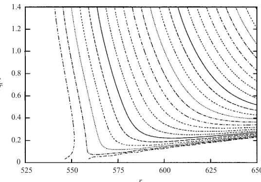
It is not possible to carry out a simulation that exactly mimics the experiment described in Lingwood (1996). Both the numerical and physical experiments generate the initial disturbances with excitations that roughly approximate a point impulse. Thus a wide range of frequencies and azimuthal wavenumbers are generated in each case. Lingwood excited the disturbances by a pressure pulse generated by a small transient jet that was triggered once per revolution of the disc. The precise spectral content of the initial experimental disturbances is not known, but it is likely to differ considerably from that of the numerically generated disturbances. Thus we cannot sensibly compare experimental and numerical wavepackets containing many different azimuthal wave-numbers because we have no way of knowing the relative amplitudes of the azimuthal modes in the experiment. All we can sensibly do is compare the numerically simulated development of an impulsively excited wavepacket containing a single azimuthal mode with that of the experimentally generated wavepacket. The logical choice for the single azimuthal mode is n= 67, as this is the first to become absolutely unstable.

the experiment. Now the impulse is located well inboard of the region of absolute instability – see Point 7 in figure 2(b). This situation corresponds to figures 3(a) and 4(a) and to Lingwood’s (1996) experimental investigation. Lingwood applied a pressure impulse through a hole in the rotating disc surface and then tracked the evolution of the leading and trailing edges of the resulting wavepackets. It can be seen that reasonably good agreement is found in figure 19 between the leading and trailing edges of the numerically simulated wavepacket and Lingwood’s experimental data. She argued that her experimental data for the trailing edge of the wavepackets could be fitted well by a curve that asymptoted to a constant radius ast → ∞. The constant radius selected corresponded, of course, to the critical value for absolute instability.

It is only fair to point out that the choice of threshold disturbance amplitude marking the leading and trailing edges of the numerically generated wavepacket in figure 19 is somewhat arbitrary. The choice of threshold amplitude makes little difference to the location of the leading edge, but the precise location of the trailing edge is quite sensitive to the threshold level chosen. In contrast, the slope of the trailing edge is insensitive both to the precise value ofn as long as it is fairly close to n= 67, and to the value of the threshold amplitude. Furthermore, only a single azimuthal mode is included in the numerical simulation, whereas the experimentally generated wavepacket contains a superposition of azimuthal modes. We have carried out similar numerical simulations for a range of azimuthal modes corresponding to values ofnbetween 30 and 75. The azimuthal mode withn= 67 is the first to become absolutely unstable. This is why it was chosen for figure 19. Forr > ra the value of

ncorresponding to the most unstable azimuthal mode rises. Asnrises up to n= 75, the slope of the wavepacket’s trailing edge tends to become steeper. The leading edge is insensitive to the value of n or r. It is plain from figure 19 that the n= 67 mode is initially damped for r > re. What probably happens with the experimental wavepacket is that at relatively low values ofr > re, it is initially dominated by the most convectively unstable modes (n∼30). But absolutely unstable modes dominate the wavepacket at later times asr →ra.

50

25

0

–25

–50

1.0 1.2 1.4 1.6 1.8 2.0 2.2 2.4

t/T

Figure 20.Variation ofω_{θ w}for a disturbance withn= 67 excited by an impulse centred at

re= 311. The temporal development is shown forr= 551.

from its source, there is a period of rapid temporal growth which is followed by equally strong decay.

–14.5

–15.0

–15.5

–16.0

–16.5

–17.0

–17.5

1.0 1.2 1.4 1.6 1.8 2.0 2.2 2.4

t/T

Figure 21.Variation of local temporal frequency ˜β_rR for a disturbance developing in the

spatially inhomogeneous flow withn= 67 excited by an impulse centred atre= 311. The solid line plots the temporal development forr= 551. The dashed line corresponds to the asymptotic frequency for the corresponding spatially homogeneous flow withR= 551.

Discussion

The outcome of our investigation of the global behaviour of the rotating-disc flow has certainly surprised us. To some extent it runs counter to conventional wisdom. Accordingly, we would expect our numerical methodology to be questioned and will now discuss some of the possible numerical pitfalls. It is well known that the inflow and outflow boundary conditions can lead to spurious effects, even when carefully implemented. For example, Buell & Huerre (1988) (cited in Cossu & Loiseleux 1998) showed that spurious, destabilizing, pressure-feedback loops can be generated by the influence of the numerical outflow boundary conditions on an upstream boundary, causing flows that are everywhere convectively unstable to exhibit spurious self-sustained oscillations in the numerical simulations. Kaiktsis, Karniadakis & Orszag (1996) also warn of the dangers of obtaining spurious results due to problems with the outflow boundary conditions when using numerical simulations to study global temporal modes. In their simulations of flow over a backward-facing step, they found that unless the computational domain was sufficiently long, the results were seriously affected when the disturbance was merely set equal to zero at the outflow boundary.

again (see §2) that, in our experience also, spurious temporal growth resulted when computational domains were so short that unwanted feedback occurred from the outflow boundary.

A different numerical problem has been recently revealed by Cossu & Loiseleux (1998). They have investigated the numerical dispersion relations obtained for the linear Ginzburg–Landau equation (see §1) using the Euler explicit and implicit, and Crank–Nicholson schemes. For example, in the case of the last of these three schemes, they found that in cases where an absolute instability should exist, there is a range of spatial step sizes for which it is impossible to obtain an absolute instability numerically, irrespective of the time step. This problem only existed for relatively small values ofµin (4). Nevertheless, it provides a valuable warning that numerically stable schemes may still exhibit spurious convectively unstable behaviour, or for that matter erroneous absolutely unstable behaviour. For our simulations, we used schemes with better stability characteristics than Crank–Nicholson (see I). But, probably, the best evidence that we were not unwittingly suffering from the problems analysed by Cossu & Loiseleux is the fact that our numerical simulations of the (artificial) spatially homogeneous flow always correctly identified the type of instability (i.e. whether absolute or convective), appropriate to the choice of flow parameters, in accordance with Lingwood’s (1995) stability theory. One final point may be worth makinga propos` the reliability of the computational results. This concerns our use in I of an inertial frame fixed with respect to the rotating disc for the formulation. Recently we have reformulated the governing equations and numerical schemes in terms of a fixed laboratory coordinate system. The results thus obtained were indistiguishable from those presented here.

The picture emerging from our simulations is summarized schematically in figures 4(a) and 4(b). The long-term global behaviour appears to be convective in the real spatially inhomogeneous flow. The absolute instability does not lead to sustained temporal growth. However, there is strong, localized, temporal growth, accompanied by upstream (inboard) propagation, over relatively short time scales. In this respect the behaviour is not unlike localized algebraic growth. This localized growth would ensure that the already existing, strongly growing, convective disturbances grow very strongly in the vicinity of the absolute instability. This localized growth is likely to be more than sufficient to bring in the nonlinear effects that govern the final stages of transition. The associated short-term upstream propagation would also ensure that the transition point was well-defined and not sensitive to background noise. Thus the picture revealed by the simulations and depicted in figures 4(a) and 4(b) is fully consistent with Lingwood’s (1996) experiments.

Compliant annulus

Figure 22.Schematic sketch showing a compliant annulus set into the disc surface.

4. Numerical simulations for compliant rotating discs

The formulation and numerical methods described in I allowed us to make part of the disc’s surface compliant. In fact, results were presented in I showing the evolution of disturbances generated by periodic wall forcing in the boundary layer over a disc with a compliant annulus, as shown schematically in figure 22. It was shown that the Type I disturbances were subject to significant stabilization. The stabilizing effect on the Type II disturbances was found to be much weaker, with negligible modification to radial growth rates. In both cases the surface stiffness parameters that characterize the spring-backed plate model used for the compliant part of the disc were chosen so as to avoid the onset of flow-induced surface instabilities. It was noted that our numerical simulation results in I were in broad agreement with the linear stability results obtained by Cooper & Carpenter (1997a) for a compliant surface formed from a single visco-elastic layer.

We will now present the results obtained from a numerical simulation of the development of a disturbance generated by an impulsive excitation of the real spatially inhomogeneous flow when part of the rotating-disc surface incorporates a compliant annulus. As in one of the numerical simulations described before, the azimuthal wavenumber of the disturbance wasn= 75 and the prescribed impulse centred around re= 550. The surface was compliant over an annular region ranging from r= 600 to 650. (The inner radial boundary of the compliant annulus thus lies well beyond the experimentally observed transition point. It also lies well within the absolutely unstable region determined by Lingwood’s linear stability analysis. Similar, but less clear, effects were obtained when the inner boundary of the compliant annulus was located at a smaller radius.) The non-dimensional surface compliance parameters were selected in accordance with the optimization scheme described by Carpenter & Morris (1990). The flow-induced surface modes were expected to be, to a first approximation, marginally stable at the outermost radius of the compliant insert. The non-dimensional critical wavenumber, ¯αd, for the divergence mode, in terms of which the optimized compliant surface parameters could all be expressed, was chosen to have the value 0.2.

0.10

0.05

0

–0.05

–0.10

0 0.1 0.2 0.3 0.4 0.5 0.6 0.7 0.8 0.9 1.0

t/T

(a)

0 0.1 0.2 0.3 0.4 0.5 0.6 0.7 0.8 0.9 1.0

t/T

(b) 3.0

1.5

0

–1.5

–3.0

0 0.1 0.2 0.3 0.4 0.5 0.6 0.7 0.8 0.9 1.0 (c)

20

10

0

–10 –20

0 0.1 0.2 0.3 0.4 0.5 0.6 0.7 0.8 0.9 1.0 (d)

200

100

0

–100

–200

t/T

t/T

Figure 23.Time histories of_{ωθ w}(solid lines) for a disturbance with azimuthal mode number

n= 75 that is impulsively excited atre= 550. The disc surface is compliant for 6006r6650. Amplitude envelopes±|ωθ w|are also shown (broken lines), both for the simulation with the compliant insert and for a corresponding simulation where the disc surface was entirely rigid. (a) r=re= 550; (b)r= 575; (c)r= 600; (d)r= 625. The surface compliance parameters are such that, notionally, there is marginal stability with respect to divergence and travelling wave flutter modes at the outermost radius of the compliant annulus. The critical wavenumber for the compliant surfaces is ¯αd= 0.2.