Developing and testing an APP model for Air Spiralo

(1)

Supervisors:

Dr. Matthieu van der Heijden, University of Twente

Dr. Leo van der Wegen, University of Twente

Dave van Diepen, Air Spiralo

®

Developing and

testing an APP model

for Air Spiralo

®

A master thesis by:

(2)

i

Preface

As industry 4.0 starts to have its effect on the performance of production, it is important for a company to be able to analyse any changes in required capacities and inventory quickly. By increasing the performance of production, the manufacturing lead time will decrease and efficiency will go up. It also happens often that knowledge is not captured in a decision making model. As a result, this knowledge is lost when the person leaves the company. So, to follow the effects of improving efficiency in production and to capture every bit of this knowledge, it is sensible to create a decision making model that is able to make decisions on a tactical planning level and takes the objectives of the optimal solution into consideration. For this, the aggregate production planning (APP) model has proven to be very useful. This study, therefore, aims to create such an APP model and allow the company to capture every bit of knowledge from different departments into one place.

Upon completion of this master thesis, I am finishing the master program “Production and logistics Management” from the Industrial Engineering and Management study at University of Twente, Enschede. During this master program, I have been able to grow a lot as a person. I have become a person who is capable of leading a project as well as analysing difficult engineering problems. And also, I have grown confident in applying the theoretical knowledge from my study into day to day situations at a company. I am therefore grateful to have done my master program at the University of Twente and have the help of some great and inspiring people.

Still, despite my own skills and experiences, I could not have finished this master thesis without the help of my supervisors at the University of Twente. I would, therefore, like to thank Matthieu van der Heijden and Leo van der Wegen for having the patience while supervising me during this research and giving a constant flow of positive feedback. And, furthermore, I would like to thank Dave van Diepen, who was my supervisor at Air Spiralo®, for helping me get the correct information and sharing his knowledge every day.

(3)

ii

Summary

This study focuses on the company Air Spiralo®, which is located in The Netherlands, Poland and Finland. The company is specialised in producing ventilation ducts and fittings for housing, utility and industry. The main production facility is located in Poland and operates according to the Make-to-Order strategy. As a result, the managers at the facility in The Netherlands have to make sure the production facility in Poland is manufacturing the right products as well as the correct quantities. Unfortunately, the managers at Air Spiralo® are not able to make a good tactical production plan since they currently only use the first three months of each demand forecast to calculate the production plan. As a result, the company has to cope often with insufficient labour capacity or high inventory levels as they are trying to follow the demand behaviour over the year.

Based on this problem description, two research goals were drafted. First, this study mainly aims to find a production planning model, which is able to plan production on a tactical planning level and also include preferences and requirements mentioned by the managers at Air Spiralo®. Second, this study aims to use the production planning model to find the optimal production plan for the year 2016 and give some recommendations about the use of workers and/or machines at the manufacturing facility in Poland.

To find the requirements for the production planning model, interviews were conducted with managers in The Netherlands and Poland. Based on these requirements, production planning models were searched for in literature that included some of the requirements. Then, the results from the literature review were used to set up the production planning model for Air Spiralo®. This production planning model was than validated with historical data, such as sales history, from 2015 and the manufacturing cost prices of individual products. Finally, the production planning model was used to find the optimal production plan for the year 2016. Here, the budgeted amount of worker FTE as well as the expected sickness and holiday leave for the year 2016 was used.

The main results of the first research goal are:

- An Aggregate Production Planning (APP) model was set up, which will search for the lowest possible total cost to meet a given demand forecast for a rolling horizon of 12 months.

- The total cost includes production hours of workers, both through regular time as well as overtime, and machinery. Furthermore, the total cost is also a summation of the holding costs for each period; which is dependent on the number of stored pallets. - This holding cost is a result of storing items in two different storage locations.

Because the cost rate for storing a pallet is different for these two locations, a piecewise linear holding cost function was included in the APP model.

(4)

iii

The main results of the second and final research goal are:

- The optimal manufacturing strategy for Air Spiralo® is to follow the level strategy in which inventory is built up in periods of low demand to meet demand in periods where regular production capacity is insufficient.

- A brief sensitivity analysis showed us that the current holding cost of the regular warehouse is only allowed to increase at most 60% before the decisions of the APP model are changed significantly.

- We also found during the sensitivity analysis that the parameter value for overtime production is only allowed to decrease with 40% before the decisions of the APP model are changed significantly.

- It is profitable to lower the number of FTE in production from the current budgeted 80 to about 75. Total yearly cost will increase with about €7,000 because the APP model will have to plan production through overtime, but this is far less than the cost of having to pay five workers in production.

- It is interesting for Air Spiralo® to try and improve the productivity of workers in production. By improving productivity with only 2%, the objective value of the APP model decreases with €3,647. Moreover, such an improvement in productivity also means Air Spiralo® will also mean they will roughly need 2 production workers less. This, in the end, translates to a yearly cost saving of €23,647.

From the output of the APP model, we found quite a different production plan as is currently followed at Air Spiralo®. The APP model showed that it is best for Air Spiralo® to keep production level and build up capacity stock in periods of low demand in order to meet high demand in other periods. At the moment, the available inventory capacity at the manufacturing facility in Poland is not used for any capacity stock such as this. Therefore, the managers at Air Spiralo® have to try and implement such a manufacturing strategy at their manufacturing facility in Poland. Furthermore, the managers have to try and get familiar with the way the APP model uses. To help realise this, we have written a manual in which the purpose and usability of the APP model is briefly described. But also, this manual explains who should be made responsible for making sure the data is correct and accurate every time the APP model is run.

(5)

iv

Chapter 1 Introduction

1.1 Company description

1.1.1 History

The company Air Spiralo® is specialised in producing ventilation ducts and fittings for housing, utility and industry. The company was founded in 1840. Back then, the core business was producing copper. After 1940, the company started producing central heating equipment and ventilation ducts next to their core business. Then, in 1992, the family De Haan took over Kennemer Schagen B.V., which is the part of Air Spiralo® that is located in The Netherlands, and changed the company's name to Kennemer Spiralo®. In 1993, the company opened their manufacturing facility Kentel in Poland at which their main production activities are currently situated. Since 2005, the whole company introduced the international company name Air Spiralo® and the core business was changed to the production of ventilation ducts and fittings. Finally, in the year 2008, a family company in Finland, which is highly specialised in manufacturing pressed fittings, was included in the Air Spiralo® group to manufacture a part of the product mix of Air Spiralo®.

1.1.2 Geographic orientation of Air Spiralo®

The company Air Spiralo® is a supplier for a broad range of customers, regarding both geographic dispersion as well as types. Their customers are located in, for example, The Netherlands, Belgium, Norway or England. And regarding customer types, Air Spiralo® supplies both wholesalers, such as Technische Unie in The Netherlands, as well as ventilation specialists. These different kinds of customers all supply a different kind of market, which results in a different kind of demand behaviour.

Furthermore, the company Air Spiralo® is divided up into several semi-decoupled companies. The company Kennemer Spiralo® is located in the Netherlands and is responsible for supplying and contacting the customers; therefore, the warehouse is also situated here. And, because this facility is mainly responsible for supplying the end-customers, the customer order decoupling point (CODP) is placed close to the end-product. And so, in order to be able to deliver the customer from on-hand inventory, this facility operates according to the make-to-stock (MTS) strategy.

(9)

2

finished at Kentel. At the moment, these semi-finished products are first transported to the Netherlands to make sure that the company is able to send full trucks to Kentel. The idea is to transport these semi-finished products from Air Spiralo® Oy to Kentel directly in the future. Some parts of the finished-products are difficult to manufacture and require some more specialisation. These parts are, for example, fire dampers or motorised air regulators. Because the company does not want to be involved in manufacturing these products themselves, they purchase these products at other suppliers. All those parts will be sent to Kennemer Spiralo® first, where they distribute the necessary parts to Kentel. There, they assemble it to the finished products.

[image:9.595.116.430.260.568.2]

In the end, the total supply chain of Air Spiralo® could be shown graphically as follows. The dotted lines represent flow of information and the full lines represent physical flow of items.

Figure 1 - Supply chain of Air Spiralo®

From this figure, it becomes clear that everything is managed from the location Kennemer Spiralo®. The production orders are sent from this location to the manufacturing facilities and also the customers are being supplied from this location.

1.1.3 Examples of projects and innovation

(10)

3

1.2 Motivation of the research

1.2.1 Problem description

By making sure that the customer receives the products as much as possible on the requested date, the company is able to distinguish itself from competitors. But, being able to deliver all demand as much on the requested date asks for a flexible manufacturing process or, otherwise, high inventory levels. Unfortunately, it takes quite some time to perform a set-up on a machine for producing a particular product. Therefore, the manufacturing facilities use batches in their production process to be able to manufacture more efficiently. This creates a mismatch between the goal of the company and reality. Adding to this problem, the number of available workers at Kentel cannot be changed easily; thus making production not very flexible. The reason for this is that it is difficult to find the rightly skilled workers and training them for the required operations takes quite some time. As a result, the company is also not able to increase the worker capacity in order to meet high demand.

Furthermore, as we briefly explained in Section 1.1.2, the manufacturing facilities operate according to the MTO strategy. As a result, these facilities can only react to the renewed production forecast that is provided by Kennemer Spiralo®. It is, therefore, the responsibility of Kennemer Spiralo® to make sure that the facilities in Poland and Finland keep producing the right amount of products necessary to fill the inventory levels. For example, if demand is significantly higher than expected, the re-order level is reached earlier. As a result, the inventory manager will send a renewed production forecast to the manufacturing facility earlier than the monthly update, as some sort of urgency order. And because the manufacturing facilities already have to sometimes cope with insufficient capacity, these urgency orders put a lot of pressure on this workers capacity at the manufacturing facilities. Furthermore, the production forecast, and therefore the production planning, is currently done on a three-month basis. Only these three months can be forecasted with enough certainty by the company with the resources they currently have. For all the other months of the year, no prediction is done about expected production orders and related capacities. As a result, it is very difficult for the company to analyse the tactical strategies regarding their inventory and production.

And finally, the company is expecting sales to grow in the near future. A significant grow in sales would ask for some big changes, such as expansion of the warehouse or the manufacturing facility. But, because the managers do not analyse production forecasts on a tactical level, the managers have little information about the necessary machine or worker capacities.

1.2.2 Objective of the research

(11)

4

It will be interesting to see if the APP model finds it optimal to produce around the same number of items each month or that it is best to wait for an increase in demand.

Furthermore, the APP model will include multiple time periods and can, therefore, try to prevent major under- or overproduction by planning production over a longer period. As a result, instead of creating new schedules every time demand is significantly different from the forecast, only a small adjustment will have to be applied to this monthly schedule.

And finally, a major advantage of the APP model is that it can be made according to the wishes and requirements of the managers at Air Spiralo®. This allows us to build the model such that it reflects the situation at Air Spiralo® as much as possible. Only when it reflects the situation well, the output of the APP model will be most reliable.

1.2.3 Research questions

One of the important aspects in this research is that the APP model will have to be built according to the wishes and requirements of the managers at Air Spiralo®. For this, we will need to conduct interviews in order to discuss these wishes and requirements. Furthermore, data will have to be analysed to make sure that the correct information is used in the APP model. Relevant data could be the production costs per unit or number of available employees for production. And finally, the APP model will also have to be verified and validated to assure that the model represents the situation at Air Spiralo® as good as possible.

All these different tasks are based on a core research question. In this thesis, the following research question, which is based on the problem description, is formulated,

"How could Air Spiralo® plan production and inventory over a longer planning horizon and decrease production nervousness in production as a result?"

In order to find the answer to this research question, a few sub-questions will have to be answered. We will discuss the following sub-questions in this thesis, which are automatically converted into chapters.

Chapter 2: Description of current production process and model preferences a. How are products manufactured at Kentel?

b. What information is used to calculate the inventory levels? c. What information is included in the sales forecast?

d. How is the sales forecast translated into a purchase/production forecast? e. What problems are present in the current way of working?

i. Is seasonal demand an important aspect? ii. Is overtime production often necessary? iii. Is worker capacity always sufficient?

(12)

5 Chapter 3: Literature review

a. What is the purpose of an APP model according to literature?

b.

Which kinds of APP or other production planning models have been developed in literature that incorporates the preferences of Air Spiralo®?

Chapter 4: Description of APP model for Air Spiralo®

a. How can we create an APP model for Air Spiralo® with the results from the literature review?

b. What are the parameters and decision variables of the model? i. What is the most suitable aggregation level?

ii. What are the values for the different model parameters? Chapter 5: Validating the APP model of Air Spiralo®

a. Is the APP model able to find the correct production cost from a given demand forecast?

b. Are the wishes and requirements, as given by the managers, modelled correctly in the APP model?

c. How sensitive is the APP model to the characteristics of the product group types?

Chapter 6: What does the APP model give as an optimal production plan?

a. What does the optimal production plan from the APP model look like for the year 2016?

b. What are the required capacities, regarding labour and machines, according to the APP model?

c. What is the best strategy for Air Spiralo to follow, i.e. chase, level or hybrid strategy?

d. On which aspects can Air Spiralo® improve with regard to production? Chapter 7: Implementation of APP model at Air Spiralo®

a. How often should the APP model be evaluated? b. What are the benefits of using the APP model?

c. Who should be made responsible for updating parts of the APP model? 1.2.4 Research approach

(13)

6

After we understand the different process steps within the company, we will perform a literature review regarding APP and other production planning models. First, we will briefly explain the concepts of an APP model. After that, based on the wishes and requirements, we will perform a literature review to find relevant articles regarding APP and other production planning models.

Based on the results from the literature review, we will give a description of the theoretical APP model for Air Spiralo®. We will describe the design of the APP model and the information that is included in every part of the model. And along with this description, we will also explain how we have defined the different parameter values in the APP model. For example, one of the important aspects of the APP model is the choice of aggregation level. These choices will be based on an analysis of data at Air Spiralo®.

After that, we will perform some validation tests on the APP model such that we can assure the managers at Air Spiralo® the model reflects the situation at Kentel correctly. In one of these tests, we will analyse whether the same production costs are found from the output of the APP model as from the cost prices at Kentel. But, we will also investigate how sensitive the model is to any changes in parameter values of product group mixes.

Finally, after we have established that the model works correctly, we will let the APP model search for the optimal solution for the demand forecast of 2016. Furthermore, we will also investigate how much overproduction would be necessary according to the APP model with respect to the current situation. And finally, we will briefly give an indication of how the business processes are changed as a result of the APP model, along with a brief description of the implementation method.

1.3 Scope of research

For a model such as the APP model, it is important that the input is as good as possible. For every decision making model, the output can only be as good as the input. Besides the challenges in production planning, we have also seen that the company is struggling with demand forecasting. But, as we have mentioned in Section 1.2.1, the company is also not able to find the necessary capacities and production quantities from any given demand forecast. So, while it could be interesting to improve the forecasting methods, we will choose to focus on building an APP model such that the company can analyse the effects on the business from any demand forecast input.

(14)

7

1.4 Outline of report

(15)

8

Chapter 2 Description of current situation

In Section 2.1, we will describe how the manufacturing facility Kentel is designed and how products, in a broad sense, are manufactured. Then, in Section 2.2, we will describe how Air Spiralo®, currently, manages its production planning process. By describing this process, we will understand what kind of information is available to implement in the APP model and, more importantly, what kind of information is missing. And furthermore, by describing this process step by step, we will probably come across some problems that are present at Air Spiralo®. We will discuss these problems in Section 2.3.And finally, in Section 2.4, we will end this chapter by describing the wishes and requirements, given by the managers at Air Spiralo®, regarding the APP model.

2.1 Manufacturing process at Kentel

As we have mentioned in the scope of this research, the APP model will only focus on the manufacturing facility Kentel. To understand how products are manufactured, we will briefly describe the manufacturing process in this section.

At the moment, the facility is mainly designed as a shop floor. This means that a specific manufacturing process, for instance the cutting process, is set up as a work centre in which multiple machines are available that can perform the process. After a product has gone through the process it is moved to the next cluster. If this cluster is already occupied, the product has to wait as work in progress (WIP).

The first stage is to cut 2D plates from a coil or sheet. This cutting can be done with a cutting knife or with a laser/plasma cutter. After cutting, these 2D plates are bent or rolled to create the 3D shape. Then, after the products are bent in the preferred shape, the 3D parts are welded together at the welding station. Here, the products are either point or line welded. Whether it can be welded on a machine mainly depends on the product type and the diameter. Large diameters are difficult to handle on machines because of their size. Therefore, those products are often manufactured by hand. One important aspect is that the number of required operations depends a lot on the product characteristics. For example, a silencer, from the CS product group, goes through the seaming process, while a duct coupling, from the SV product group, does not require this process. Furthermore, as mentioned in Section 1.1.2, some parts, such as motorised regulators, are purchased from external suppliers. If a product needs, for example, such a regulator, it is installed during one of the final stages.

After all the necessary processes have been performed, most of the products go through what is called the rolled over edge (ROE) process. This process has been introduced to create a Soft-Edge® onto the products. And with this Soft-Edge®, the products can also be fitted with the rubber seal, i.e. KEN-LOK® seal, to enhance the air tightness of the ventilation system. The addition of the Soft-Edge® has enhanced safety during installation dramatically. In the past, the products were simply sold with a sharp metal edge. As a result, the installer often cut himself on these sharp metal edges during instalment.

(16)

9

2.2 Production planning at Air Spiralo

®

2.2.1 Inventory management

Because manufacturing and inventory levels are closely related, we will briefly describe the inventory policy currently applied at Air Spiralo®. A more detailed description of the inventory calculations can be found in Appendix B. As we briefly explained in Chapter 1, the company Kennemer Spiralo® is responsible for supplying the end-customer and, therefore, operates according to the MTS strategy. To maintain this MTS strategy, the company makes use of

the (𝑠, 𝑆)-inventory policy. This policy is applied to both the semi-finished as well as the

finished products. The products with large diameters held as inventory consist of flat (semi-finished) sheets, which are later formed into an end-product.

The (𝑠, 𝑆)-inventory policy means that the manufacturing decisions are based on a re-order

level 𝑠 and an order-up-to-level 𝑆. Furthermore, because the main goal of the company is to maintain the highest possible delivery reliability towards the customer and lead time demand is uncertain, the inventory manager has set a service level target. At the moment, the company has chosen to use the „cycle service level‟ for their inventory model. The cycle service level states the probability of not stocking out in a replenishment cycle (Chopra & Meindl, 2007). Currently, a cycle service level of 94 percent is used to make sure they are able to deliver the customer from on-hand inventory.

To achieve this service level, the company makes use of a safety stock. This safety stock should account for the uncertainty in lead time demand. On top of this safety stock level, the re-order point 𝑠 is placed. This re-order point 𝑠 is placed such that the inventory level, on average, reaches the safety stock level upon delivery. So, this re-order point is equal to the safety stock level plus the average demand times the delivery time.

Then finally, the order-up-to-level 𝑆 is calculated. When inventory reaches re-order point 𝑠, the order-up-to-level 𝑆 determines how much should be ordered. For the situation at Air Spiralo®, this order-up-to-level 𝑆 is calculated such that an integer number of pallets or boxes are ordered. This is to ensure the optimal use of truck capacity. Furthermore, the managers have stated an optimal replenishment frequency per product class. In total, three different product classes have been defined through the ABC classification. At Air Spiralo®, this ABC classification is based on the cost price and the yearly sales of the product. For product belonging to class A, the products are ordered on full pallets. For the class B and C products, orders are placed in units of full boxes.

2.2.2 The sales forecast

Every month a sales forecast, given as an Excel spreadsheet, is released by the sales department. This sales forecast is mostly based on monthly invoices and is, therefore, expressed in amount of Euros per customer per country and per month. The customers per country are further divided up into classes. For instance, the wholesalers are separated from the ventilation specialists. Furthermore, the sales forecast only includes the forecast for the current month and the next two months. With the information that the company can gather, these three months can be forecasted with enough certainty; other months are only included in the forecast for the total year.

(17)

10

forecast is given. The rolling forecast is given by the sales department and shows how much the managers from the sales department think they can realise in the respective month or year. The financial budget, which is based on historical sales, states how much the company should be able to realise with full certainty for the respective month or year. The commercial budget is set as a target for the sales department to realise in the respective month or year. Finally, the mathematical forecast is calculated by multiplying the realised sales of that month by the number of workdays in that month and dividing it by the current workday number, thereby ending up with an expectation of the amount of realised sales for the current month. Finally, for the current month, the realised orders can be seen as well. The values for these realised orders, still given in Euros, are updated daily.

2.2.3 The production forecast

So, because the sales forecast is given in amount of Euros, the company does not know how much it has to produce of each individual end-product. To get this information, the sales forecast, described in the section above, is first translated into a sales forecast per country by summing up the forecasted sales for each customer in the respective country. This translated sales forecast, still expressed in Euros, is then forwarded to the inventory manager.

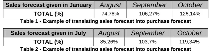
From this sales forecast, the inventory manager calculates a month-specific seasonal factor by comparing the sales forecast from the start of the year to the most recent sales forecast. A brief example can be found below.

[image:17.595.114.479.383.473.2]

Sales forecast given in January

August

September

October

TOTAL (%) 74,78% 106,27% 126,14%

Table 1 - Example of translating sales forecast into purchase forecast

Sales forecast given in July

August

September

October

TOTAL (%) 85,26% 103,7% 119,34%

Table 2 - Example of translating sales forecast into purchase forecast

In the first table, we can see how the sales forecasts for the months August up to October relate to a full year, i.e. a full year representing 1,200% (100% times 12 months). These values were estimated at the start of the year in January. The second table shows the sales forecast for the same three months at the start of July. Here, we can see, for example, that the sales forecast for August has increased with 10.48%. So, sales for that month has increased quite a bit but is still below average. If the inventory manager would, then, work with the average monthly sales as a sales forecast for August, he would overestimate the sales for August with 14.74%, i.e. the difference between 85.26% and 100%. So, to account for this change, the average historical sales for the individual end-product are multiplied with 85.26% for the month August. This means that the data from Table 1 is only used by the inventory manager to check how much demand has changed and whether this change is significantly different. Furthermore, these three months also show how much sales can differ between months. The month August is clearly a month in which sales is low and the month October is a month in which sales is high. Our APP model should be able to tackle such a difference by planning production quantities over a longer time horizon.

(18)

11

yearly sales forecast exists, the inventory manager will simply use the sales from recent 12 months as a sales forecast for that specific end-item in a full year.

With these forecasted sales quantities, the Excel spreadsheet checks whether the re-order point 𝑠 is reached at any moment in the upcoming three months. If the re-order level is reached for any product, a production order is placed for that particular month.

Then finally, the determined production orders are shown per end-product per month for the next 3 months as a production forecast. Because the operational production planning is mainly left to the production managers of Kentel, this production forecast is also called a purchase forecast. Unless something drastically changes in the sales forecast, for example a new customer arrives, this production (or purchase) forecast is only recalculated every 2 months. This means that the third month in the production forecast only functions as an indication. This three-month overview is sent to Kentel, from which they will assess whether their current workers capacity will be sufficient. If they think they will be able to manufacture the forecasted amount, they will accept the production orders. And, unless the inventory manager changes the production forecast, this capacity check is not done for a whole month. Our APP model will improve this situation by analysing more than three months. First, the forecast for these three months will be inserted. Then, for all the other months in the planning horizon, we will use the more roughly demand forecast such that we can still show the seasonal trend over the planning horizon. By planning production over a longer horizon, we allow the managers at Kentel to anticipate on changes a lot better in the future.

2.3 Analysis of current problems

Now that we understand the different steps in the production planning, we can analyse some problems which are present at Air Spiralo®. These problems are discussed in the following sections.

2.3.1 Overtime production analysis

As we already mentioned in the introduction, the company has to cope with quite some overtime during the production process at Kentel. It is, therefore, interesting for us to analyse the use of overtime in recent periods. This could show us how important it is for the APP model to analyse whether overtime is actually the cheapest option.

(19)

[image:19.595.94.501.66.278.2]

12

Figure 2 - Productivity at Kentel

We can also see, in the figure above, that overtime was necessary in every month. And the amount of overtime has been decreasing in the last couple of months. This decrease has been a result from the fact that the managers have noticed that overtime has been a dominant factor each month and have spent more attention to the causes of overtime. It will be interesting to see how much overtime the APP model will plan each month. At the moment, the managers have been trying to tackle overtime since they see it as something negative. But with the APP model output, we could see if overtime is really that negative. For example, it could be that it is actually cheaper to sometimes use overtime production instead of holding inventory for multiple periods. At the moment, the company is not able to analyse this.

One other remarkable point is that the amount of employees that have been reported as „sick‟ is quite high. From Figure 2, we can see that about 10% of total FTE has been reported as sick in each month. Trying to reduce these numbers could have a major impact on the use of overtime. Unfortunately, we are not able to influence such a problem in this research. But this analysis shows it is a problem that the company should think about resolving.

2.3.2 Workforce capacity analysis

(20)

[image:20.595.104.495.66.287.2]

13

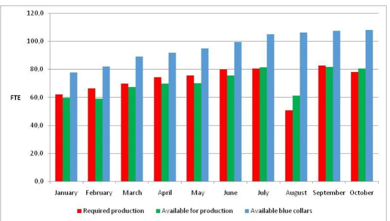
Figure 3 - Required production FTE against available workforce FTE

In this figure, we can see that for most months the amount of planned production has been demanding more than the available workforce FTE. Only in the months July and August enough worker-capacity was available. This could be a useful month to try and build up inventory for other periods. Furthermore, we can see that if we add, for example, the amount of FTE reported as „sick‟, from Figure 2, to the „available for production‟ here, the company would not have had any issues throughout these 10 months. This again shows that the amount of „sick‟ employees is a critical problem at Kentel.

We have also plotted the total available blue collar FTE, shown in blue. The available blue collar FTE is the same data as used in Figure 2, when comparing it to the used overtime per month. Comparing the „available blue collar‟ FTE to the „required production‟ FTE, we can see that the company, actually, has enough workers employed. But, as we could also see in Figure 2, quite a lot of FTE is used for other purposes. As a result, the company has to deal with an insufficient available capacity for production. In our research, because we build a production planning model on a tactical level, we will not be able to directly change the productivity at Kentel. But, by analysing available capacity of each month with the APP model, we can try to attune production to the available workforce capacity better and, thereby, lower the differences we see in Figure 3.

2.3.3 Inventory levels at Kentel

During the planning horizon, the APP model can choose to hold items on stock. At Kentel, inventory is not so much necessary to reach, for example, service levels. But, it can be used in periods where regular production time is insufficient and overtime hours are a lot more expensive or not allowed. So, it actually acts as some kind of extra source of supply in times where regular capacity is insufficient.

(21)

[image:21.595.76.527.67.235.2]

14

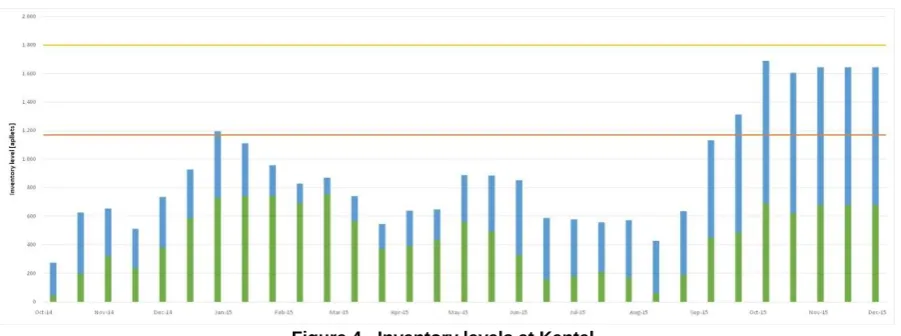
Figure 4 - Inventory levels at Kentel

In this figure, we have plotted two different boundaries for the inventory levels. In our APP model, these two boundary levels will be checked to see what holding cost rate should be applied. As long as the inventory levels stay below the orange line, the pallets still fit in the regular warehouse. The yellow line shows how much extra storage capacity is available at a different storage area at Kentel. For the pallets stored in this extra storage space, a different cost rate will be applied. Still, in total, the inventory levels may not exceed this yellow line because that is physically not possible. Furthermore, we have plotted the products from the RB product group separately as green bars. Because there is no space left in the warehouse of Kennemer Spiralo®, the managers have chosen to keep those items on stock at Kentel. On average, the inventory levels for the RB products is equal to 460 pallets, but in total 843 pallet places have been reserved for the storage of these products. Finally, the blue bars show us how much temporary inventory is used besides this RB inventory.

From this figure, we can see that the temporary inventory levels are quite high. At Kentel, products are, apart from the RB type, manufactured according to the MTO strategy. So, in theory, this temporary inventory should be zero in most cases. First, the big inventory increase in August 2015 is a result of the fact that required production is less than the available FTE. The cause of this can also be seen in Figure 3. There, the „available for production‟ has been bigger than the „required production‟ in the months July up to October. Because the company wants to keep producing items on a steady rate, i.e. not lay-off any workers, the company has been building up inventory in anticipation of future demand; even beyond the regular warehouse capacity. When demand increases again in the future, Kentel is able to deliver products from on-hand inventory and they will need less FTE for immediate production. This is something that our APP model will analyse as well. In the months where worker capacity is left over, the model will decide whether it is a good option to produce extra items which it will hold on stock. So, it will be interesting to see how the inventory levels from our model will look compared to this figure.

(22)

15

items waiting for shipment. Again, it will be interesting to see if the APP model finds those numbers to be optimal as well during the planning period.

2.3.4 Analysing seasonal demand

[image:22.595.73.525.245.387.2]

An APP model is extremely useful for situations where seasonal effects come into play during the planning horizon. If these seasonal effects are present, an APP model should be able to tackle it by planning production optimal over a longer period. To analyse the seasonal effects at Air Spiralo®, we have plotted accumulated monthly demand of all products between the year 2013 and 2015 in the figure below. In this figure, the green line shows demand in the year 2013, the orange line shows demand in the year 2014 and, finally, the red line shows demand in the year 2015. For the company‟s sake, we have left out the values on the vertical axis.

Figure 5 - Monthly demand for all products over 2013-2015

One thing that stands out immediately is the low demand around the month December. What happens is that the company is closed for two weeks around the turn of the year because of the Christmas holidays. Just before that period, we can see that demand increases in November. In that period, customers start to order more products to also fill their inventory levels as the calendar year closes.

Besides that, one other big seasonal effect we can derive from Figure 5, is the demand behaviour in the summer periods. Around the weeks of July, the construction holiday starts. In that period, construction comes to a hold and, therefore, demand for the products of Air Spiralo® decrease as a result. In previous years, the manufacturing facility Kentel was also closed in that period. The result of that can be clearly seen in the year 2013 and 2014 where demand decreases a lot around the month July. Furthermore, most of the workers at Kentel, as we saw in Figure 2, go on holiday as well. Therefore, not a lot of workers are available for production. But, as Figure 3 has shown us, the required production is still under the available capacity. As a result, these summer holidays could be a useful period in the APP model to plan extra production and build up inventories for other periods if that turns out to be the cheapest option.

(23)

16

model as it will have to try and tackle such a peak demand with the little worker capacity that it is given.

2.3.5 Analysing demand behaviour of end-products

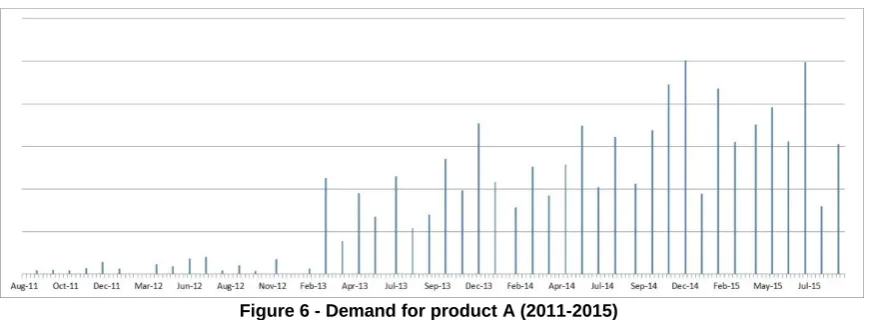
[image:23.595.83.518.257.417.2]

Besides the importance of seasonal effects during the planning horizon, it could also be beneficial to aggregate demand because of the high fluctuations in the individual end-product demand. By aggregating the products into product groups, we can see whether demand for similar products is actually a lot more stable and can be planned much easier. To see if it is beneficial to aggregate demand for products at Air Spiralo®, let us also analyse a few end-products which are manufactured at Kentel. We will first analyse the behaviour of monthly demand of a product which is one of the products sold most at Air Spiralo® in the figure below. Let us call this product A. The data is a collection from June 2011 up to September 2015. Again, we have left out the values on the vertical axis for the sake of the company.

Figure 6 - Demand for product A (2011-2015)

What is interesting to see is that demand was very low around year 2011 and 2012. But a significant increase in demand can be seen around the start of 2013. What happened is that the sales manager started to convince customers to use KEN-LOK® products. This product is included with that technique and so a major increase in sales can be found from this figure. In Appendix A, we also show demand for the same product without the KEN-LOK® seal. This comparison clearly shows the effect of the change in demand. But still, while demand has increased significantly, we can also see that demand for this product is fluctuating quite a lot. So, it would be difficult to estimate the demand forecast with a lot of accuracy.

(24)

[image:24.595.94.509.63.271.2]

17

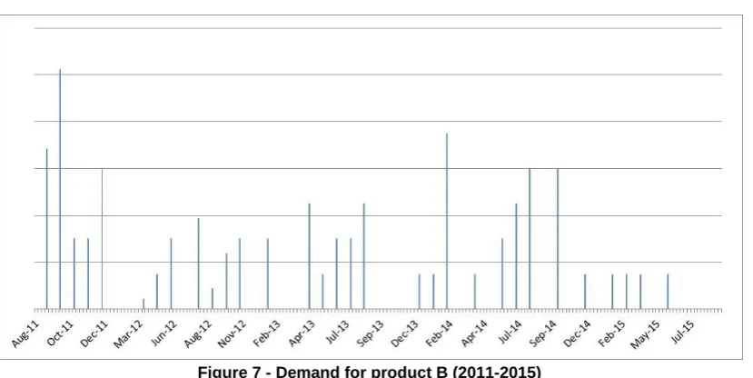
Figure 7 - Demand for product B (2011-2015)

In this figure, we can see that the demand behaviour is quite different from product A. Most of the customers have switched to products that are included with the KEN-LOK® seal. As a result, monthly demand of this product is zero quite often. Products like these have to deal with what is called intermittent demand. This means that demand arrives once every few months.

These two products already show us that it would be wise to set up an APP model to produce a monthly production forecast and analyse required capacities on an aggregated level. Predicting demand for the individual end-products can be very difficult and sensitive to errors. With the APP model, only accumulated demand forecast will be used; which is a lot less sensitive to changes on item level. And so, we will be able to set up a production plan that is a lot more robust.

2.4 Wishes and requirements for the APP model

To try and resolve some of these manufacturing problems via the APP model, we should make sure the APP model reflects the production process of Air Spiralo® as good as possible. Only then, the output of the model is most valuable for the company. Therefore, we will explain the different wishes and requirements for the APP model, which were mentioned by the managers at Air Spiralo® during interviews, in this section.

2.4.1 Planning horizon for APP model

The first thing that should be decided is the preferred length of the planning horizon in the APP model. The planning horizon should consider a pre-defined number of periods, often called time buckets, for which the demand forecast will be given. Since the APP model should consider production on a tactical level, time buckets for APP models are most often equal to months.

(25)

18 2.4.2 Objectives of APP model

The most important aspect of the APP model is the objective function. From the objective function, the model knows what the criteria are for an optimal production plan according to the company.

The managers mentioned that the main goal of the planning model should be to find the lowest possible cost related to realising the forecasted production quantities at Kentel. The total cost should consist of labour and machine production, both by regular and overtime, and also holding cost.

The holding cost should hold two different cost factors. In case that inventory levels stay below the available regular warehouse capacity, the model should apply a pre-defined cost value for the regular warehouse. But as soon as the model plans inventory levels above this capacity, a slightly different cost factor should be applied, because the pallets have to be stored in an extra space. In that extra space, pallets cannot be stored as efficiently as in the regular warehouse and so the holding cost will be higher.

2.4.3 Constraints for APP model

Besides the objective function, the limitations or constraints for the planning model should be defined as well. These constraints should reflect all of the practical limitations present at the manufacturing process at Kentel. Only then, the APP model can search for the correct solution regarding production and inventories.

As we mentioned for the objective function, the inventory levels are allowed to rise above the regular warehouse capacity. The extra items held above the warehouse capacity will be charged with a different cost factor through a step function for the holding costs. Furthermore, the managers at Air Spiralo® mentioned that the APP model should consider the inventory levels as a way of capacity for production. As mentioned in Section 1.1.2, the manufacturing facility Kentel operates, mostly, according to a MTO strategy. Therefore, it does not use inventory such that it can meet demand from on-hand stock, but it can hold inventory for several periods such that less worker capacity is required in periods of high demand.

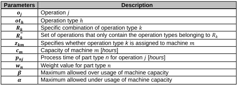
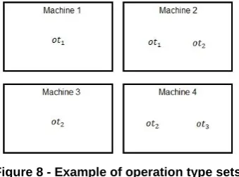
The second preference that became clear from interviews was that the company wants to have an overview of the required capacities for each machine type. The managers want to incorporate the different machine types into the model, because the company is thinking about re-configuring the production lay-out at their manufacturing facilities. It would, therefore, be very useful if the APP model is able to show how much capacity is necessary for each machine type. All these different product groups ask for different machine types. For instance, some products have to go through the seaming process, while others have to go through the ROE process. In total about 35 different process operations are in use at Kentel. We will have to analyse how many of these are required in the APP model.

(26)

19

simply plan overtime production and not hire any extra personnel. By stating this as a hard constraint, we could analyse how much the total costs would decrease if this workers capacity is increased simply via a sensitivity analysis. In that case, the managers can choose for themselves whether it would be beneficial to hire an extra worker, based on this estimated cost decrease.

Furthermore, backlogging is something that the company does not want to allow in a tactical planning model. The company Air Spiralo® is widely known for its reliable delivery; this is how the company distinguishes itself from competitors. Whenever backlogging is created, it should be dealt with during operational planning. Therefore, we should implement a constraint that states that demand must be met at all cost in the specific period. And finally, subcontracting is not an option at Kentel. So again, whenever regular time production and inventory levels are insufficient, it automatically means that overtime production is required.

2.5 Summary

2.5.1 Production planning

In this chapter, we started off by describing how Air Spiralo® manages its organisation regarding production planning. From this description, we can state the following problems regarding production planning at Air Spiralo®,

 Inventory parameters are determined via formulas that have been adapted, based on experience, to the situation at Air Spiralo®; making them very error-sensitive.

 The analysis of productivity showed us that the company is coping with overtime of about 4 FTE on average. Through our APP model, we will analyse whether this is actually the cheapest option for manufacturing or whether it is better to hold items as inventory for some periods.

 The company has to deal quite often with insufficient worker capacity. Implementing the APP model should allow us to analyse the required worker capacity a lot better and act on it, if necessary, by planning overtime or temporarily holding inventory.

 Analysing total demand over the last three years has shown us that demand fluctuates quite a lot around the construction holidays. This will challenge the APP model to plan production optimal even in those periods.

 Demand behaviour can vary a lot between products. Some products are relatively easy to predict, while others are only sold a few months per year. Aggregating products and demand for the APP model should allow us to set up a more reliable production plan on a tactical level.

2.5.2 Wishes and requirements for APP model

In this chapter, we have also described the wishes and requirements, mentioned by the managers, for the APP model. In short, the following wishes and requirements were mentioned,

 The objective of the APP model should be to find the lowest possible total costs that are related to meeting the forecasted demand for Kentel. In the APP model, total costs will consist of production and inventory cost only.

(27)

20

 The APP model should be able to compute required capacities for different kind of machines types.

 Workers cannot be hired or laid-off. Insufficient capacity has to be compensated for via overtime production or holding inventory.

 Finally, subcontracting and backlogging should not be allowed in the APP model. Those options are only considered on operational level.

(28)

21

Chapter 3 Literature review

In this chapter, we will first explain, in Section 3.1, what an APP model does and why it is used. After that, we will perform a literature review in Section 3.2 to try and find articles about APP and other production planning models which allow us to incorporate as many of the wishes and requirements that were mentioned in Chapter 2.

3.1 Aggregate production planning

In 1955, a new production planning model was introduced by the development of the linear decision rule model, also known as HMMS, by Holt and his colleagues (Holt, Modigliani, & Simon, 1955). The introduction of this model started the research and development of aggregate production planning (APP) models. An APP model deals with the process in which a company determines its ideal levels of capacity, production, subcontracting, inventory and stock outs over a specified time horizon for which a demand forecast is given by the use of a linear programming model. The way a linear programming model works is described in Appendix A.1. The planning horizon of an APP model usually consists of 3 to 18 months, but depends on the preferences of the decision maker. The demand forecast is usually based on a rolling horizon in which the forecast is moved forward dynamically.

The APP model is called an aggregate planning model, because it does not plan directly the stock-keeping units (SKUs), but the products on an aggregated level. This aggregation level must be chosen by the decision maker and can be chosen from several possible factors. Some examples of aggregation levels are weight, volume, process stage or process time of the products. For example, if we choose to aggregate products based on their process time, products with similar process times are aggregated into a product group (Chopra & Meindl, 2007).

The APP model finds the optimal solution by varying the decision. A decision variable can state, for example, the amount of planned production, in regular or overtime, of an aggregated product in a specific period. But, a decision variable can also state the inventory levels of the aggregated products at the end of each period. The objective function should reflect the requirements, given by the decision maker, of a good planning. It could be that the APP model should try to find the lowest possible workforce in each period necessary to meet demand, but it could also be that the total cost should be minimised over the whole planning horizon.

In order to find the ideal solution for the aggregate production plan, information is needed that defines the solution space in which the optimal solution exists. This information can consist of relevant costs, process times and/or capacity restrictions. Relevant costs could be production costs, such as labour and transport cost, or the costs for holding inventory. In case of capacity restrictions, one could think of the maximum available machine hours for production in a particular time period. But also restrictions concerning, for example, available overtime for production could be considered.

(29)

22

to the demand in the corresponding time period by laying-off or hiring employees. But if holding inventory is actually cheap and hiring or firing workers is expensive, the model will choose to perform a level strategy. This means that the model will plan the same amount of production during low demand periods to build up inventory in anticipation of future demand. If neither of these strategies will resolve in the optimal value of the objective function, the model will perform a hybrid strategy. This means that the model will follow a mix of both strategies. For instance, the model will choose to only hire or lay-off a few number of employees. Beyond these few number of employees, it becomes too expensive to hire or lay-off workers and the model will perform a level strategy next to it.

3.2 Production models in literature

In this section, we will perform a literature review about APP and other production planning models that involve the wishes and requirements of Air Spiralo®, which we discussed in Section 2.4. If we are able to include as many of these wishes and requirements in our APP model, it will reflect the situation at Air Spiralo® as good as possible. And, as a result, the output of the APP model will be most useful for the company.

During this literature review, we will describe several different articles. In these articles, the researchers are free to define their own abbreviations for decision variables and parameters. As this will create a lot of confusion in our literature review as similar parameters or variables are denoted differently, we will also define our own abbreviations.

3.2.1 Single-objective-single-product APP model

The first requirement, mentioned in Section 2.4, was that we will only have to minimise the total costs regarding production and inventory. These aspects are well reflected by the APP model of Chopra and Meindl (2007). In this book, the researchers developed a basic APP model that aims to minimise the total costs, regarding production, inventory, backlogging and subcontracting costs for a single product(Chopra & Meindl, 2007).

Before the objective function can be formulated, the different decision variables and parameters of the model will have to be defined. In the APP model of Chopra and Meindl (2007), the following decision variables have been defined.

Decision variable Description

𝑷_𝒕 Number of items produced in period 𝑡[units]

𝑶_𝒕 Amount of planned overtime in period 𝑡[hours]

𝑰𝒕 Number of items available in inventory at the end of period 𝑡[units] 𝑩_𝒕 Number of units backlogged at the end of period 𝑡 [units]

𝑪_𝒕 Amount of production outsourced in period 𝑡[units]

𝑾_𝒕 Workforce size in period 𝑡 [units]

𝑯_𝒕 Number of employees hired at beginning of period 𝑡[units]

𝑳_𝒕 Number of employees laid off at beginning of period 𝑡[units]

Table 3 - Decision variables in APP model of Chopra and Meindl (2007)

The first decision variable 𝑃𝑡 states how much is produced in period 𝑡. The second decision

(30)

23

quantities are pushed to the next period and thereby added to the forecasted demand of the next period. Then, the decision variable 𝐶_𝑡 shows how much production is outsourced. So, if regular production time is insufficient, the APP model can choose to create a backlog, plan production in overtime or outsource it to an external producer. Then, in order to state how much regular production time is available, the decision variable 𝑊_𝑡 shows how big the workforce size is. This workforce size can be changed in each period 𝑡 by hiring extra employees via the decision variable 𝐻_𝑡 or firing employees through the decision variable 𝐿_𝑡. Besides these decision variables, the APP model will have to know what the related costs of decision variables or other important factors are. Only then, the APP model can evaluate what the optimal decisions are throughout the planning horizon. These factors are defined via parameters. An overview of the parameters, defined by Chopra and Meindl (2007), can be found in the table below.

Parameters Description

𝒕 Time units in planning horizon T [months]

𝒅_𝒕 Forecasted demand in period 𝑡 [units]

𝒄𝒍𝒓 Production cost in regular time [€/hour]

𝒄𝒍𝒐 Production cost in overtime [€/hour]

𝒄 Inventory holding cost per unit per period [€/unit/month]

𝒃 Backlogging cost per unit per period [€/unit/month]

𝒆 Outsourcing cost per unit [€/unit]

𝒇 Cost to lay off an employee [€/worker]

𝒌 Cost to hire an employee [€/worker]

𝒈 Material cost per unit [€/unit]

𝒓 Amount of items a worker can manufacture in regular time [units/hour]

𝒐 Amount of items a worker can manufacture in overtime [units/hour]

𝒒 Maximum overtime hours allowed per worker [hours/worker]

Table 4 - Parameters in APP model of Chopra and Meindl (2007)

The parameter 𝑑_𝑡 is given as input and states the forecasted demand in period 𝑡. For an APP model, it is assumed that this forecasted demand is deterministic throughout the planning horizon. The parameters 𝑐𝑙𝑟 and 𝑐𝑙𝑜 state how much one worker costs per hour by regular and overtime production respectively. The parameter 𝑐 states how much it costs to keep one unit in stock for a whole month. Then, the parameter 𝑏 states how much it costs to backlog one product into next period. This parameter could be a quantification of the damage to the image of the company by not being able to deliver the customer. Then, the parameter 𝑒

states how much it cost to outsource a product. The parameters 𝑓 and 𝑘 state how much it, respectively, costs to lay-off or hire a worker. The parameter 𝑟 states how many items a worker can manufacture by regular time. This quantity is based on the process time of the product. Next to this parameter, the parameter o states how much a worker can manufacture in overtime production. It could be that, because a worker is not as productive in overtime as in regular production time, this parameter differs significantly from the parameter 𝑟. Then finally, the parameter 𝑞states how many overtime hours are, maximally, allowed per worker each month.

(31)

24

lowest cost will be found by varying the different decision variables for each period. In the end, the objective function is formulated as follows.

𝑀𝑖𝑛 𝑍 = 𝑐𝑙𝑟 ∙ 𝑊_𝑡+ 𝑐𝑙𝑜 ∙ 𝑂_𝑡+ 𝑐 ∙ 𝐼_𝑡+ 𝑏 ∙ 𝐵_𝑡+ 𝑒 ∙ 𝐶_𝑡+ 𝑓 ∙ 𝐿_𝑡+ 𝑘 ∙ 𝐻_𝑡+ 𝑔 ∙ 𝑃_𝑡

𝑇

𝑡=1

1

The next step is to formulate the constraints, which defines the bounds of the solution space for the model. The researchers start off by formulating a constraint regarding the inventory level at the end of each period. This constraint is defined as follows.

𝐼𝑡−1+ 𝑃𝑡+ 𝐶𝑡 = 𝑑𝑡+ 𝐵𝑡−1+ 𝐼𝑡− 𝐵𝑡 𝑓𝑜𝑟 ∀𝑡 2

Here it is stated that the inventory level of previous month plus production, either via own production or what is outsourced, should equal demand plus the backlog of the previous period. If too much production is planned, it can be stored as inventory by the decision variable 𝐼_𝑡. And if too little is produced, a backlog is created via the decision variable 𝐵_𝑡. Furthermore, the APP model should be able to change the workforce size in each period. This is allowed through the following constraint.

𝑊_𝑡 = 𝑊_𝑡−1+ 𝐻_𝑡− 𝐿_𝑡 𝑓𝑜𝑟 ∀𝑡 3

In this constraint, the workforce size of period t is equal to the previous workforce size plus the amount of workers that have been hired in that period minus the amount of workers that have been laid off. Through this constraint, the model can choose to, for example, increase the production capacity by hiring extra workers.

After that, the model has to be forced to plan production in overtime whenever the capacity is still insufficient. To realise this, the decision variables stating the workforce size, the amount of production and overtime hours should be connected to each other. This is done through the following constraint.

𝑃_𝑡 ≤ 𝑟 ∙ 𝑊_𝑡+ 𝑜 ∙ 𝑂_𝑡 𝑓𝑜𝑟 ∀𝑡 4

Here it is stated that the amount which can be produced via regular time, given by 𝑟 ∙ 𝑊_𝑡, plus the amount which can be produced in overtime, given by 𝑜 ∙ 𝑂_𝑡, should give an upper bound to the amount of planned production in period 𝑡.

After that, an upper bound on the number of allowed overtime hours in each period is stated. For this, the following constraint is used.

𝑂_𝑡 ≤ 𝑞 ∙ 𝑊_𝑡 𝑓𝑜𝑟 ∀𝑡 5

This constraint states that only 𝑞 hours per worker may be done by overtime. This is to make sure that, if overtime hours turn out to be the cheapest option, the model does not plan all insufficient capacity through overtime production but also through the other decision variables, such as 𝐶_𝑡.

Finally, since the objective function states that the decision variables should be minimised, it is important to state that the decision variables cannot be negative. Therefore, the final constraint is added as follows.