University of Warwick institutional repository:
http://go.warwick.ac.uk/wrap
A Thesis Submitted for the Degree of PhD at the University of Warwick
http://go.warwick.ac.uk/wrap/54812
This thesis is made available online and is protected by original copyright.
Please scroll down to view the document itself.
2("1
WA~JCK
TESTING FOR UNIT ROOTS AND
COINTEGRATION
IN HETEROGENEOUS PANELS
by
Yuthana Sethapramote
A thesis submitted in partial fulfilment of the
requirements for the degree of
Doctor of Philosophy
In Economics
University of Warwick, Department of Economics
PAGE
NUMBERS
CUTOFF
Table of Contents
Acknowledgements 11 •••••••••••••••••••••••••••••••••••••••••••••••••••••••••••••••••• xi
Declaration of the Author xii
Abstract xiii
1 Introduction and Overview 1
1.1 Motivation 1
1.2 Objectives of the study 7
1.3 Thesis structure 8
2 Unit Root Tests in Heterogeneous Panels
11
2.1 Introduction '" 11
2.2 Literature review 14
2.3 Cross-sectional dependence in panel unit root tests 22
2.4 A Monte Carlo simulation study .32
2.4.1 Simulation design 32
2.4.2 Simulation results : 35
2.5 Unit root tests in a mixed panel of stationary and non-stationary series .44
2.6 The effect of cross-sectional dependence 48
2.7 Unit root tests in cross-correlated panels 55
2.7.1 Bootstrapping panel unit root tests 55
2.7.2 Unit root tests with seemingly unrelated regression 60
2.7.3 Panel unit root tests with a factor model.. , 64
2.8 Conclusion " 70
3 Cointegration tests in heterogeneous panels
73
3.1 Introduction 73
3.2 Literature review 76
3.3 The panel data cointegration tests 82
3.3.2 The likelihood-based panel cointegration tests 83
3.4 A Monte Carlo simulation study 86
3.4.1 Simulation design 86
3.4.2 Simulation results 92
3.5 Cointegration tests in a mixed panel of cointegrated and non-cointegrated
relationships 102
3.6 Bootstrapping panel cointegration tests 106
3.6.1 Bootstrapping residual-based test.. 106
3.6.2 Bootstrapping likelihood-based test.. 108
3.6.3 Monte Carlo results 110
3.7 Panel cointegration test with a factor model , 114
3.8 Conclusion 116
4 Panel Unit Root
Tests
with StructuralBreaks ••.•••...•.••..•...•...•...
118
4.1 Introduction 118
4.2 Literature review 122
4.3 Panel unit root tests allowing for structural breaks 129
4.3.1 The panel LM unit root test without breaks 130
4.3.2 The exogenous break panel LM unit root test.. 132
4.3.3 The endogenous break panel LM unit root test.. 133
4.4 Monte Carlo experiments on the panel LM unit root test without shifts .136
4.3.1 The finite sample size and power 137
4.3.2 Simulations with a mixture of stationary and non-stationary series
in the panel 140
4.3.3 The effect of cross-sectional dependence 142
4.5 Monte Carlo experiments on the exogenous break panel LM unit root test...146
4.5.1 Experiments on the exogenous break test when the break points are
correctly specified 147
4.5.2 Experiments on the exogenous break test when the number of
breaks is over- and under-specified 148
4.5.3 Experiments on the exogenous break test when the location of
4.6 Monte Carlo experiments on the endogenous break panel LM
unit root test 157
4.6.1 The finite sample means and variances .158
4.6.2 The accuracy of estimating the true break points 165
4.6.3 The finite sample size and power. 171
4.7 Conclusion 182
5
Panel Evidence on Fundamental Exchange Rate Modelling from Asia
Pacific Countries 184
5.1 Introduction 184
5.2 Literature review 188
5.3 Purchasing power parity and the monetary approach to exchange rate
modelling 195
5.3.1 Purchasing power parity 195
5.3.2 The monetary approach to exchange rate modelling 197
5.4 Empirical results 201
5.4.1 Data 201
5.4.2 Empirical results of the single country time-series Data 203
5.4.3 Empirical results of the panel data test 221
5.5 The impact of the 1997 East Asian currency crisis 226
5.5.1 Empirical results using the sample period before the 1997 crisis 226
5.5.2 Empirical results from the exogenous-break LM unit root tests 233
5.5.3 Empirical results from the endogenous-break LM unit root tests 235
5.6 Conclusion '" 241
Appendix A 244
6
Conclusion and Directions for future research
246
6.1 Concluding remarks 246
6.2 Directions for future research 252
List of Figures
Chapter 2
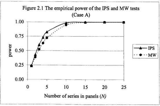
Figure 2.1 The empirical power of the IPS and MW tests (Case A) 41
Figure 2.2 The empirical power of the IPS and MW tests (Case B) 41
Figure 2.3 The empirical power of the IPS and MW tests in a mixed panel, when N =5 .45 Figure 2.4 The empirical power of the IPS and MW tests in a mixed panel, when N =25 .45 Figure 2.5 The empirical power of the IPS and MW tests in a mixed panel, when N
=
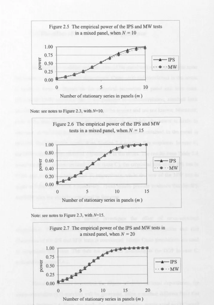
10 47Figure 2.6 The empirical power of the IPS and MW tests in a mixed panel, when N
=
15 47Figure 2.7 The empirical power of the IPS and MW tests in a mixed panel, when N=20 .47
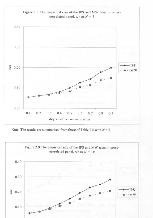
Figure 2.8 The empirical size of the IPS and MW tests in cross-correlated panel, when N
=
5 50Figure 2.9 The empirical size of the IPS and MW tests in cross-correlated panel, when N=10 50
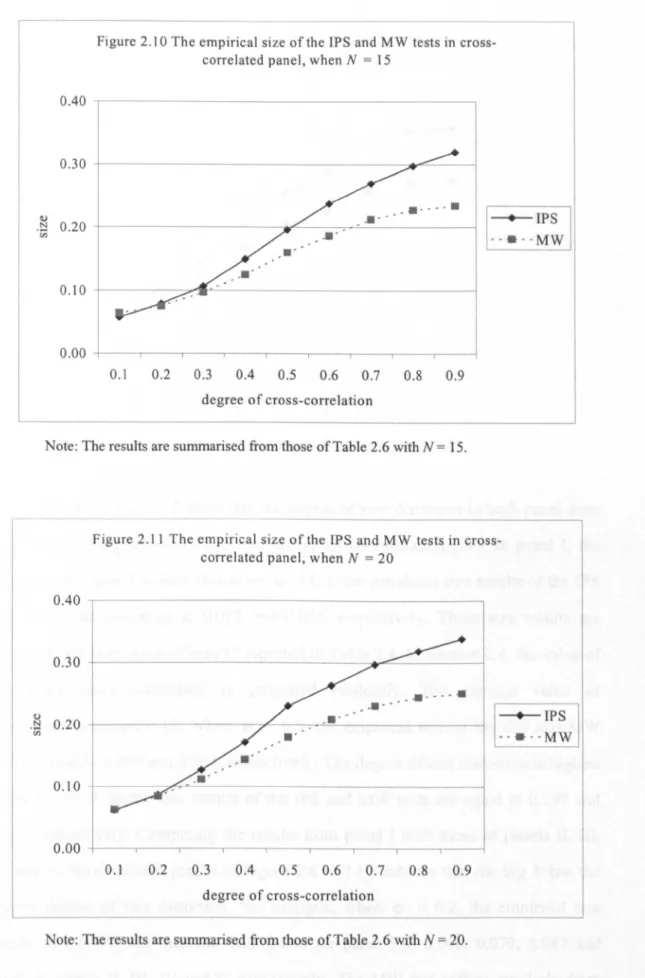
Figure 2.10 The empirical size of the IPS and MW tests in cross-correlated panel, when N
=
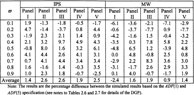
15 51 Figure 2.11 The empirical size of the IPS and MW tests in cross-correlated panel, when N=
20 51 Figure 2.12 The empirical size of the IPS and MW tests in cross-correlated panel, when N=
25 52Figure 2.13 The empirical power of the CIPS* test (Case A and B) 66
Chapter
3
Figure 3.1 The empirical power of panel cointegration tests in a mixed panel, when k=2, N=5 103
Figure 3.2 The empirical power of panel cointegration tests in a mixed panel, when k=3, N=5 103
Figure 3.3 The empirical power of panel cointegration tests in a mixed panel, when k=2, N=10 103
Figure 3.4 The empirical power of panel cointegration tests in a mixed panel, when k=3, N=10 104
Figure 3.5 The empirical power of panel cointegration tests in a mixed panel, when k=2, N=15 104
Figure 3.6 The empirical power of panel co integration tests in a mixed panel, when k=3, N=15 104
Chapter 4
Figure 4.1 The empirical power of the panel LM and IPS tests 138
Figure 4.2 The empirical power of the panel LM and IPS tests in a mixed panel of stationary and
non-stationary series in the case of small panel (N=5) 141
Figure 4.3 The empirical power of the panel LM and IPS tests in a mixed panel of stationary and
non-stationary series in the case of large panel (N=25) , 141
Figure 4.4 The empirical size of the panel LM and IPS tests in cross-correlated panel, when N=S 143
Figure 4.5 The empirical size of the panel LM and IPS tests in cross-correlated panel, when N=10 .. 144
Figure 4.6 The empirical size of the panel LM and IPS tests in cross-correlated panel, when N=15 .. 144
Figure 4.7 The empirical size of the panel LM and IPS tests in cross-correlated panel, when N=20 .. l45
Chapter
5
Figure 5.1 Nominal exchange rates (Si,t) in Asia Pacific countries 204
Figure 5.2 Price levels (Pi,t) in Asia Pacific countries 205
Figure 5.3 Relative money supplies (m;,/) in Asia Pacific countries 206
Figure 5.4 Relative real incomes (Y;,t ) in Asia Pacific countries 207
Figure 5.5 Real exchange rates (qi,t) in Asia Pacific countries 209
List of Tables
Chapter
2
Table 2.1 Matrix of cross-correlation (n )used in the DGP in case C 34
Table 2.2 The empirical power of the standard ADF test 36
Table 2.3 The empirical size and size-adjusted power of the standard ADF test under the null and
alternative hypotheses of the IPS and MW tests 37
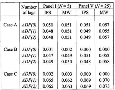
Table 2.4 The empirical size of the IPS and MW tests 39
Table 2.5 The empirical power of the IPS and MW tests 39
Table 2.6 The empirical size of the IPS and MW tests in cross-correlated panels 49
Table 2.7 The empirical size of the IPS and MW tests in cross-correlated errors panels using the
ADF(S) specification 53
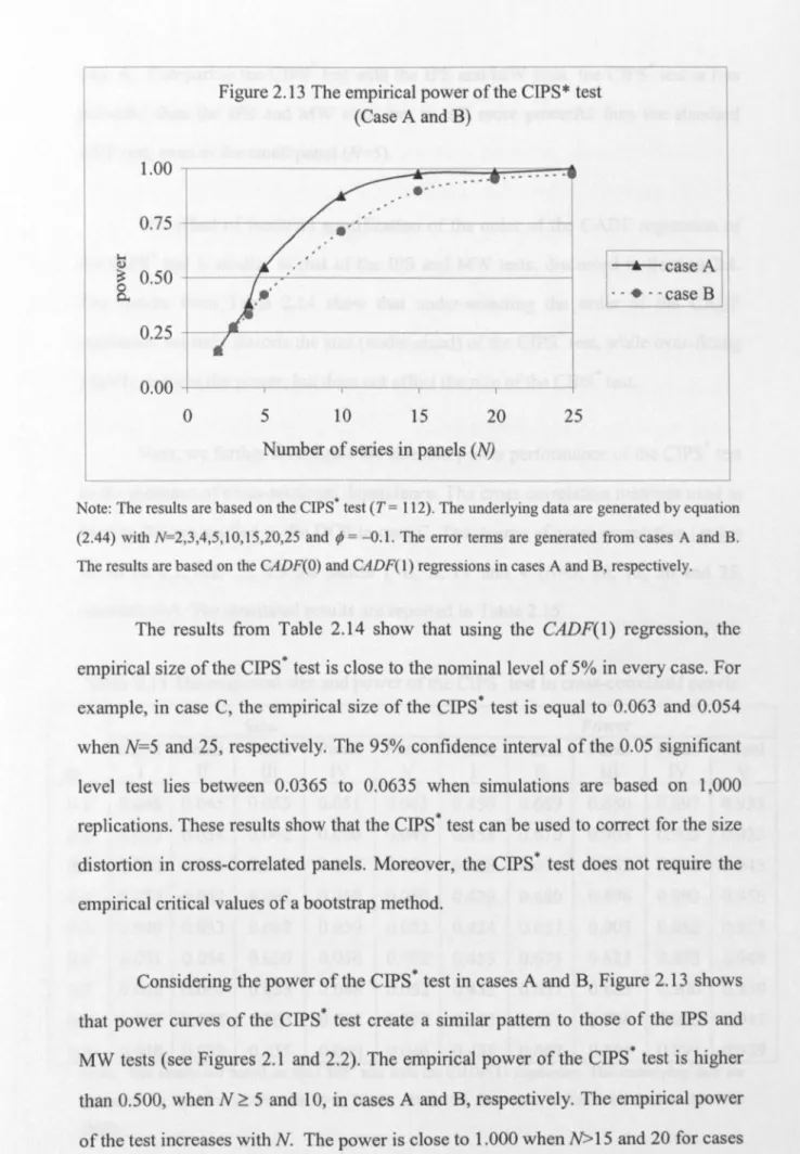
Table 2.8 The percentage differences between the empirical size of the IPS and MW tests estimated
with the ADF(1) and ADF(S) regressions 53
Table 2.9 The estimated cross-correlation matrix in the PPP data reported in Bornhorst (2003) 5(5
Table 2.10 The empirical size of the bootstrap IPS and MW tests 57
Table 2.11 The empirical power of the bootstrap IPS and MW tests 58
Table 2.12 The empirical size and power of the SURADF test 6~
Table 2.13 The empirical size and power of the SURIPS test
62
Table 2.14 The empirical size and power of the CIPS· tests 65
Table 2.15 The empirical size and power of the CIPS· test in cross-correlated panels 67
Chapter 3
Table 3.1 The estimated cross-correlation matrix of the OLS residuals from a monetary exchange
rate model reported in Groen (2000) 91
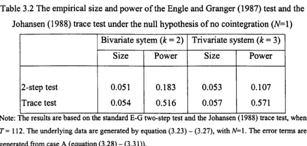
Table 3.2 The empirical size and power ofthe Engle and Granger (1987) test and the
Johansen (1988) trace test under the null hypothesis of no cointegration (N=1) 93
Table 3.3 The empirical size, power and size-adjusted power of the standard Engle and
Granger (1987) two-step test and Johansen (1988) trace test when the same null and
alternative hypotheses as those of the panel cointegration tests (N=5) are applied 9~
Table 3.4 The empirical size and power of the panel cointegration tests in the bivariate system,
when N=S 9S
Table 3.5 The empirical size and power of the panel cointegration tests in the trivariate system,
when N=10 96
Table 3.6 The empirical size and power of the panel cointegration tests in the bivariate system,
Table 3.7 The empirical size and power of the panel co integration tests in the trivariate system,
when N=10 99
Table 3.8 The empirical size and power of the panel cointegration tests in the bivariate system,
when N=15 100
Table 3.9The empirical size and power of the panel cointegration tests in the trivariate system,
when N=15 100
Table 3.10 The empirical power of the panel cointegration tests in a mixed panel (N=5) 102
Table 3.11 The empirical size and power of the bootstrap panel cointegration tests in the
bivariate system 111
Table 3.12 The empirical size and power of the bootstrap panel cointegration tests in the
trivariate system 111
Table 3.13 The empirical size and power of the residual-based panel co integration test ofCIPS
in the bivariate and trivariate systems 114
Chapter 4
Table 4.1 The empirical size and power of the panel LM unit root test. 138
Table 4.2 The empirical size of panel LM test in the panel with cross-correlated errors estimated
using the LM( 1) and LM(5) regression 143
Table 4.3 The empirical size of the exogenous break panel LM unit root test , 147
Table 4.4 The empirical power of the exogenous break panel LM unit root test. 148
Table 4.5 The empirical size and power of the exogenous one- and two-break panel unit root test
when there is no break in the DGP 149
Table
4.6
The empirical size and power of the exogenous two-break panel unit root test whenthere is one break in the DGP 149
Table 4.7 The empirical size of the panel LM test (without shifts) and the IPS test (without shifts)
when there are one- or two- breaks in the DGP 150
Table 4.8 The empirical power of the panel LM test (without shifts) and the IPS test (without shifts)
when there are one- or two- breaks in the DGP 150
Table 4.9 The empirical size of the exogenous one-break panel LM unit root test when there are
two breaks in the DGP 151
Table 4.10 The empirical power of the exogenous one-break panel LM unit root test when there
are two breaks in the DGP 152
Table 4.11 The empirical size of panel LM test when the break points is incorrectly specified 154
Table 4.12 The empirical power of panel LM test when the break points is incorrectly specified 155
Table 4.13 Means of the endogenous one-break LM unit root test with different magnitude of
break .159
Table 4.14 Means of the endogenous one-break LM unit root test with different location of
Table 4.15 Variances of the endogenous one-break LM unit root test with different magnitude
of break 160
Table 4.16 Variances of the endogenous one-break LM unit root test with different location
of break 160
Table 4.17 Means of the endogenous two-break LM unit root test with different magnitude
of break 161
Table 4.18 Means of the endogenous two-break LM unit root test with different location
of break 161
Table 4.19 Variances of the endogenous two-break LM unit root test with different magnitude
of break 162
Table 4.20 Variances of the endogenous two-break LM unit root test with different location
of break 162
Table 4.21 The accuracy of estimating the true break point of the endogenous one-break LM
unit root test (under the null hypothesis) 166
Table 4.22 The accuracy of estimating the true break point of the endogenous one-break LM
unit root test (under the alternative hypothesis} 167
Table 4.23 The accuracy of estimating the true break point of the endogenous two-break LM
unit root test (under the null hypothesis} 168
Table 4.24 The accuracy of estimating the true break point of the endogenous two-break LM
unit root test (under the alternative hypothesis) 169
Table 4.25 The empirical size of the endogenous one- and two-break min-tp panel LM
unit root test 171
Table 4.26 The empirical size of the endogenous one- and two-break max-I
to
I panel LMunit root test 172
Table 4.27 The empirical size of the endogenous one- and two-break min-SRC panel LM
unit root test 172
Table 4.28 The empirical power of the endogenous one- and two-break min-tp panel LM
unit root test 172
Table 4.29 The empirical power of the endogenous one- and two-break max-I
to
I panel LMunit root test 173
Table 4.30 The empirical power of the endogenous one- and two-break min-SRC panel LM
unit root test 173
Table 4.31 The empirical size of the endogenous break
min-t
p panel LM unit root test usingadjustment parameters from the endogenous-break test without shifts 176
Table 4.32 The empirical size of the endogenous break max-I
to
I panel LM unit root test usingadjustment parameters from the endogenous-break test without shifts 176
adjustment parameters from the endogenous-break test without shifts 177
Table 4.34 The empirical power of the endogenous break
min-t
p panel LM unit root test usingadjustment parameters from the endogenous-break test without shifts 177
Table 4.35 The empirical power of the endogenous break max-I
tt5
I panel LM unit root test usingadjustment parameters from the endogenous-break test without shifts 177
Table 4.36 The empirical power of the endogenous break min-SBC panel LM unit root test using
adjustment parameters from the endogenous-break test without shifts 178
Table 4.37 The empirical size of the endogenous break min-
t
p panel LM unit root test usingadjustment parameters from the exogenous-break test 178
Table 4.38 The empirical size of the endogenous break max-I
tt5
I panel LM unit root test usingadjustment parameters from the exogenous-break test 179
Table 4.39 The empirical size of the endogenous break min-SBC panel LM unit root test using
adjustment parameters from the exogenous-break test 179
Table 4.40 The empirical power of the endogenous break min-
t
p panel LM unit root test usingadjustment parameters from the exogenous-break test 180
Table 4.41 The empirical power of the endogenous break max-I
tt5
I panel LM unit root test usingadjustment parameters from the exogenous-break test 180
Table 4.42 The empirical power of the endogenous break min-SBC panel LM unit root test using
adjustment parameters from the exogenous-break test 180
Chapter 5
Table 5.1 The sample spans and seasonal adjustment property of the real income data in Asia
Pacific countries 202
Table 5.2 The ADF results for the level of series 212
Table 5.3 The ADF results for the first difference ofseries 213
Table 5.4 Empirical results of the ADF tests for the level of real exchange rates (qi.,) and
deviations from monetary fundamental (Zi.') 213
Table 5.5 Empirical results of the ADF tests for the first difference of real exchange rates(qi.,)
and deviations from monetary fundamental (zi.t)' 214
Table 5.6 Empirical results of the LM tests for the level of real exchange rates (qi.,) and
deviations from monetary fundamental (Zi.') 214
Table 5.7 The estimated cross-correlation matrix of the residuals from the ADF regressions for
Table 5.8 The estimated cross-correlation matrix ofthe residuals from the ADF regressions for
deviations from monetary fundamental (Zi.t) 216
Table 5.9 Empirical results of the SURADF tests for real exchange rates (qi,t) and deviations
from monetary fundamental (Zi,t)" 218
Table 5.10 The Engle-Granger and Johansen likelihood-ratio test results for the PPP hypothesis 220
Table 5.11 The Engle-Granger and Johansen likelihood-ratio test results for the monetary model. 220
Table 5.12 Panel unit root test results for real exchange rates (qi,I) 222.
Table 5.13 Panel unit root test results for deviations from monetary fundamental (Zi,t) 22~
Table 5.14 Panel cointegration test results for the PPP hypothesis 224
Table 5.15 Panel cointegration test results for the monetary model
224-Table 5.16 Empirical results of the ADF tests for real exchange rates (qi,t )and deviations from
monetary fundamental (Zj,t) in the pre-crisis period 227
Table 5.17 Empirical results of the LM tests for real exchange rates (qi.l) and deviations from
monetary fundamental (zj,l) in the pre-crisis period 22
Table 5.18 Empirical results of the SURADF tests for real exchange rates (qj,t ) and deviations
from monetary fundamental (Zi.t) in the pre-crisis period 22.
Table 5.19 The Engle-Granger and Johansen likelihood-ratio test results for the PPP hypothesis
in the pre-crisis period , 23
Table 5.20 The Engle-Granger and Johansen likelihood-ratio test results for the monetary
model in the pre-crisis period 23
Table 5.21 Panel unit root test results for the PPP hypothesis and the monetary model in
the pre-crisis period 23
Table 5.22 Panel cointegration test results for the PPP hypothesis and the monetary model in
the pre-crisis period 23
Table 5.23 Empirical results of the exogenous break LM unit root test for real exchange
rates (qj,t) and deviations from monetary fundamental (Zj,t) ·
23
Table 5.24 Empirical results of the endogenous break min-tp LM unit root test for real
exchange rates (qj,t) and deviations from monetary fundamental (Zj,t) ..
···23
Table 5.25 Empirical results of the endogenous break max-I
to
I LM unit root test for realexchange rates (qj,t )and deviations from monetary fundamental (zj,t)' 2~
Table 5.26 Empirical results of the endogenous break min-SBC LM unit root test for real
Acknowledgements
Iam grateful to numerous people who have contributed to the shaping of this thesis. At the
outset, I would like to express my appreciation to my supervisors, Mike Clement, for his
guidance, patience and encouragement throughout my PhD study at Warwick, and Jeremy
Smith for his encouragement and helpful advice since my MSc study and throughout my
PhD research. His MSc time-series analysis class has had a significant influence on my
research and future career.
I would also like to acknowledge many other colleagues: P'Mee, P'Pong, May, Prem,
Pedro, Tong, Cherry, Kay, Mimi and Pim, for their help and support in many ways during
my study at Warwick.
Financial support provided by the Royal Thai Government Scholarship is gratefully
acknowledged.
Declaration of the Author
I declare that this thesis is my own work and has not been submitted for a degree in
another university.
No material contained in this thesis has been previously published.
Yuthana Sethapramote
January 21, 2005
Abstract
This thesis undertakes a Monte Carlo study to investigate the finite sample properties of several
panel unit root and cointegration tests. To this end, we consider a number of different experiments
which potentially affect the properties of the tests.
We first consider panel unit root tests in heterogenous panels. Application of the panel tests of Im,
Pesaran and Shin (2003) (IPS), and Maddala and Wu (1999) (MW) increases their power over the
standard ADF test. However, the power of the tests is significantly diminished when the panel is
dominated by the non-stationary series. Neglecting the presence of cross-sectional dependence
results in serious size distortions. In view of this, a variety of methods are applied to correct the size
distortions. However, the power of all tests is diminished as the cross-correlations reduce the amount
of independent information in the panel.
The simulation results from the panel cointegration tests extend the findings of the unit root tests to
multivariate cases. The likelihood-based panel rank test of Larsson, Lyhagen and Lothgren (2001) is
found to be more powerful than the residual-based panel tests of IPS and MW, but slightly
over-sized in moderate sample sizes (Z). The effects of a mixed panel and of cross-correlations in the
errors are similar to those of panel unit root tests. Therefore, we again, use the bootstrap method and
the Cross-sectionally augmented IPS test (CIPS) ofPesaran (2003) to correct the size distortions.
The presence of structural breaks affects the size and power properties of any panel unit root tests
which fail to cope with it. When the break dates are known, the exogenous break panel LM test is
applied, to control the effect of structural shifts. In addition, the endogenous break selection
procedures are used to estimate the break points. The endogenous break panel LM test also
performs considerably well in terms of the size, power and accuracy with which the true break
points are estimated.
Finally, application of the panel unit root and cointegration tests provide some evidence in support of
the existence of long-run PPP and the monetary model in Asia Pacific countries. In addition, the
presence of structural breaks as the impact of the currency crisis is also detected. However, evidence
is found to be sensitive to the choice of deterministic terms (intercepts, trends), the methods used to
Chapter 1
Introduction and Overview
1.1 Motivation
Standard unit root (cointegration) tests have limited power to reject the null
hypothesis of non-stationarity (no cointegration) when the underlying process is
highly persistent. The problem of low power is particularly severe in small samples
(see Lothian and Taylor (1997), and Maddala and Kim (1999». Recently, there has
been a surge of interest in the adding of information from the cross-section
dimension to form panels, in order to investigate the effect of this additional
information on the performance of both unit root and cointegration tests. Various
panel unit root and cointegration tests have been proposed, based on macro-panels
with both large N (cross-section dimension) and T(length of time-series). Interms of characteristics, these large N,large Tpanels differ from the traditional large N,small
T panels. When T is large, there is an obvious need to address issues of
non-stationarity in the data.
Panel unit root tests gained popularity with the tests introduced by Quah
(1994), Levin, Lin and Chu (2002) (henceforth, LLC), Im, Persasan and Shin (2003)
(henceforth, IPS), Maddala and Wu (1999) (henceforth, MW), and Choi (2001).
opportunity to increase the power of the unit root tests using data from the
cross-section dimension. LLC construct a unit root test for homogeneous panels based on
the Augmented Dickey-Fuller (ADF) t-statistics constructed from the sample pool
estimator with some modifications. However, this homogeneity assumption is very
restrictive. The main disadvantage of this approach is that differences in adjustment
speeds and dynamics across cross-sectional units are not taken into account.
Alternatively, IPS and MW propose panel unit root tests for heterogeneous panels.
The panel IPS test is calculated from the average t-statistic of the individual ADF
regressions. The z-bar statistic is then adjusted, using its mean and variance. This
standardised IPS statistic is asymptotically distributed as a standard normal.
Similarly, the panel MW test is calculated from the p-values of the individual unit
root tests, and has a standard chi-square distribution. These panel unit root tests
provide researchers with the advantage of increasing the dimension from the
individual unit root tests, while still allowing for heterogeneity of the individual
series in the panel.
The panel data methodology has been further extended to test for
cointegration relationships. There are two main approaches
inthe literature on
cointegration analysis within panels. The first approach is a panel version of the
Engle and Granger (1987) residual-based two-step cointegration test.
Inthis
approach, a long-run relationship is estimated in the first step.
Inthe second step, a
test for the existence of unit roots on the residuals obtained from the long-run
regressions based on the ADF regressions is constructed. Kao (1999) develops a
number of variants of the residual-based panel cointegration tests based on a
homogeneity assumption. Pedroni (1999) introduces a number of panel cointegration
statistics based on both homogeneity and heterogeneity assumptions.
Inaddition,
heterogeneous panel cointegration tests can be estimated, using the panel IPS and
MW unit tests on the residuals from the long-run regressions. The second approach
cointegration rank in a VAR of Johansen (1988). Larsson, Lyhagen and Lothgren
(2001) (henceforth, LLL) develop a panel test for determining cointegrating rank in
the long-run
n
matrix as the average of the individual likelihood-basedcointegration rank trace test statistics. This LLL
LR-bar
statistic, defined similarly asthe IPS
z-bar
statistic, is also based on heterogeneous panels.There remains a number of concerns regarding the testing for unit roots and
cointegration in panel data. First, MW make reference to the case where there is a
mixture of stationary and non-stationary series in the groups as an alternative
hypothesis. Theoretically, in heterogeneous panels, the null hypothesis of
non-stationarity can be rejected when there is at least one stationary series in the panel.
However, the power of any panel test may drop significantly in a mixed panel
dominated by non-stationary series. Second, the properties of the panel test statistics
are based on the assumption that the error terms in each cross-section are
independent. The effect of cross-sectional dependence has been discussed in several
papers (see O'Connell (1998) and Cerrato (2001». In cross-country data, the presence of cross-sectional correlation is likely to arise, due to the existence of
inter-economy linkages. However, the presence of cross-sectional dependence in the error
terms means that the limit distributions of the panel unit root and cointegration tests
are no longer valid. O'Connell (1998) points out that the panel unit root tests that
neglect the cross-sectional correlation can be seriously over-sized. Inaddition, even if the true distribution of the test statistic are available, the power of the test
decreases as the total amount of independent information contained in the panel is
reduced.
Recently, several methods have been proposed to control for the effect of
cross-sectional dependence in the panel unit root tests. IPS suggest removing the
effect of the common time-specific components by subtracting the cross-sectional
procedure is valid only in the case of homogeneous cross-sectional dependence, and
is not robust if the time-specific components vary across the groups. Alternatively,
MW recommend a bootstrap procedure to calculate the empirical distribution of the
test statistic to compensate for the size distortions of the conventional IPS and MW
tests in cross-correlated panels. Finally, Pesaran (2003) introduces a
Cross-sectionally augmented IPS test (CIPS), which approximates the structure of error
correlation by a factor model. This CIPS test applies the standard ADF regressions
augmented with the cross-section average of lagged levels and first-differences of the
individual series.
Another issue, which had generated wide-ranging discussion in the unit root
literature in the last decade, is the presence of structural changes in time-series data.
Testing for unit roots, allowing for possible structural breaks, has received
considerable attention since the pioneering work of Perron (1989). A shift in the
intercept and/or the trend function of a stationary time-series reduces the power of
standard unit root tests (see Perron (1989». Recently, standard unit root tests have
been adjusted to discriminate between the existence of a unit root process and a
stationary process with structural instability. Perron (1989, 1990) proposes a
modified ADF test to allow for a structural shift, by including a relevant dummy
variable in the ADF regression. In these papers, the break point is assumed to be
exogenously given. An endogenous break selection method has been developed
subsequently by Zivot and Andrews (1992), Banerjee
et al.
(1992), and Perron andVogelsang (1992), to determine the break point from the data. The most widely used
endogenous selection procedure is the minimum test, which selects the break date by
minimising the t-statistic for testing unit roots.
Inthe panel data framework, one would expect the existing panel unit root tests, such as the IPS and MW tests, to suffer from a significant loss of power in the
for structural breaks, has been widely documented in the literature, panel unit root
tests with structural shifts have not received much attention. The main difficulty in
the application of structural changes in panel data is that the asymptotic property of
Perron-type ADF t-statistics varies according to the location of breaks in the series.
The expected values and variances of the ADF
t-statistics
at all different possiblelocations of breaks in the sample are then required in computing the IPS-type panel
unit root test with structural breaks. Therefore, the calculation of these statistics is
practically unmanageable.
Recently,
1m,
Lee and Tieslau (2002) (henceforth, ILT) have developed anew panel unit root test based on the Lagrangian Multiplier (LM) principle, which is
a panel version of the LM unit root test of Amsler and Lee (1995). This LM unit root
test has the same asymptotic distribution as that of the LM test without a shift,
originally presented by Schmidt and Phillips (1992). The asymptotic distribution of
this test does not depend on the nuisance parameters that indicate the position of a
structural shift. ILT show that this invariance property of the univariate LM unit root
test is still valid in their proposed panel LM unit root test. The panel LM test with a
level shift can use the same means and variances that apply to the panel LM test
without a shift. Moreover, this invariance property is also useful in constructing the
tests based on heterogeneous panels. The panel LM unit root test can be applied
when more than one structural shift occurs, or when structural shifts in each
cross-section unit occur at different locations.
However, the ILT panel LM unit root test assumes that the number and
location of breaks are accepted as a priori. Lee and Strazicich (2003) propose a
univariate minimum LM unit root test, which extends the LM unit root test of Amsler
and Lee (1995) to allow for the unknown break points that are determined
endogenously from the data. The endogenous break LM test of Lee and Strazicich
Andrews (1992). The break points are selected to minimise the t-statistics used to test
for the unit root null hypothesis. Lee and Strazicich (2003) show that the asymptotic
property of this minimum LM unit root test does not depend on the location of breaks
under the null hypothesis. This endogenous break selection procedure provides the
method to determine the presence and the location of breaks from the data, which is
practically useful.
Recently, a number of empirical researchers have applied panel unit root and
co integration tests to investigate several key economic issues, for example, growth
and convergence (see Evans and Karras (1996) and Lee, Pesaran and Smith (1997»
and international R&D spillovers (see Kao, Chiang and Chen (1999». However, the
empirical study to have generated the greatest attention is in the field of fundamental
exchange rate modelling. The standard economic theories that are widely used to
explain the exchange rate movements are purchasing power parity (PPP) and the
monetary model. Empirical research on exchange rates and their fundamental
determination yields controversial results regarding the ability of fundamental
economic factors to explain exchange rate movements (see Rogoff (1996) and Taylor
(1997». The failure to find favourable evidence in support of the PPP hypothesis and
the monetary model is explained as a result of the low power of standard unit root
and cointegration tests. Lothian and Taylor (1997) argue that the standard ADF test
has extremely low power in rejecting the unit root null hypothesis for real exchange
rates over the post-Bretten Woods sample period. Therefore, panel data analysis has
been applied to improve the results over the conventional individual time-series
analysis. Recently, several articles, such as Frankel and Rose (1996), Wu (1996),
Papell (1997), and Coakley and Fuertes (1997) have found evidence to support PPP
with regard to panel data, while Oh (1999) and Groen (2000) find positive results for
Even though a number of empirical studies on exchange rate determination
using panel data find evidence to validate PPP and the monetary model, these studies
usually focus on industrial DECD countries. For less-developed countries, empirical
evidence is still not widely investigated. The importance of Asia Pacific countries
has rapidly increased in the last two decades with the rapid economic growth and
strong trading ties to the world economy. In 1997, the Asia Pacific region was
strongly affected by a severe currency crisis, which forced most countries to change
their exchange rate regimes and implement structural economic reforms. The validity
of the PPP hypothesis and the monetary model in the region has been applied in
studies on the cause and impact of the currency crisis (see, for example, Chin (2000)
and Razzaghipour et al. (2001».
The effect of the 1997 East Asian crisis is a major concern for the testing of
unit roots in real exchange rates and deviations from monetary fundamental. The
crisis is likely to have produced a structural shift, which should be taken into account
in testing for unit roots. For this reason, the panel LM unit root test of ILT is useful
in modelling exchange rate movements in Asia Pacific countries. Inthis framework, the impact of the 1997 crisis and the low power of the individual unit root tests can
be addressed, using the panel unit root test with structural shifts.
1.2 Objectives of the study
In light of the above discussion, the objectives of the thesis are to build on
and extend the research in the field of panel data techniques applied to unit root and
Evaluating the finite sample performance of several panel unit root and
cointegration tests in terms of the size and power, when the length of
time-series is moderate and the speed of adjustment in a mean-reverting
process is quite slow.
Examining the effect of a mixed panel of stationary and non-stationary
series and the impact of cross-sectional dependence on the size and power
properties ofthe panel tests.
Comparing alternative methods for testing unit roots and cointegration in
cross-correlated panels.
Investigating the effect of structural breaks on the size and power
properties of the panel unit root tests, both when the shifts are allowed
and when they are neglected.
Applying the panel unit root and cointegration tests in an empirical
investigation into the presence of a long-run relationship between
exchange rates and their fundamentals in Asia Pacific countries, and the
impact of the 1997 East Asian currency crisis.
1.3 Thesis structure
The content of the thesis falls into four overall categories: panel unit root
tests, panel cointegration tests, panel unit root tests with structural breaks, and an
empirical investigation of exchange rates and their fundamentals in Asia Pacific
In Chapters 2 to 4, the main methodology applied in the studies is Monte
Carlo simulations. This method is used to investigate the finite sample properties of
several panel unit root and cointegration tests in heterogeneous panels. The
simulation results are used to compare the size and power performance of the tests,
based on a number of different experiments.
Chapter 2 examines the panel unit root tests of IPS and MW. We focus on the
improvement in the power of the panel unit root tests over the standard individual
time-series tests. In addition, two concerns in testing for unit roots in heterogeneous
panels are addressed. First, the effect of having a mixture of both stationary and
non-stationary series in the panel is considered. Second, the impact of cross-sectional
dependence is investigated. For cross-sectional dependence, we examine the
performance of the three methods for the testing of unit roots in cross-correlated
panels: the bootstrap method, the Seeming Unrelated Regression (SUR) and the
Cross-sectionally augmented IPS test (CIPS).
Chapter 3 focuses on the panel cointegration tests. The panel unit root tests of
IPS and MW are applied to test for cointegration relationships based on the
residual-based methodology of Engle and Granger (1987). In addition, we investigate the
panel cointegration test of LLL, which applies the method testing for the
cointegration rank in a VAR of Johansen (1988) to the panel data framework. We,
again, consider the effect of having a mixture of cointegrated and non-cointegrated
relationships in the panel and of cross-sectional dependence. The bootstrap method
and the CIPS test are applied to control for the effect of cross-correlation in the
residual-based and likelihood-based panel cointegration tests.
Chapter 4 investigates the effect of structural breaks in testing for unit roots
power properties of the standard panel IPS and LM unit root tests without shifts, as
well as the panel LM unit root test of ILT. We evaluate the performance of the tests
when the break points are exogenously determined and assumed to be a priori. Next,
we apply the endogenous selection procedures to estimate the break points. The finite
sample performance of the endogenous break panel LM unit root test is investigated
in terms of the size, power and accuracy of selecting the true break dates.
In Chapter 5, we investigate the empirical evidence for a long-run
relationship between exchange rates and their fundamentals in Asia Pacific countries.
The PPP hypothesis and the monetary model are used as the fundamental
determination of exchange rate movements. Several of the panel data methods
analysed in Chapters 2 to 4 are then applied to an empirical investigation of long-run
PPP and the monetary model. Inaddition, we address the impact of the 1997 East Asian currency crisis. The presence of a structural break, due to the aftermath of the
currency crisis is considered in exchange rate modelling.
Chapter 6 concludes the thesis with a summary of the way in which the
research objectives have been investigated. The contributions of the thesis to panel
data unit root and co integration testing are noted, as well as some possible
Chapter 2
Unit Root Tests in Heterogeneous Panels
2.1 Introduction
Testing for unit roots in panel data has attracted much attention in recent
literature, and various statistics for testing such data have been proposed. Panel unit
root tests have gained popularity since the pioneering papers of Quah (1994), and
Levin, Lin and Chu (2002) (LLC). However, their tests are based on a homogeneity
assumption, in which the autoregressive coefficients are the same across the
individual series in the panel. This assumption is quite restrictive, implying identical
speeds of mean reversion across series. Heterogeneous panel unit root tests (see, for
example, Im, Perasan and Shin (2003) (IPS), Maddala and Wu (1999) (MW) and
Choi (2001» have been introduced to provide a method of increasing data through
the cross-section dimension, whilst still preserving the heterogeneity of individual
series. Heterogeneity is accommodated by computing unit root tests for each
individual series independently. The panel test statistics are then calculated, based on
a combination of test statistics across the panel.
IPS propose a
t-bar
statistic calculated from the t-statistics of the standardADF test averaged across the panel. This
t-bar
statistic is then standardised, using itsMW propose a Fisher-type statistic calculated from the p-values of the individual
unit root tests, and this statistic has a standard chi-square distribution. This Fisher test
is also proposed by Choi (2001), who recommends several panel statistics based on
combining the p-values from each cross-section unit, which have been often used in
meta-analysis. However, Choi (2001) notes that the Fisher test is a more widely used
statistic than his other proposed tests. For that reason, in this chapter, we focus on the
IPS and MW tests.
Recently, many papers have highlighted several concerns with regard to
testing for unit roots in heterogeneous panels. First, MW make reference to a mixed
panel that combines both stationary and non-stationary series as an alternative
hypothesis. In heterogeneous panels, we can reject the unit root null hypothesis, even
though there is only one stationary series in the panel. However, the power of the
panel tests would be considerably reduced in a mixed panel dominated by a
non-stationary series.
Secondly, most panel unit root tests assume that the disturbance terms of the
individual time-series in the panel are cross-sectionally independent. This
assumption is acknowledged as being quite restrictive, especially in the context of
cross-countries macroeconomics data sets created through strong links across
markets. The violation of this assumption may seriously affect the performance of
any panel unit root test in terms of size distortion and a loss in power, as suggested
by O'Connell (1998).
In this chapter, the finite sample properties of the panel unit root tests of IPS
and MW will be examined. The purpose of the chapter is to investigate the size and
power performance of the panel IPS and MW tests through Monte Carlo simulations.
In addition, we investigate the effect of having a mixture of both stationary and
consider the effect of cross-sectional dependence in the error terms on both the IPS
and MW tests. Finally, we investigate the performance of three alternative methods
used to test for unit roots in cross-correlated panels. In particular, the bootstrap
method of MW, the Seemingly Unrelated Regressions ADF test (SVRADF) of
Breuer, McNown and Wallace (2001), and the Cross-sectionally augmented IPS test
(CIPS) ofPesaran (2003).
The remainder of this chapter is organised as follows. A literature review on
panel unit root tests is carried out in Section 2.2. In Section 2.3, we discuss the effect
of cross-sectional dependence on these panel unit root tests and the literature related
to this issue. Monte Carlo experiments are carried out in Section 2.4, to evaluate the
size and power performance of the IPS and MW tests. Section 2.5 presents the
simulation results on a mixed panel. The effect of cross-sectional dependence on the
performance of panel unit root tests is investigated in Section 2.6. Section 2.7
considers the performance of the bootstrap panel unit root test, unit root test with
Seemingly Unrelated Regression (SUR) and the CIPS test of Pesaran (2003). Finally,
2.2 Literature review
Interest in analysing panel data with non-stationary variables has recently
increased. Quah (1994) presents an early development in testing for unit roots based
on panel data, and suggests a simple unit root test, using the following regression:
Y·1,1
=
'I'fAn..1,1-1+
G.1,1 (2.1)where i=
1,2,00'"
N; t=1,2, ... ,
T and Git - tid (0,(72).The asymptotic distribution of test statistics for the unit root null hypothesis
(Ho: ~
=
1) is derived as a mixture of standard normal and Dickey-Fullerdistribution. However, this test has limited practical application, as it does not
accommodate heterogeneity across groups, such as individual fix effects or different
patterns of serial correlation in the error terms.
Breitung and Meyer (1994) introduce a panel test, which adjusts for
individual specific means by subtracting each time-series with its first observation
(Yi,1 ), so that the test regression is written as:
P,
Ilyi.t =P(Yi,t-1 - Yi,l)
+
L
Oi,jllYi,t_ j+
Gi,lj=l
(2.2)
where
i
=
1,2, .. '"
N; t=
2,3, ... ,
T and G;,I - iid (0,(72) .The unit root null hypothesis can be tested by applying a conventional
t-statistic of the null hypothesis, P
=
°,
using a standard t-distribution. However, thisprocedure is valid only in a model without trend. In a model with trend, a standard
Levin and Lin (1992) develop a panel unit root test allowing for individual
specific intercepts, time trends and serial-correlation in the disturbance terms. This
test extends the standard ADF test on individual time-series. The basic equation is
given by:
Pi
tiYi,1 =PYi,t-1
+
LOi,jtiYi,l-j+
a,
+
8;1+
8i,1 j=1(2.3)
where i
=
1, 2, .. '" N;t
=
1, 2, ... , T and 8i,1 - iid (0,(]'2), the lag order (Pi) canvary across i. The asymptotic distributions of the OLS pool panel statistics (p)
under models with the different deterministic terms are derived. Details on
asymptotic properties of the proposed test are presented in the papers.
LLC extend the work of Levin and Lin (1992), applying it in the case where
the error process has a more generally correlated and heteroscedastic structure, and
consider three models with different deterministic terms: (i) no intercept, no trend
(ai
=
8i=
0), (ii) intercept, but without trend (ai*
0,8i =0) and (iii) with interceptand trend (ai
*
0,8
i*
0). However, the LLC statistics are still based on theassumption that the coefficient p is homogenous across
i.
Therefore, the null andalternative hypotheses of the LLC panel unit root test are:
Ho: P
=
°
againstHa: P
< 0LLC propose a multi-step procedure to test for unit roots in panel data:
(1) Apply the ADF test to each individual series, that is:
tiYi,1
=
PiYi,I-1+
IOi,jtiYi,l_j+
a,
+
8;1+
6i,1 j=1(2.4)
LLC recommend selecting the lag order (Pi) using the method proposed by
term (B;,j) to determine whether a smaller lag order is preferred. After determining
the order of p;, two auxiliary regressions are estimated, to generate orthogalised
residual (e; I'
v;
I-I)by regress AY;,I and Yi,t-I against deterministic and augmentedterms, respectively, that is:
Pi
Ay;,1
=
IO;AYi.'_J
+a: +o/t+e;"
j=1
(2.5)
(2.6)
These partitioned regressions provide estimated residuals:
e;,I'
V;,,_I'
Tocontrol for heterogeneity across individuals,
e;,I'
V;,t_1 are further normalised by theregression standard error (
a
c,; ), i.e.:e.
v.
I- 1,1 -
1,1-ei,1 =-A- , Vi,I_1 =
-A-a
e,;v.,
(2.7)
where
a
c,; can be calculated from a regression ofe;"
against V;,t_1 as:A 1
IT
(A A A )2a .
C,I = T _ _1
e. -
1,1 P, 1,1-1·v.
P, I=Pi+2(2.8)
(2) Estimate the ratio of long-run to short-run standard deviations using the
following method.
The long-run variance of equation (2.3) is estimated as:
(2.9)
where LlY;,t is LlY;1 adjusted by the cross-section average (Y;,I
=
r.. - ~
I:I
r.. ).
K is the truncation lag parameter determined by the Andrew (1991) procedure and
for example, when the Bartlett kernal is used, WKL
=
1- k .The ratio of long-runK+l
standard deviation to the innovation (short-run) standard deviation (s;) is then
a.
calculated by
s;
= ~.
The average estimated standard deviation ratio is denoted by(Ye,;
(3) Compute the panel test statistic by pooling all cross-sectional and
time-series observations to estimate:
'e;,1
=
pV;,,_1
+
B;"
(2.10)The regression t-statistics for testing
Ho :
P
=
0 againstHa: P
<0 is then given by:A
t
=
P
p STD(p)
(2.11)
L
NLT
~ ~
v.
e.
A ;=1 l=p;+2 1,1-1 1,1
where p = N T ~
L;=I
Lt=P;+2 V;,t_1N T 1
, STD(p)
=adL
LV;~'_lf2 ,
;=1 l=p;+2
A 1 ~
+«
A~)2 T~ Til ~a e- ~ L..J L..J e;,1 - Pl';,t-l ,
= -
p- ,P =-L..JP; .NT ;=1 t=p;+2 N ;=)
LLC show that this test statistic
(t p)
has a standard normal distribution in amodel without an intercept or trend, but diverges to negative infinity for a model
with either an intercept or an intercept and trend. Therefore, they suggest the adjusted
t-statistics
(t: ),
given by:i:
=
tp-NTS
Na;2STD(p)P,:,1'p •
«;
(2.12)where the mean and standard deviation adjustment terms (p,:,1',(Y:,1') for a given
Table 2 of LLC. LLC show that, under the null hypothesis,
I; ~
N(O,I) asT,N ~OO.
The panel unit root tests proposed by Quah (1994), Britieng and Mayer
(1994) and LLC are restrictive in assuming the autoregressive coefficients (p) to be
homogenous across
i.
Alternative testing procedures, which allow for heterogeneityof the autoregressive coefficients, are proposed by IPS, MW and Choi (2001).
Instead of pooling data in the estimation of a single r-statistic, these articles propose
panel statistics based on the combining of individual time-series test statistics.
These panel unit root tests can be conducted by estimating separate unit root
tests for each individual series in the panel, allowing for heterogeneous
autoregressive coefficients in the panel. As an illustration, consider equation (2.4).
The null and alternative hypotheses of these tests are expressed as:
Ho: All series in panel are non-stationary (Pi
=
0).Ha:
There is at least one series in panel, which is stationarity (Pi < 0 ).IPS propose a panel unit root test, which combine the
t-statistics
from theindividual ADF regressions. The IPS standardised z-bar statistic ('If,) is defined as:
(2.13)
_ 1 N
where IN,T
=
N~/i'T and Ij,T is the r-statistic from the ADF regression for thelh
series. The adjustment terms in the IPS r-bar statistic ('If,) are for mean (Pr) and
in Table 3 of IPS. IPS show that this adjusted
t-bar
statistic follows a standardnormal distribution ('IIi ~ N(O,I)) as T ~ co, followed by N ~ co ,
The value of adjustment terms (J.lt, Ut) of the standardised IPS statistics
depends on both the length of time span (1) and the number of lags in the individual
ADF regressions (Pi)' Inunbalanced panels, when either T or Pi is different across
the series, the adjusted
t-bar
statistic ('II;) is computed as:(2.14)
Maddala and Wu (1999) propose a Fisher-type statistic, which combines the
p-values of the test statistics from each cross-sectional unit to form a test statistic in
panel data. This MW statistic (P..t ) can be computed as:
N
P..t
=
-2~)n(llJi=1
(2.15)
where
n,
is the p-value from each individual unit root test.The MW test does not require a balanced panel, and each individual
regression can be estimated with different Tand Pi' This MW statistic is distributed
as a chi-square distribution with 2N degrees of freedom as
1'; ~
co for allN.Inorder to compute the MW test, the p-values of individual unit root tests are derived throughsimulations.
A Fisher-type statistic is also proposed by Choi (2001), who develops several
In addition to the Fisher test (p;,), Choi (2001) proposes an inverse normal test (2)
and a logit test (L),which are defined as follows:
(2.16)
N
L=2)n(~)
i=1 1-1ii
(2.17)
where <1>(.) is the standard normal cumulative distribution function.
Choi (2001) shows that Z ~ N(O,I) and L' ~ tSN+4 as
1'; ~
00 for all N,where L'
=
3(SN+
4) L. 1iN(SN+
2)The concept of the average of the individual test statistics proposed by IPS is
extended to calculate panel tests based on different types of unit root tests. Hadri
(2000) extends the unit root test of Kwiatkowski
et al.
(1992) (KPSS), and proposesa panel test under the null hypothesis of stationarity. Consider the following model:
Y·1,(
=
yz~
1,1 +r.I,t +8.I,t (2.18)where z;I is the deterministic component, ri,l is the random walk component
(ri,t =ri,t-I +ui,l) and Ui,t-iid(O,u~) and 8i,I - iid(O,u;). Using back substitution
equation (2.18) can be written as:
Y·
1,1=
yz~
u +e.1,1 (2.19)I
where ei,t
=
LUi,t +8i,t1=1
I
Let Si,l be a partial sum process of the residual (Si,t =L~\t ). The panel LM
1=1
(1/
N)I:l
;2
I~=lSi~1LM
=-
---'A~2----(je
(2.20)
where
a~
is the estimate of error variance(a~=-l-itei~t)'
NT
i=1 1=1Hadri (2000) shows that the asymptotic distribution of a standardised
LM-statistic
(LM")
is a normal distribution as:"
..fN(LM -~
)
LM
= JJ=>
N(O,l)
asT,N
400;(1
(2.21)where ~JJ and ; ~ is the mean and variance of the LM statistic, respectively. The
values of ~JJ and ,~ are tabulated in the paper by Hadri (2000).
Recently, further development of the panel unit root tests has focused on two
major research directions. First, the relaxation of the cross-sectional independence
assumption is addressed in many new papers, e.g. Choi (2002) and Phillips and SuI
(2003). The literature on panel unit root tests in cross-correlated panels will be
presented in Section 2.3.
The second direction is to apply the panel method in testing for cointegration.
Several panel cointegration tests have been proposed in many recent papers, e.g. Kao
(1999), Pedroni (1999) and Larsson et al. (2001). Testing for cointegration in panel
2.3 Cross-sectional dependence in panel unit root tests
In the analysis of unit root testing in panel data, the tests discussed in the
previous section assume that the individual time-series are cross-sectionally
independent. However, this assumption is rather restrictive because of co-movement
across the individual units, especially in cross-national data sets. This problem has
been pointed out in recent papers, for example, by O'Connell (1998) and Choi
(2002). Two main problems arise when the disturbances are cross-sectionally
dependent. First, the asymptotic properties of the panel test statistics are no longer
valid and the distribution of test statistics becomes unknown. Second, the
cross-correlation reduces the total amount of independent information contained in the
panel; then, even if the distribution of test statistics is available, the power of the tests
may be reduced. Therefore, the reliability of any panel unit root test is affected when
the error terms in the panel are cross-correlated.
There are many economic reasons supporting the presence of cross-sectional
dependence in the data. First, such dependence can occur through construction of the
variables that may include some common component across cross-section units. For
example, the definition of real exchange rate includes the value of currency and price
index of a numeraire country, which are common across countries. Second, some
exogenous shocks can influence the movement of similar economic variables in
many countries, simultaneously. For example, the impact of the currency crisis
usually spreads across regions, which causes their exchange rates to move together.
Finally, model mis-specification, e.g. omission of common variables in the model,
Consider a panel unit root test (without trend and augmented terms) with
cross-sectional dependence in the error terms:
(2.22)
where i= 1,... ,N; t= 1,... , T, 6, ~ iid
N(O,n),
(6,=
[61., 6z.,." 6N.,]') andn
isa non-diagonal matrix, such that:
{a ..
for t=
s
E(6i.,,6}.J =
'.J
°
fort"*
s(2.23)
where the correlations are
la
i.}I
<
1, such thatn
can be expressed as:0'1 aZ,1 aN•I
n=
0'1,2 az aN•2(2.24)
al•N aZ,N aN NxN
Alternatively, the presence of cross-correlated disturbances can be drawn
from the time-specific effect component in the errors, i.e.:
(2.25)
where 0, represents the common time effect, which is independently normally
distributed across time with variance normalised to unity
(0, - iid
NCO,I».
Ii is the parameter that measures the impact of the common factorCO,)
on each individualseries, the general error component
(1h,)
is assumed to satisfy77i.,- iid
N(O,ai
z)over
t.
O'Connell (1998) shows, through Monte Carlo simulations, that ignoring the
contemporaneous correlation can lead to severe size distortions in the LLC panel unit
Several methods have been proposed to control for the effect of
cross-sectional dependence in panel unit root tests. In the traditional panel data analysis,
the cross-correlation effect is usually accounted for by cross-sectionally demeaning
the series. This procedure removes the effect of the common time-specific
component by subtracting out cross-sectional means from Yi,t before applying the
panel unit root test to the demeaned series ('ht)' that is:
N
Y-· =y.l,t l,t-N-)~yL.. J,t..
j=)
(2.26)
This method is equivalent to the inclusion of time dummies (Yt) in the unit
root test equation (2.4), which can be expressed as:
~Yj,t =
a, -
PjYi,t+
Yt+
tOi,j~Yi,t-j +ui,tj=)
(2.27)
This procedure assumes that the co-movement in the time-series is due to a
common factor, which impacts similarly on all individual series. Therefore, the
demeaning method is valid only in the case of homogeneous cross-sectional
dependence, i.e. Bi,t
=
rOt+
7]i,t' in which the off-diagonal elements of Cl are all thesame, and will not be robust if the effect of the time-specific component differs
across i. In view of this, several recent papers have further developed alternative
methods to overcome this deficiency.
O'Connell (1998) suggests applying the GLS method, using the information
on the covariance matrix in the estimation. The GLS estimator of the autoregressive
coefficient (Pi) suggested by O'Connell (1998) is based on a homogeneity
Let Yis TxN matrix of first-differences of series Yit andX is TxN matrix of
lagged series.
~Y!.I ~Y N.!
~Y1,2 ~YN.2
y=
~Y!T• "'~YNT • TxN
(2.28)
The GLS estimate of autoregressive coefficient (PGLS ) is:
(2.29)
In the case of matrix (n )being unknown, the feasible GLS estimator is: (2.30)
where
Q
is some consistent estimates ofn,
which is usually obtained from theestimated error terms.
The distribution of the feasible GLS r-statistic is unknown and could be
derived, using Monte Carlo simulations under the null hypothesis. However, the
reliability of the GLS estimator is based on a consistent estimation of the covariance
matrix. Cerrato (2001) mentions that, in the case of equi-correlated error terms, the
OLS estimator of
u
i.t is not a consistent estimator ofu
i•t' Therefore, the covariancematrix is not estimated consistently, as assumed in the GLS procedure.
Inthe heterogeneous panels framework, Taylor and Sarno (1998) propose a Multivariate Augmented Dickey-Fuller (MADF) test, which applies the GLS method
of seemingly unrelated regression in a system of ADF regressions, providing the
information with an advantage over the standard ADF test in the presence of
P,
Yi,t
=
a; -I
P;,kY;,t-k +U;,t k=1(2.31 )
The MADF statistic IS calculated from the Wald statistic for the null
hypothesis of:
Pi
Ho :
(I
Pi,k )-1
=0
k=1(2.32)
The MADF test allows the sum of autoregressive coefficients to vary across
i.
Under the alternative hypothesis, at least one of the series in the panel is stationary.
Breuer, McNown and Wallace (2001) (BMW) introduce the Seemingly
Unrelated Regressions Augmented Dickey-Fuller test (SURADF), which is estimated
as a system of ADF equations across cross-section units, using the GLS estimator of
seemingly unrelated regression (SUR). Consider a system of the ADF equations:
P
.1YI,t =al +~IYI,t-1
+
I8
I,j.1Yt_j +u1,t j=l.1Y2,t =a2 +~2Y2,t-l
+
I
8
2,j.1Yt_j +U2,tj=1 (2.33)
Pi
.1YN,t =aN +~NYN,t-1
+
I8
N,j.1Yt-j +UN,t i=:The individual ADF equations are estimated as a system of equations, using
an iterative SUR method. The null hypothesis of unit roots in each ADF equation is
tested separately, using individual critical values, which are calculated through
Monte Carlo simulations. Even though the additional information from the
contemporaneous covariance matrix of the errors is included in the SURADF test, it
test may be calculated by the IPS method as an average of t-statistics from the
individual SURADF test.
MW suggest an alternative approach, using a bootstrap method to calculate
the empirical distribution of the test statistic. The bootstrap critical values are then
applied to correct the size distortions under cross-sectional dependence. The
proposed bootstrap procedure applies the sampling scheme from Li and Maddala
(1996).
Under the null hypothesis of unit root for Y;,(' we have:
(2.34)
The estimated residuals from these regressions, denoted as
i;~"
are thenre-sampled to get G;t' To preserve the cross-correlation structure in the error terms
(i~,),
we resamplei~t
indirectly with the cross-sectional index fixed by resamplingAO [AO AO AO] • N h b I (
..»
de,
=
G1,t,G2,t, ... ,GN,1 , to get 6;,t' ext, t e ootstrap samp e Y;,I ISconstructe as:.
.
.
.
.
Y;,I
=
Yi,t-I+
U;,t with Y;,Q=
°
(2.35)(2.36)
where G:j are drawn as an independent bootstrap sample, m is set to be equal to 30,
and TJ; is the OLS estimator from equation (2.34).
MW suggest that the size distortion problem, arising from the presence of
cross-sectional dependence, would decrease by using this bootstrap method.
Recently, a series of papers have developed panel unit root tests that directly