A Novel Demand Response Program : Using the flexibility of residential prosumers for stability on both national and local level

(1)

Thesis

University of Twente - Istanbul Technical University

A Novel Demand Response Program

Using the flexibility of residential prosumers

for stability on both national and local level

Marinus Herman (Martin) Wevers (s0204714)

supervised by

Prof. Johann _Hurink Prof. Aydo˘gan_Ozdemir¨

(2)

Abstract

(3)

Preface

This thesis is the result of my graduation project at the Electrical Engineering department of the Istanbul Technical University that I did from February until July 2017. After having done my internship there and having become used to the people and the city, I decided that I wanted to prolong my research in Istanbul. With the knowledge gained about demand response and power system during my internship and the excellent supervision I had both in Istanbul and Twente, I decided that it should be possible to come up with an own research proposal for my final project. After six months of hard work and again great guidance, this proposal is now materialized into this thesis.

(4)

1 Introduction

1.1 Problem description

Pushed by public opinion and climate agreements like the one resulting from the Paris climate conference in 2015, a big energy transition is taking place at this moment. Reducing the use of fossil fuels is essential for battling climate change and the introduction of a higher amount of renewable energy sources in the energy mix seems to be a good solution. Both on a local and on a national scale, the amount of energy generated by two of the most important renewable sources, wind and solar PV, has increased rapidly. Furthermore, the electrification of transportation and heating is on the rise, giving further potential for a decrease in the need of fossil fuels.

This energy transition however, comes with its own problems. Three of the most important challenges that are relevant for this research are:

• The traditional electricity grid structure, from generation to transmission to distribution, is now complemented with generation at the distribution level. This is because residential energy consumers at the distribution level are now also producing their own energy, and can inject their generated energy into the grid if their supply is higher than their demand (they become prosumers, a combination of producer and consumer). This has a big impact on the distribution grid, as this grid was only designed to supply a relatively steady amount of energy to the residential electricity users connected to it. The cables in the distribution grid therefore traditionally did not require a very low resistance, which can now turn out to be rather problematic if many prosumers are injecting a high amount of energy into the grid, for example at a sunny and windy day. Two of the most important problems that can occur in the distribution grid are overloading, which might happen if too much power is sent over a line, and over- and under-voltage, caused by too much electricity injection or demand. These problems may occur in the traditional situation as well and it is the task of the distribution system operator (DSO) to solve these problems. The risk of any of them occurring however is increased in the new situation and the DSO will need serious measures to secure a stable distribution grid. These overloading and over- and under-voltage issues are discussed and analyzed in detail in Section 2.3.

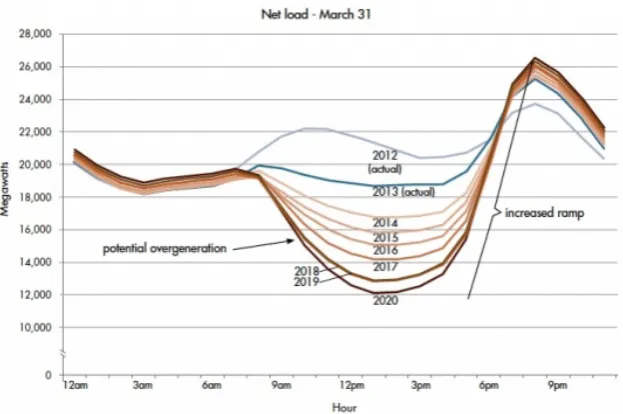
• Solar and wind are variable non-dispatchable energy sources, which means that they do not have a constant output of power and the amount of energy they supply cannot be increased or decreased like fossil fuel or hydro plants can. With the increase of solar and wind power on both local and national level, an increasing amount of generated energy is now ’uncontrollable’. This means that it is more difficult to match the supply to the demand, as all demanded energy has to be supplied at the exact moment the demand occurs. The problem is clearly visible in the duck curve, shown in Figure 1 [1]. In this figure, the net load represents the difference between the energy demand and the renewable energy production by solar energy. This is exactly the amount of energy that has to be generated with sources other than solar power. Therefore, the amount of fossil fuels needed may be reduced during the middle of the day (between noon and 4 p.m.), but the peak demand at around 8 p.m. does not decrease. As the power generation of big conventional power plants is not very flexible, for example because of long start up times, it may not be possible for them to increase their production as fast as the ramp indicated in the figure. This means that even during the middle of the day the conventional power plants are running at almost full capacity to meet the peak demand in the evening. Therefore, the need for fossil fuel plants stays, which may be a problem economically as now the introduction of renewables do not reduce the cost of energy from conventional power plants. Furthermore, during the middle of the day there is even a chance of overproduction of energy. As can be seen in the figure, this problem is expected to only increase in the future.

(7)

[image:7.595.147.459.108.315.2]

Figure 1: ’Duck curve’, showing the actual and future daily fluctuations of power that has to be generated with conventional power plants.

introduction of electric vehicles and electric heating, an increasing amount of electricity is needed to fulfill the demand that was previously met by petrol and natural gas. A higher demand of energy results in higher stress for the grid, which again is especially problematic for the distribution grid. A too high demand can lead to the same problems as the ones described in the first bullet, overloading and over- and under-voltage.

Basically, the above three problems all come down to an increasing mismatch between demand and supply of energy. This mismatch is faced on a national level, but equally (and maybe even more) important, on the distribution grid level. On both levels it leads to undesirable environmental results, as renewable energy might be discarded in times of overproduction. This is mainly the responsibility of policy makers. However, on the distribution grid level, it can also lead to grid malfunctioning, of which the DSO is responsible.

1.2 Solutions from literature

Much research is done to suggest solutions for the problems mentioned in the previous section, see e.g. [2] for an excellent review article about optimal operation and [3] for a review article about active management. The mentioned solutions can be divided into two categories:

1. Solutions that reduce the stress on the distribution grid,

2. Solutions that reduce the gap between demand and supply.

An overview of suggested solutions is given below, followed by a (1) and/or (2) to indicate the cat-egory of the solution. Note that reducing the gap between demand and supply at the distribution level automatically results in reducing the stress on the distribution grid.

(8)

• Network configuration changes. By changing switches and therefore the grid topology, the power can be send via different routes to resolve stress on certain parts of the grid. For (nearly) critical situations in the distribution grid, the local grid can also be switched to islanded mode, meaning that it is disconnected from other parts of the grid as to not influence the rest of the network. Changing the network configuration might also be used for phase balancing for multi-phase networks. The deployability of this method however depends on the grid topology, as there should be space to install switches and extra connecting lines. (1)

• Coordinated voltage control. The voltage profile within the distribution grid can be regulated by using controllable devices like on-load tap changers, decreasing the chance of facing over-or under-voltage. (1)

• Reactive power compensation and adaptive power factor control. Reactive power should be balanced as well as active power, and this can be done both by taking or injecting reactive power into the grid and by using the reactive power from distributed generation. It has to be noted that as in the distribution network the R/X ratios are generally quite high (i.e. the resistance is a lot higher than the reactance), using the reactive power generally has a low impact. (1)

• Curtailing renewable energy sources. This means that part of the electricity generated by wind and solar is not allowed to be injected in the grid, implying that it is wasted, in order to lower supply. This can be done either for state or corporate owned solar or wind farms (1) and for domestic generation. (1) & (2) However, as mentioned before, this option reduces the amount of electricity generated from renewable energy sources, while it was the initial goal to increase their share. Therefore, curtailing renewable energy sources is undesirable and the use of it should be minimized. To enforce this, some governments already have set a maximum for the amount of domestic generation that can be curtailed, also in order not to discourage civilians to install distributed generation. A DSO should have good agreements with its customers about when curtailment is allowed, and using it in order to resolve stress in the local network should be done in a fair way, such that all households are treated equally. This is discussed in more detail in Section 2.4.

• Curtailment of demand. This means that part of the energy demanded by the customers is denied by the DSO, in order to lower the demand. This option is undesirable and the use of it should be minimized because it can effect customer comfort quiet severely. Therefore good arrangements should be made with the customers about how often it is allowed and what form of compensation is possible. (1) & (2)

(9)

network. The flexibility of these appliances is however limited, and it is expected that they are only partially able to solve the problems. Furthermore, changing the behavior of appliances can lead to a decrease in comfort, depending on the customer, the appliance and the situation. Therefore, customers willing to shift their flexible appliances should be compensated by giving them monetary or social incentives. See [4], [5] and [6] for detailed descriptions of how flexible devices can be used for both grid stability and reducing peaks.

• Batteries. A battery stores energy to use it at a later moment, meaning that it shifts energy over time. It can be used to reduce the gap between supply and demand, as it can be charged at times of high supply and discharged in times of low supply. Ideally, this could totally match supply and demand and therefore solve all the aforementioned problems. However, a very large amount of batteries would be needed for this, and at quite a high price. Furthermore, batteries do not have an efficiency of a hundred percent, which means that energy is lost while shifted over time. Next to this, a battery has a finite life time, as it loses capacity with each charge/discharge cycle. Batteries can both be used to (partially) mitigate the variability of big wind or solar farms (1) and on a domestic scale to aid smart management of a household (1) & (2). The reader is referred to [6], [7] and [8] for ideas for optimal charging/discharging strategies.

• Electric vehicles. An electric vehicle can be seen as part of the problem, as it increases the total demand of energy. However, it can also be seen as part of the solution, as an electric vehicle is a very flexible appliance. If the charging time of an electric car is smaller than the time it is connected to the grid until it is needed again, the vehicle can be charged in times of highest supply. An electric vehicle can even be seen as a supplementary battery, as energy stored in the vehicle can be used to fulfill demand of a household or even be injected into the grid in times of low supply. This principle is known as vehicle to grid (V2G) and is an upcoming strategy to maintain grid balance, see [9] for a good example of how this flexibility can be used. (1) & (2)

1.3 Research question and organization of the thesis

It is probable that all solutions listed in the previous section are of importance and should be combined to face the problems caused by the energy transition, as they all have their strengths and weaknesses. This research however focuses only on the solutions that both reduce the stress on the distribution grid and reduce the gap between supply and demand, i.e. the solutions characterized by (1) & (2). These are: curtailing renewable energy sources, curtailment of demand, flexible appliances, batteries and electric vehicles. To the best knowledge of the author, no research has yet been done that uses this combination of solutions for trying to reduce the gap between demand and supply on both the national and the local level.

Note that all the mentioned solutions are taking place within the residential distribution network. The two stakeholders involved in these solutions are:

• The DSO: The distribution system operator has the power to forcefully lower demand or supply, as he can curtail the residents both if they are demanding too much energy from the grid or if they are injecting too much energy into the grid.

• The residentials: The residentials can use the flexibility of their flexible appliances, batteries and electrical vehicles, to either increase or decrease their net power (which is defined as their supply subtracted from their demand).

(10)

and management systems are needed to use the flexibility of the residentials in the right way. This is the core of this research, leading to the following main research question:

How can residential energy prosumers be motivated to use their flexibility to reduce the gap between supply and demand, while at the same time increasing distribution grid stability?

(11)

2 Distribution grid topology

In this section the distribution grid topology is discussed. With the knowledge of this grid struc-ture, the problems that can occur in the LV-grid are addressed and it is examined how residential energy users can help solving these problems. Furthermore, it is discussed how a distribution system operator (DSO) can ensure grid stability by forcefully changing the demand or supply of the prosumers, and how this can be done in a fair way.

2.1 Formal definition of the grid topology

For this research, a single-phase low voltage distribution grid with multiple households is consid-ered that is connected to the medium voltage grid with a transformer. The voltage level at the transformer can vary slightly due to fluctuations in the medium voltage grid, but it is assumed that this level is not affected by changes in the distribution grid. The transformer is supplying the households with energy and is also able to transport injected energy by the households to the medium voltage grid and it is assumed that the transformer is not limited in its capacity, meaning that it can handle infinite supply and demand. However, at the household level we take into account restrictions on the supply and demand because of limited grid capacity. The topology of the grid analyzed in this research can be characterized as radial in contrast to a mashed structure, i.e. the households are connected with lines in a branch-like structure, so there are no cycles in the network. Bidirectional power flow is possible and the lines can have different specifications for type and thickness, resulting in varying line resistance and maximum power flow. All households produce a time-dependent net power curve over the day, which represents their energy demand minus their supply at a certain time. As prosumers are assumed to be able to both supply to and demand from the grid, the net power can be either positive in times of higher demand, negative in times of higher supply or zero in times of equal demand and supply. The voltage level at each household is varying, dependent on the power flows and the properties of the cables.

More formally, the distribution grid is defined as a directed rooted tree RT = (V, E), where all edges are pointed away from the root, known as an out-tree. Here,V ={vT R} ∪VH∪VCis the set of vertices, wherevT Ris the transformer and the root of the tree,VH is the set of households and

VC the set of connection points where multiple lines come together. As we are interested in the evolving of the grid over time, we also have to model the time. We do this by discretizing the given time horizon in a setT of time steps. To specify the net power injected or withdrawn from the grid at a nodev ∈V at timet∈T, a variableN Pv(t) is attached to vertex v. As connection points

v∈VCdo not supply or demand energy, we haveN Pv(t) = 0 for these vertices. For all households

v ∈ VH, a total power injection at timet is represented with N Pv(t) <0 and a power demand is denoted with N Pv(t)>0. As the transformer is the root of the tree and should consume or supply the energy of all other nodes, it follows thatP

v∈VHN Pv(t) =−N PvT(t). Furthermore, to

(12)

2.2 Load flow analysis

Now that we have a formal definition of the grid topology, we can make a load flow analysis. With this analysis, we can find the power flowP Fe(t) and currentCe(t) over the edges and the voltage level V Lv(t) of the vertices, given the topology of the grid, the resistance Re of the lines and the net powerN Pv(t) of the households. The load flow analysis for meshed networks or 3-phase distribution grid is quite complicated, and special power system simulation software can be used for this analysis. However, for a single-phase radial network as considered in this research, the load flow analysis is rather simple. It is known as a forward/backward sweep algorithm [10], and is shown in the following subsections. First, the power flow is analyzed, which is needed to find the voltage level at each household. With the knowledge of the voltage, the current over all lines can be calculated. It is important to know both the currents of all lines and the voltage level at each household, as the grid-related issues discussed in this research (overloading and over- or under-voltage) are direct consequences of these values.

2.2.1 Power flow

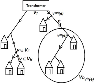
If power losses due to line resistance are neglected, the power flowP Fe(t) over an edge can be found by summing over the net powerN Pv(t) of all households that are descendants from this line (all the vertices further away from the root). IfVD_vin₍_e₎is defined as the set of all vertices in the subtree with vin₍_e_{) as root including vertex} _vin₍_e_{) itself, it follows that} _{P F}

e(t) =Pv∈VD_vin₍_e₎N Pv(t) is

[image:12.595.149.455.436.706.2]

the flow in edge e = (vout(e), vin(e)). A negative power flow is a flow in the direction towards the root and a positive power flow is a flow away from the root. See Figure 2 for a graphical representation of a LV distribution network and the setVD_vin₍_e₎.

(13)

2.2.2 Voltage level

The voltage level V Lv(t) is varying across the grid, because sending power over an edge e = (vout₍_e₎_{, v}in₍_e_{)) requires a difference in voltage between the two vertices. The exact amount of} voltage difference is dependent on the resistance and the reactance of the lines, as well as both the active and reactive power flow. However, as for low voltage networks the reactance of lines is relatively small compared to their resistance, the reactive power is often neglected and therefore the following simplification for the voltage difference is made:

V Lvout_(e)(t)−V L_vin_(e)(t) =

Re·P Fe(t)

V Lvin_(e)(t)

. (1)

As we assume that the voltage of the transformerV LvTR is known, the voltage levels of the other

vertices can be found iteratively, starting from the transformer down the entire tree. Rearranging (1) results in

(V Lvin_(e)(t))2−V L_vin_(e)(t)·V L_vout_(e)(t) +Re·P Fe(t) = 0. (2)

The value forV Lvin_(e)(t) can be found by solving the quadratic equation (2). This results in two

values, where the smallest solution represents the voltage drop, and the largest solution is the desired voltage level at the incoming vertex.

2.2.3 Current

The currentCe(t) can then easily be found by using Ohm’s law, which states that

Ce(t) = V Lvout(t)−V Lvin(t)

Re(t) . (3)

2.3 Potential grid problems

In this section two potential grid problems are described. As this research focuses on mitigating these problems by using the flexibility of consumers, it is also discussed which households have influence on these problems. Then, possible solutions to the problems are proposed.

2.3.1 Overloading

A problem occurs when too much current is send over a line, resulting in too much heat generation within some components of the electricity circuit. Every type of line has a specific value for the maximum amount of current that is allowed to flow through it. This means that for every edge

e= (vout₍_e₎_{, v}in₍_e_{)) and all times}_t_∈_T_{, we should have}_|_C_e(_t₎_{| ≤}_CCC_{e, where}_CCC

erepresents the current carrying capacity for edgee. We speak of overloading if the current becomes higher than the current carrying capacity.

(14)

the power flow. Therefore, the only households that are able to mitigate this problem, are those householdsv∈VD_vin₍_e₎, see Figure 2.

The problem of an overloading of the edgee= (vout₍_e₎_{, v}in₍_e_{)) can be solved by adjusting (either} voluntarily or forced) the total net powerN Pv(t) of the householdsv∈VD_vin₍_e₎. Because the net power is proportional to the current, the total net power should be reduced with the same factor as the current is outside its flow limit. If α=|Ce(t)|/CCCe represents the factor of how much the current carrying capacity is exceeded, then the needed total net power N T N PVD_vin₍_e₎(t) is

calculated as

N T N PVD_vin₍_e₎(t) =

P

v∈VD vin(e)

N Pv(t)

α . (4)

The households v ∈ VD_vin₍_e₎ should therefore change their net power to values N Pvnew(t), such that

X

v∈VD vin(e)

N P_vnew(t) =N T N PVD_vin₍_e₎(t). (5)

2.3.2 Under- and over-voltage

The voltage level V Lv(t) at each household v ∈ VH and time t ∈ T should stay in between a minimum and maximum voltage level V L− and V L+_{, because too high or too low voltage is} harmful for electrical components. Voltage regulation is therefore very important and can be done in multiple ways, as discussed in Section 1.2. In this report however, the focus is on keeping the voltage level within bounds by using the flexibility of customers. This can be achieved because, looking back at Section 2.2.2, the voltage drop between two households depends on the amount of power that is sent over the line between them. Basically, a higher net power (by increasing demand or reducing injection) decreases the voltage and a lower net power (by decreasing demand or increasing injection) results in a voltage increase.

If a household changes its net power, a different amount of power is send over all the lines leading from the transformer to that household. Because the voltage drop depends on the power send over a line, the voltage level changes at all households on that path. Furthermore, all descendants (i.e. vertices further away from the root) of those households also get a different voltage level, because the voltage level at a vertex depends on its ancestor vertices. Therefore, in case of an under- or over-voltage at a certain household, all household that are descendants from the edge from the transformer to the highest ancestor of the household with a problem e= (vT R, vin(e)) are responsible for and able to help solving the under- or over-voltage problem. In Figure 3 this situation is sketched, where VD_{V in}₍_e₎ is the associated set of households. Note, that if only one branch is going out from the transformer, all households in the grid are responsible for and able to help solving an under- or over-voltage problem.

(15)

Figure 3: Graphical representation of a LV distribution network with an under- or over-voltage problem at the bolt icon.

SMij =

     

∂V L1(t)

∂N P1(t)

∂V L1(t)

∂N P2(t) . . .

∂V L2(t)

∂N P1(t)

∂V L2(t)

∂N P2(t) . . .

.. . ... . ..       (6)

Note that if there is only 1 outgoing edge from the transformer, all entries of the sensitivity matrix are strictly bigger than zero, whereas in the case of multiple outgoing edges from the transformer, households in different branches (with the transformer as root) will have a sensitivity of zero. Using this sensitivity matrix, we assume that the change of net power in householdiis proportional to the change in the voltage level for household j for alliandj. To check whether this assumption is reasonable, first we look at Ohm’s law. According to this, the change in voltage of a household is proportional to the change in net power for the same household. To see why the voltage level in one household is also (approximately) proportional to the voltage level in other households, one has to look back at (2) in Section 2.2.2. Solving this equation leads to

V Lvin(e)(t) =

V Lvout_(e)(t) +p(−V L_vout_(e)(t))2−4·(R_e·P F_e(t))

2 . (7)

Above equation gives the direct relation between the voltage levels of two neighboring house-holds. To see why these voltage levels are approximately proportional, we look at the derivative

∂V L_vin₍_e₎(t)

∂V L_vout₍_e₎(t), which represents the change in the voltage level of the incoming vertex due to a change in voltage level in the outgoing vertex. For typical LV-grid values Re = 0.0738, P Fe(t) = 3000 andV Lvout(e)(t) = 230, the derivative of (7) toV Lvout(e)(t) is 1.00424. A value of 1 would mean

a perfect proportional relation, so we see that using the sensitivity matrix gives us a rather good approximation for the change in voltage levels.

(16)

change. With the sensitivity matrix, it is now rather simple to calculate the amount of net power that the households should shift if an under- or over-voltage problem occurs. LetV Vv(t) represent the voltage violation at householdv and timet. It can be defined as

V Vv(t) =

  

 

V Lv(t)−V L+ _if_{V L}_v(_t₎_{> V L}+

0 ifV L−≤V Lv(t)≤V L+

V Lv(t)−V L− ifV Lv(t)< V L−.

(8)

Now the goal is to solve the voltage violations by changing the net powersN Pv(t) for households

vat timet. As can be seen from (8), the voltage violationV Vv(t) at householdv at timetis zero when the voltage levelV Lv(t) is within bounds. Therefore, a corrective action from the households is needed such that the voltage level increases (for under-voltage) or decreases (for over-voltage) at least withV Vv(t). The size of the corrective action for an under- or over-voltage problem at household i, that we define asN Pchange

v (t), can easily be calculated with the sensitivity matrix defined in (6):

X

v∈VH

N P_vchange(t)·SM_i,T_∗=V Vi(t), (9)

whereSMi,∗ represents the ith row of the sensitivity matrix. Similar to the overloading scenario

described in Section 2.3.1, the households should therefore change their net power to desired values

N Pnew

v , where these new net powers are defined as

N P_vnew(t) =N Pv(t) +N P_vchange(t). (10)

2.3.3 Phase imbalance

In this research a single-phase network is analyzed for reasons of simplicity. However, using the flexibility of energy prosumers is expected to be able to mitigate another potential problem that occurs in a 3-phase network as well. In a 3-phase network it is important that the total loads on the three different phases have similar values. Therefore, it should hold thatP

vN P1v(t)≈

P

vN P2v(t)≈

P

vN P3v(t), whereN P jv(t) represents the net power on thej

th_{phase. Using the}

flexibility of the households, the load on the three phases can be changed towards for example the average of them. This idea is out of the scope of this report, but can be used for future research.

2.4 Incentives, curtailment and fairness

In the previous sections it was seen that local grid problems can be (partially) solved by the flexi-bility of the energy prosumers in that network. However, it is the responsiflexi-bility of the distribution system operator (DSO) to maintain grid stability, and not that of the households. Therefore, the energy prosumers should be motivated by the DSO to actually use their flexibility and adjust their net power in the direction needed by the DSO. In Section 3, possible incentive structures offered by the DSO are discussed in more detail.

(17)

solve these issues without the flexibility of prosumers, like spinning reserve in case of too much demand or batteries in case of too much injection. In this research however, it is assumed that the DSO does not have access to these options and should solve the problem with the flexibility of the prosumers only. This means that in extreme cases the DSO can force households to increase or decrease their net power, by not allowing respectively part of their injection into the grid or part of their demand from the grid. In this report, they are named respectively injection curtailment and demand curtailment (note that demand curtailment is not a common term, but is used here because of the similarity with injection curtailment). In reality, it depends on regulations and agreements between the DSO and the prosumers whether injection and/or demand curtailment are allowed [11] [12].

Assuming that DSO’s can forcefully change the net power of the households in the grid, a grid-related issue can be completely solved by curtailing (some of) the prosumers. However, it is not clear from previous sections which of them should be curtailed. The solutions proposed in (5) and (9) to solve the grid-related issues state a vector of new desired net powerN Pnew

v (t), which is a joint solution of all households that have influence on the grid related issues, i.e. v ∈ VD_vin₍_e₎. This vector of new desired net powers is however not unique, as different combinations of curtailed households can solve the grid-related issue.

The problem is therefore that there are many possible actions that reach our goal of solving grid related issues, but it is not clear which one to choose. For example, assume that an over-voltage problem occurs at householdiand both householdsiandj are able to solve it. Should household

isolve it, because the issue is located at his household? Or should the household with the lowest net power (the biggest contributor to the over-voltage problem) solve it, or should they solve it together in a certain ratio? There is no best solution for this problem, but there are some ideas in literature about how to divide curtailments in a ’fair’ way. Fairness is a very subjective term, but it basically comes down to treating all households (as much as possible) in the same way, and not curtailing one household more because of e.g. its physical location in the grid. Some options include [13]:

• All households that have influence on the problem should change their net power with the same amount. In this option everybody is curtailed equally.

• All households that have influence on the problem should change their net power with the same percentage. In this option prosumers that have a higher absolute net power are curtailed more than prosumers with a lower absolute net power, which means that bigger contributors to the problem should also help more.

• Households with a greater influence, i.e. higher value in the sensitivity matrix for under- or over-voltage, should change their net power more than households with a lower influence. This option is less fair, as now the physical location in the distribution grid is taken into account for the amount a household is curtailed. However, with this option a lower total amount of curtailment is often needed, as higher values in the sensitivity matrix result in a bigger voltage change per net power change for under- and over-voltage problems.

• A maximum (for demand curtailing) or minimum level (for injection curtailing) for the net power is set for all households that have influence and values below or above these bounds are curtailed up to this bound. In this option only the highest contributors of the problem are curtailed.

(18)

(19)

3 Incentive structure for residential energy users

In this section it is discussed by which means residential energy users can be motivated to use their flexibility. First it is discussed which types of incentives are available, then it is analyzed what the requirements are for an incentive structure that is suitable for the problem formulated in this research and lastly a novel price/incentive structure is proposed.

3.1 Possible incentives

To motivate consumers to offer their flexibility to the grid, they should be offered some form of reward. A consumer might have made an investment by buying a battery, or his comfort may decrease because of a change in the operation of his appliances. To compensate him/her for this, an incentive is needed that results in the desired behavior of consumers. Incentive structures that are offered in the field can be divided into three categories [14]:

• Social incentives. Ideas are emerging to gamify demand response, which means that elements from game playing are applied to intrinsically motivate people. For example, households can all be connected to a sort of scoring board, to rate them based on their sustainable performance. It is expected that in many cases intrinsic motivation is not enough to persuade people, especially when a monetary investment has to be earned back, but it can be combined with monetary incentives for extra motivation.

• Price based incentives. By offering different energy prices during different times of the day, people are motivated to shift their energy consumption to cheaper time periods and their injection to more expensive periods. This can range from a Time of Use (ToU) program, in which generally two or three pre-set price levels are offered, to a Real Time Pricing (RTP) program, in which the price can fluctuate real-time over the whole time period, following in general the market price of electricity.

• Event based incentives. In this option an event that lasts for a certain time is announced to which people can react. This can be a monetary reward for increasing or decreasing normal energy consumption within the event, a bonus for self-consumption within the event, a penalty for injection within the event, a periodic reward for offering a certain amount of flexibility, etc.

3.2 Requirements for an incentive structure

(20)

has the highest priority. Therefore, the DR-signals based on the national situation offered by the utility or an aggregator should be able to be changed or overruled in case of a local distribution grid problem, so that customers are motivated to help mitigating these local issues first.

3.3 Multi-level real time pricing with traffic light

The basic idea for a novel price/incentive structure for residential energy users that fulfills the requirements of the previous section is a price based DR-program that is dependent on both the national situation and on the situation in the local distribution network. A multi-level real time pricing (RTP) is proposed, in which the energy price can change minutely, quarterly or hourly, but can only switch between a fixed amount of price levels. For example, a 5-level RTP would look as follows:

• ++ lowest price (per kWh), extreme amount of generation, possible injection curtailment.

• + low price (per kWh), larger need for demand than for supply.

• 0 average price (per kWh), normal situation.

• −high price (per kWh), larger need for supply than for demand.

• −− highest price (per kWh), extreme amount of demand, possible demand curtailment. For every time frame the utility offers one of these prices to its customers, based on e.g. the prices at the national energy markets. However, this price can be adjusted or overruled if an issue arises within the local grid, because local issues should be solved first. This is done by assigning a traffic light to each household that can change with time, reflecting the local grid situation at that particular household at that time. The three colors of the traffic light imply the following:

• Green: No problems in the grid (that the household can help solving); apply the price offered by the utility.

• Orange: Risk of problems (that the household can help solving); dependent on the type of problem, the price level offered by the utility is adjusted one level up (in case of desired lower net power) or down (in case of desired higher net power).

• Red: Extreme problem (that the household can help solving); dependent on the type of problem, move to level −−or ++, curtailment necessary.

A red light is given in situations where the limits for the voltage levelV L−andV L+_{or the current} carrying capacityCCCe are really exceeded, so that curtailment is necessary. The orange traffic light is a warning signal and can be set at for example 80% of the limits to encourage households to change their loads before they have the risk to be curtailed.

To clarify the traffic light mechanism, an example is given here. If there is a risk of under-voltage in one of the households, all households that have influence on its voltage level will get an orange light. If the utility is offering price level +, these houses are now offered level 0, so that with this higher price they are stimulated to demand less or supply more, increasing thereby the voltage level. If this is not enough and the voltage level decreases to a problematic value, these houses will get a red light and are offered−−, to stimulate them with even higher prices to further increase the voltage. If offering high prices does not suffice in decreasing demand or increasing supply, the DSO will curtail the prosumers with the highest demand.

(21)

(22)

4 Household optimization

In this section, first the situation for the households is sketched, followed by an optimization program that is derived for the flexible devices. As it might be too time-consuming to solve this optimization, heuristics are designed that find sub-optimal management decisions for the flexible devices.

4.1 Situation

In the previous section a new pricing scheme was suggested in which the price of energy that prosumers pay for demand and receive for injection could change every time step, e.g. minutely. In this scheme, the prosumers are motivated by these different prices to lower their demand or increase their injection (e.g. by discharging their battery) in times of high prices, and increase their demand or decrease their injection in times of low prices. However, it is not clear how exactly they should use the flexibility of their devices to respond to these changing prices in an optimal way. An optimal strategy is difficult to find, as the decisions depend on for example the current and future energy prices, the current and future generation, the situation in the local grid and therefore the chance of curtailment, the state and parameters of all flexible devices, the demand of the non-flexible devices, their comfort preferences, etc.

As the price might change minutely in this pricing scheme, it is assumed that all decisions are made automatically, as it is extremely impractical for humans to change the behavior of their appliances constantly. Therefore, it is assumed that within a household a very advanced communication system exist that connects all devices with an automatic managing entity, and that this entity can control all these devices. Furthermore, it is assumed that it is possible for DSO’s to curtail an exact amount of both demand and injection. Next to this, the assumption is made that a good prediction of both the energy prices and the generation is available for the managing entity. The decisions that the management entity makes for the flexible devices is discussed in the following subsections.

4.2 Optimization for the flexible devices

The flexible devices are divided into four different groups [15]: shiftable appliances, thermal appli-ances, batteries and electric vehicles. They are all managed so that the energy costs are minimized, based on the current and predicted energy prices, using discretized time steps. In the following four subsections, the optimization is derived for the four groups of flexible devices individually, followed by a combined optimization program.

4.2.1 Shiftable loads

Shiftable loads are loads that can be shifted in time (i.e. they can be run later or earlier), like dish washers or clothes dryers. Let A be the set of all shiftable loads. The flexibility of such a loada∈A is its starting timeSTa. A consumer can restrict times for the use of the appliance to limit his comfort reduction, by defining an earliest starting timeESTa and a latest finishing time

LF Ta. If the running time of an appliancea∈Ais denoted byRTa, the set of (discrete) possible starting timesP STa can be described as:

(23)

Let the energy profile of a shiftable appliance a∈ A be denoted by (SAPa,1, ..., SAPa,RTa). As

mentioned before, it is assumed that the energy priceEPtis known or a prediction can be made for all future timest∈T. To minimize the energy cost, a start timeSTa should be found so that the appliance runs in the cheapest times. Mathematically, this means that we minimize

min STa∈P STa

STa+RTa

X

t=STa

EPt·SAPa,t−STa+1. (12)

4.2.2 Thermal loads

Thermal loads are loads that control the temperature in a certain space, like an air conditioner or a deep freezer. LetB be the set of all thermal loads. Usually, a thermal loadb∈B is used to keep the temperatureT EM Pb,t in a space at timet∈T close to a set point temperatureSP Tb. It is assumed that the temperature always has to be within a deadband temperatureDBTb and this constraint is mathematically defines as

SP Tb− 1

2DBTb≤T EM Pb,t≤SP Tb+ 1

2DBTb ∀b∈B,∀t∈T. (13) Thermal appliances can be either on or off. This is represented by a binary variableT ASb,t which expresses the thermal appliance state of appliance b at time t ∈ T (1 for on, 0 for off). It is assumed that the change in temperature is independent of the outside temperature, and that the thermal appliance is used to cool a space (the optimization is similar for a heating device). This implies that there is a cooling parameterCPb that depicts the amount of temperature change in one time step when the appliance is on, and a heating parameterHPb for the temperature change in one time step if the appliances is off. IfT EM P0represents the temperature at the start of the time horizon, the course of the temperature is then described by

T EM Pb,t+1=T EM Pb,t+T ASb, t·CPb+ (1−T ASb,t)·HPb ∀b∈B,∀t∈T. (14)

Let the electricity consumption of thermal loadb∈B be denoted byT ACb. This implies that the electricity demandT ADb,t at timet of the thermal appliance is given by

T ADb,t=T ACb·T ASb,t ∀b∈B,∀t∈T. (15)

To minimize the energy cost, the thermal appliance should be scheduled such that it produces demand in the cheapest time steps. This results in the following optimization problem

minX t

EPt·T ADb,t ∀b∈B, (16)

under the constraints of (13), (14) and (15). It should be noted that this optimization will always result in the highest temperature SP Tb+ 1₂DBTb at the last time frame t = |T|. To prevent this, the objective function can be adjusted so that a lower temperature at the last time frame is rewarded accordingly, this leads to the following objective;

minX t

EPt·T ADb,t+

T EM Pb,|T|−(SP Tb−1₂DBTb)

CPb

(24)

4.2.3 Battery

A battery is a device that can store energy by charging it at one time and discharging it at another time. The battery’s state of chargeBSCt at timet∈T is chosen as a variable between 0 and 1 that reflects the relative state of charge, i.e. it is found by dividing the battery’s current stored energy BSEt by the maximum possible amount of stored energy BSE+. A customer can set a minimum and maximum state of charge BSC− and BSC+ _{other than 0 and 1 according to his} preferences, implying the constraints

BSC−≤BSCt≤BSC+ ∀t∈T. (18)

The amount of energy that a battery charges or discharges in time steptis denoted by a variable

BCDt, which is positive for charging and negative for discharging. It is assumed that a battery can charge and discharge at all levels between the maximum charge and discharge speeds M BC

andM BD, i.e. we have

M BD≤BCDt≤M BC ∀t∈T. (19)

Let the state of charge of the battery at the beginning of the planning horizon be denoted by

BSC0. Then the course of the battery’s state of charge is described by

BSCt+1=BSCt+

BCDt

BSE+ ∀t∈T. (20)

Unfortunately, due to technical constraints, some of the energy is lost when it is first charged and later discharged, meaning that the efficiencyBE of a battery is not 100%. To model this, a variableαtis introduced that is defined as

αt=

(

1 ifBCDt≤0

BE ifBCDt>0.

(21)

This implies that we consider the inefficiency of the battery only when charging. The optimal charging and discharging of the battery looking at future prices can now be solved by finding

maxX t

EPt·αt·BCDt, (22)

under the constraints (18), (19), (20) and (21). As with the thermal loads, the above optimization always results in an empty battery at the end of the time period, and therefore the following ad-justment can be made to reward a higher state of charge at the end of the time period accordingly:

max BCDt

X

t

(25)

4.2.4 Electric vehicle

An electric vehicle can be seen as a flexible demand, as the energy it requires for driving can be supplied at variable times, as long as it is charged in time. On the other hand, when the vehicle is idle and connected to the LV distribution grid, it can be seen as a battery as well. This means that not only energy may be taken from the grid for storage, but also energy stored in the electric vehicle may be injected back into the grid. This concept is known as ’vehicle to grid’ (V2G). Based on the above, the electric vehicle is modeled like the battery, only with some extra constraints. Instead of a constant minimum state of charge for the battery, the consumer can set a variable minimum state of charge for the electric vehicle V SC_t−, so he/she can ensure for example that his/her car is fully charged in the morning, or that he always has a certain amount of energy in case of an emergency. This is modeled as

V SC_t−≤V SCt≤V SC+ ∀t∈T, (24)

whereV SCtdenotes the state of charge of the electric vehicle at timet∈T. The amount a vehicle can charge and dischargeV CDtis, similar to the battery, limited byM V C andM V D;

M V D≤V CDt≤M V C ∀t∈T. (25)

For an electric vehicle, it should furthermore be known in which time steps it is connected to the grid. When it is not connected, the vehicle cannot be used as a flexible device and it is consuming energy for transportation. Whether or not the vehicle is connected to the grid is depicted with a binary parameterV Gt.

The amount of energy that an electric vehicle consumes for transport is very dependent on the user of the vehicle, e.g. how far his/her work is and whether a charger is available there. Research can be done to analyze the driving behavior of owners of electric vehicles and even machine learning strategies can be used to make more precise predictions. However, this is not part of this research and therefore a simplification is made. It is assumed that the energy consumed is proportional to the time that the car is not connected. This implies that for every time steptthat the vehicle is not connected to the grid, it consumes a constant amount of energyV EC. A variable V CD∗_t is introduced to model this, and is defined as

V CD∗t =

(

V CDt ifV Gt= 1

V EC ifV Gt= 0.

(26)

Let the state of charge of the vehicle at the beginning of the planning horizon be denoted with

V SC0. The course of the vehicle’s state of charge is then described by

V SCt+1=V SCt+

V CD∗_t

V SE+ ∀t∈T. (27) Like a normal battery, the battery of the electric vehicle also does not have an efficiency V E of 100%, therefore a variableβtis introduced that is defined as

βt=

(

1 ifV CD∗

t ≤0

(26)

Similar to the normal battery, this implies that we consider the inefficiency only while charging. Now, the optimal strategy for the electric vehicle can be found by solving

max V CD∗

t

X

t

EPt·βt·V Gt·V CDt∗+V SE|T|·EP|T|, (29)

under the constraints of (24) - (28). The termV SE|T|·EP|T|was added in (29) to reward a higher

state of charge of the vehicle at the end of the planning period accordingly. Furthermore, note that the termV Gtis added so that energy is only paid for in times the vehicle is connected.

4.3 Joint optimization

The four optimization problems described in the previous subsections can now be combined. To this combined model we add the own generation of a household. For this, let Gt represent the current or predicted own generation at time stept. Furthermore, for a shiftable devicea∈A, let

SAIa,tbe an integer variable that only takes value 1 ift∈P STa, i.e. if the time step is a possible starting time for device a. If we now define the net powerN Ptof a household as the amount the household is demanding (N Pt>0) or injecting (N P <0) at timet, we get

N Pt=

X

a∈A

SAIa,t·SAPa,t−STa+1+

X

b∈B

T ADb,t−αt·BCDt−βt·V CD∗t−Gt ∀t∈T. (30)

Then the function that should be minimized is given by

X

t∈T

EPt·N Pt, (31)

which has decision variables STa, T ASb,t, BCDt and V CD∗t. This objection function is just the combination of the objective function of the four different kind of flexible units described in (12), (17), (23) and (29), however without the extra objective for preventing minimal energy storage at the last time step. This objective function should be minimized under the constraints for the four types of flexible units described in the previous subsections.

Within the pricing scheme with traffic light described in Section 3.3, the energy price EPt is dependent on the net powers of all households at timet, because for high values ofN Ptthe traffic light can result in different prices and curtailment. Note, that curtailment can also be seen as a change in energy price, where injection curtailment corresponds with a price of EPt = 0 and demand curtailment with an extremely high price. Therefore, the objective function (31) is not a linear function. Only if we assume that a prediction of the prices (including curtailment) can be made, the objective function is almost linear. Almost, as looking at the first part of (30) we see that the objective function for the shiftable devices is not linear, as the decision variable STa is used within the index of the variableSAPa,t. However, there are standard techniques available to also change this part into a linear program, by making the start time a time-dependent vector and setting P

tSTa(t) = 1∀a ∈A. (This is not further worked out here, and the reader is referred to [16] for more details.) As the objective function can be made linear, all constraints are linear and some variables and artificial variables needed for the constraints are integers, the described optimization problem can be identified as a mixed integer linear program (MILP).

(27)

amount of variables. If time steps are chosen as minutes and an optimization is to be made for a whole day, we need to model 1440 time steps, resulting in a very large amount of variables. Furthermore, as the prediction for the energy price and own generation and consumption can change quite often, it probably will not suffice to make one schedule for the whole horizon, so the optimization preferably runs every time new data is available. Lastly, the assumption that the energy price EPt (including changes due to the traffic light) can be predicted is a little unreasonable, as the traffic light depends on the behavior of all other prosumers in the grid and is therefore very difficult to predict. Dropping this assumption would only further complicate the optimizations.

Because of the above stated reasons, it is chosen not to try to optimize the behavior of the flexible devices, but to develop heuristics that are not so time consuming. These heuristics decide on the behavior of the devices at every time step, and should have a sufficiently good performance. The developed heuristics are discussed in the next subsection.

4.4 Heuristics for the flexible units

Because of the high calculation time needed to optimize the problem for a large amount of time steps and the assumption made about the predictability of future energy prices, it seems to be more suitable to find a heuristic that is executed every time step to determine the actions that should be taken for the current moment, and leads to a sufficiently good solution. This heuristic does not have to make a whole schedule for the flexible units like the optimization tried to do, but it only has to make a decision for the present time step, based on predicted prices, generation and consumption. The goal of the heuristics is to choose the decision variables for the present time for the four types of flexible devices as good as possible, i.e. the total energy bill should be as low as possible. The heuristics make decisions like in a rolling horizon method, where the decision for the current timeCT is based on the planning horizonCT, CT+ 1, ...CT+T, whereT is now the size of the planning horizon. In the following we describe such a heuristic approach, whereby we give for each of the four types of flexible devices a separate heuristic. Before giving these heuristics, we give in Subsection 4.4.1 some background on the role of self-consumption in these approaches.

4.4.1 Self-consumption

To prevent curtailment and changes of the prices as the result of traffic lights, it is beneficial for the prosumers to have a high self-consumption. This means that the energy they produce by for example solar panels, should be as much as possible consumed by themselves. A higher self-consumption reduces the stress on the local network, as it reduces both the total demand and total supply of a household. Therefore, the heuristic should take into account that it is better to consume energy in times of high own generation.

Within the 5-level pricing system, however, self-consumption is not always desired. For example, if the energy is expensive but is expected to become cheaper in the near future, a consumer that is generating energy at this moment can better sell his energy to the grid now, and consume energy at a later time when the energy is cheaper. This is both better for his energy bill and for the grid, as a high price indicates that more injection is needed and low prices indicate that more consumption is desired.

(28)

4.4.2 Shiftable appliances

Shiftable devices are assigned a set of possible starting timesP STa, defined as the time steps from the earliest starting timeESTa till the latest starting time LSTa. If the current time is within the set of possible starting times, i.e. ifCT ∈P STa, and the device has not started yet, the only decision to be made is whether the device should be started now (i.e. in the time frameCT), or later (i.e. in one of the time framesCT + 1, CT+ 2, ..., LSTa). Based on the current and future electricity pricesEPCT, EPCT+1, ...and the shiftable appliance profileSAPa,tit can be calculated how much it would cost to start now. Then, we iteratively compare the cost of starting now with the cost of starting in the next time stepsCT+ 1, CT+ 2, ..., up to the last possible starting time

LSTa. The comparison is stopped when a cheaper future start time is found, or when the costs are the same, but a higher own generation follows for the future time step (i.e. larger amount of self-consumption). In this case, the shiftable appliance will not start at the current time CT. If the iterative comparison does not find a better starting time thanCT, the current time is the best option and it is decided to switch on the shiftable appliance.

4.4.3 Thermal appliances

Thermal devices only have two possible states, they can be either on or off. Therefore, the only decision that has to be made is which of the two states should be chosen at the current time. The only constraint for thermal appliances is that it should keep the temperature within a certain deadband around the set point temperature. Based on the current temperature and the current and future energy price (and later also on the own generation), a heuristic is designed that tries to minimize costs within the temperature constraint. The heuristic is based on six principles:

• The thermal appliance should keep the temperature within bounds.

• The thermal appliance should be on in times of injection curtailment and off in times of demand curtailment.

• The thermal appliance should be on in cheap time steps and off in expensive time steps.

• The thermal appliance should not be on if an even cheaper time step is coming, and not be off if an even more expensive time step is coming.

• The thermal appliance should make sure that the room is cooled down to the minimum allowed temperature just before a more expensive time step is coming, and make sure that the room is heated up to the maximum allowed temperature just before a cheaper time step is coming.

• The thermal appliance should keep the room at the minimum allowed temperature in times of high prices (when there is a risk of demand curtailment) and at the maximum allowed temperature in times of low prices (when there is a risk of injection curtailment). This is done in order to have more response when demand or injection is curtailed. Note, that this seems to be in contradiction with the fifth principle. They can be combined, however, by keeping the temperature high in times of low prices, and only cool down just before the price is expected to increase, and vice versa.

(29)

the heuristic is to minimize the cost of the thermal appliance, and it basically does this by lowering the temperature to the minimum allowed temperature just before a more expensive energy price is coming, and increasing the temperature to the maximum allowed temperature just before a cheaper future energy price is coming up. More precisely, in the three cheapest price levels ++,+ and 0, the heuristic checks for how many time steps the price will not be higher than the current price. If there are enough of these time steps to bring the temperature from the current temperature to the minimum temperature, the heuristics decides not to cool down yet. Only if there are not enough of these time steps, the device will cool down so that just before the price increases, the temperature is at the minimum level. Similarly, in the two expensive price levels−− and−, the heuristic checks for how many time steps the price will not be lower than the current price. If there are enough of these time steps to bring the temperature from the current temperature to the maximum temperature, the heuristics decides not to heat up yet. Only if there are not enough of these time steps, the device will heat up so that just before the price decreases, the temperature is at the maximum level.

More formally, if the current temperature T EM PCT is too high, i.e. T EM PCT > SP Tb + 1

2DBTb, whereSP TbandDBTbrepresent respectively the set point temperature and the deadband temperature, the appliance has to cool down (i.e. be on). If the temperature is too low, i.e.

T EM PCT < SP Tb−1₂DBTb, the appliance should be off, resulting in a warmer temperature. If the temperature is within bounds, it is checked whether curtailment is applied. Two binary variables

ICB and DCB representing respectively the injection curtailment and demand curtailment are introduced, which take on value 1 if curtailment is applied, and value 0 if no curtailment is applied. If ICB = 1, the appliance switches on, if DCB = 1, the appliance switches off, and if ICB =

DCB = 0, the heuristic makes a decision based on the current temperature T EM PCT and the current and future energy pricesEPCT, EPCT+1, ...EPCT+T. For this decision, some new variables are introduced. LetT T Cbbe the number of time steps it takes to get from the current temperature

T EM PCT to the coldest allowed temperature SP Tb− 12DBTb while cooling. Furthermore, let

T T Hb represent the amount of time steps it takes to get from the current temperature to the hottest allowed temperature SP Tb+ 1₂DBTb while heating. Furthermore, let N CT(EPCT) be the number of future time steps within the planning horizonCT+ 1, CT + 2, ..., CT+T that are consecutively cheaper or equal to the present electricity priceEPCT and letN ET(EPCT) be the number of future time steps within the planning horizon that are consecutively more expensive or equal to the present electricity price. Then the heuristic makes the following decision:

• ifEPCT ∈ {++,+,0}:

state =

(

on ifT T Cb≥N CT(EPCT) off ifT T Cb< N CT(EPCT)

(32)

• ifEPCT ∈ {−−,−}:

state =

(

on ifT T Hb< N ET(EPCT) off ifT T Hb≥N ET(EPCT)

(33)

(30)

[image:30.595.86.533.259.476.2]

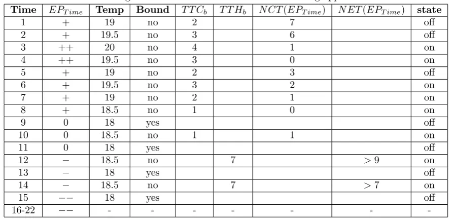
time step the temperature will be increased with half a degree. So even though the price is at a cheap level, the appliance does not switch on, because there are enough future time steps that are cheap (or even cheaper). In the second time step, exactly the same decisions is made. As only in time step 3 and 4 the price is at the cheapest level (++), in these time steps the appliance is on. At time step 6, the heuristic decides to cool down, as a more expensive period is coming up in time step 9, so it makes sure that at this time the temperature is at the lowest level, at 18 degrees. In time steps 11-14 the heuristic makes sure that the temperature is kept at the lowest level, as a period with the highest prices is coming from time step 15 onwards. Note, that for this example the heuristic is executed for time 1-15, where the prices of time 16-22 are needed for findingN ET(EP12) andN ET(EP14).

Table 1: Progression of the heuristic for artificial cooling appliance.

Time EPT ime Temp Bound T T Cb T T Hb N CT(EPT ime) N ET(EPT ime) state

1 + 19 no 2 7 off

2 + 19.5 no 3 6 off

3 ++ 20 no 4 1 on

4 ++ 19.5 no 3 0 on

5 + 19 no 2 3 off

6 + 19.5 no 3 2 on

7 + 19 no 2 1 on

8 + 18.5 no 1 0 on

9 0 18 yes off

10 0 18.5 no 1 1 on

11 0 18 yes off

12 − 18.5 no 7 >9 on

13 − 18 yes off

14 − 18.5 no 7 >7 on

15 −− 18 yes off

16-22 −− - - -

-In this particular example, the heuristic found the optimal solution. However, in general this is not always the case, especially if prices are fluctuating fast. For small time steps (e.g. minutes) the energy price is not expected to fluctuate too much, so the heuristic is probably has a performance close to the optimal solution. Note, that in order to keep the temperature at the highest or lowest level (like in time steps 9-15), the appliance will switch between off and on very often. If this is inconvenient or harmful for the appliance, an extra rule can be added that makes the appliance run with longer heating and cooling cycles when the energy price is constant. For example, in time step 13 the temperature could have been 19 degrees by switching the on and off state from time steps 13 and 14. This would not change the cost and the temperature (after time step 13), but results in a longer cooling/heating cycle.

Self-consumption

The heuristic described above does not take the own generation into account, so self-consumption is not considered. However, from the discussion in Subsection 4.4.1 it follows that self-consumption is important for prosumers that have a risk of being curtailed, and that self-consumption should only influence their decisions in times of constant electricity prices. Therefore, a few additions can be made to the heuristic to increase self-consumption for times when the price is constant for a long time.

(31)

on-state can be interchanged with another time step with off-state, as long as the temperature deadband is not violated. For example, looking at the same cooling device as used in Table 1, the off-state at time 13 could be switched with the on-state at time 12 without any change in temperature (after time step 13) or price. If the own generation at time 13 is higher than the own generation at time 12, this switch would result in a higher self-consumption.

The addition to the heuristic therefore follows the following principle: First, we determine the amount of consecutive time steps with the same price. For these time steps, we calculate how many time steps should have on-state and off-state. Furthermore, we sort these time steps, based on the amount of own generation. We split the time steps in two sets, one with the highest generations that has the size of the number of on-states, and one with the lowest generations that has the size of the number of off-states. Preferably, the thermal appliance is on in the time steps with the highest amount of own generation and off in the time steps with the lowest own generation. This however might violate the temperature constraints. Therefore if the temperature deadband allows it, we switch from off-state to on-state if the own generation at the current time is within the set of the highest own generations. Similarly, we switch from on-state to off-state if the own generation at the current time is within the set of the lowest own generations.

Formally, let N ST be the number of consecutive future time steps within the planning horizon

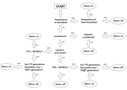
CT, CT+ 1, ..., CT+T where the price is equal to the price now. We check for theN ST following time steps how many times the device is planned to be ’on’ and how many times to be ’off’, and call them T SOn and T SOf f. Then, we sort the N ST time steps, based on the amount of own generationGt. We split the time steps in a set with the highestT SOnown generations and a set with theT SOf f lowest generations. Basically, the state should be on in theT SOntime steps with highest generation and off in theT SOf f time steps with lowest generation. Therefore, if the price is in one of the three cheapest levels ++, + or 0 and the heuristic gives off-state, we check whether the current own generation is within the set of the highest T SOngenerations. If this is the case, we switch to on-state, as the generation at this moment is higher than at least one other time step in which the state would be on. Similarly, if the price is in one of the two most expensive levels−− or −and the heuristic gives on-state, we check whether the current own generation is within the set of the lowestT SOf f generations. If this is the case, we switch to off-state, as the generation at this moment is lower than at least one other time step in which the state would be off. The flowchart for the extended heuristic is shown in Figure 4.

(32)

[image:32.595.97.533.104.411.2]

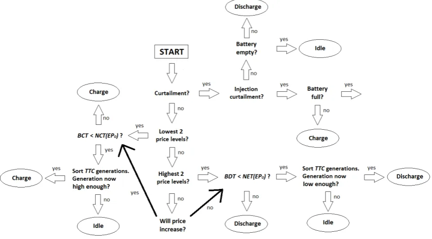
Figure 4: Flowchart for the extended thermal device heuristic.

Figure 5: Self-consumption strategy (left) versus Flexibility strategy (right) in case of low constant price level.

4.4.4 Battery