University of Warwick institutional repository: http://go.warwick.ac.uk/wrap
This paper is made available online in accordance with
publisher policies. Please scroll down to view the document
itself. Please refer to the repository record for this item and our
policy information available from the repository home page for
further information.
To see the final version of this paper please visit the publisher’s website.
Access to the published version may require a subscription.
Author(s): T. Van Doorsselaere, V. M. Nakariakov, E. Verwichte
Article Title: Coronal loop seismology using multiple transverse loop
oscillation harmonics
Year of publication: 2007
Link to published article:
http://dx.doi.org/10.1051/0004-6361:20077783
A&A 473, 959–966 (2007)
DOI: 10.1051/0004-6361:20077783
c
ESO 2007
Astronomy
&
Astrophysics
Coronal loop seismology using multiple transverse
loop oscillation harmonics
T. Van Doorsselaere, V. M. Nakariakov, and E. Verwichte
Centre for Fusion, Space, and Astrophysics, Department of Physics, University of Warwick, Coventry, CV4 7AL, UK e-mail:[email protected]
Received 3 May 2007/Accepted 2 August 2007
ABSTRACT
Context.TRACE observations (23/11/1998 06:35:57−06:48:43 UT) in the 171 Å bandpass of an active region are studied. Coronal loop oscillations are observed after a violent disruption of the equilibrium.
Aims.The oscillation properties are studied to give seismological estimates of physical quantities, such as the density scale height.
Methods.A loop segment is traced during the oscillation, and the resulting time series is analysed for periodicities.
Results.In the loop segment displacement, two periods are found: 435.6±4.5 s and 242.7±6.4 s, consistent with the periods of the fundamental and 2nd harmonic fast kink oscillation. The small uncertainties allow us to estimate the density scale height in the loop to be 109 Mm, which is about double the estimated hydrostatical value of 50 Mm.
Because a loop segment is traced, the amplitude dependence along the loop is found for each of these oscillations. The obtained spatial information is used as a seismological tool to give details about the geometry of the observed loop.
Key words.Sun: corona – Sun: magnetic fields – Sun: oscillations – Sun: UV radiation
1. Introduction
In the last decade, a wealth of oscillatory phenomena have been discovered in the solar corona (for an overview, see Nakariakov & Verwichte 2005). These oscillatory phenomena are a tool to do MHD coronal seismology with (Roberts et al. 1984).
Of particular interest are transverse coronal loop oscillations, i.e. rapidly damped oscillations of coronal loops displacing the loop axis. In recent years, they have received a lot of attention from observers and modellers alike. The oscillations are believed to be fast magnetosonic kink modes, but the mechanism respon-sible for their excitation and the rapid damping is still under debate.
These oscillatory events were first observed by Aschwanden et al. (1999); Nakariakov et al. (1999). Later on, oscillations in a sample of 17 loops were studied and analysed by Schrijver et al. (2002); Aschwanden et al. (2002). Recently, Verwichte et al. (2004) found two events with signatures of 2 different periodici-ties in a single loop in an arcade. Wang & Solanki (2004) found oscillations with a vertical polarisation, and Li & Gan (2006) observed oscillations in shrinking loops.
Fast magnetosonic kink oscillations were first studied ana-lytically by Zaitsev & Stepanov (1975). The dispersion relation for these modes was later independently derived by Edwin & Roberts (1983). To explain the damping, several theories exist: resonant absorption, wave leakage, phase mixing,. . .
Resonant absorption as a damping mechanism has re-ceived the most attention: in this mechanism a resonance is set up where the local Alfvén frequency matches the global oscillation frequency. In this resonance, energy is converted from the global mode to local Alfvén modes. Early analytical work on this mechanism was done by Goossens et al. (1995); Ruderman & Roberts (2002) and numerical modelling was done by Van Doorsselaere et al. (2004a) to extend the standard loop
model to radially inhomogeneous loops. Loop curvature was added by Van Doorsselaere et al. (2004b); Terradas et al. (2006), and longitudinal density stratification was added by Andries et al. (2005b).
Resonant absorption provides an efficient mechanism to con-vert global oscillations into localized Alfvén modes. However, observational signatures of the generated Alfvén modes, which would confirm this hypothesis, are difficult to measure.
A statistical study was performed by Ofman & Aschwanden (2002) in an attempt to pin down the damping mechanism. They concluded that the oscillations are most likely damped by phase mixing with anomalously high shear viscosity. It has not been demonstrated how phase mixing as a damping mechanism of waves in coronal loops as coherent structures would work. Also, it has yet to be demonstrated how the mechanism would operate in multi-stranded loop.
In the statistical study, however, some damping mechanisms were treated improperly, e.g. resonant absorption by assuming that the length and width of the loop are proportional to the in-homogeneity scale, (Goossens et al. 2002) and the large error bars on the observations do not currently allow to distinguish between several damping mechanisms. A larger sample size and more precise observations are needed to discriminate between damping mechanisms.
Because of inherent problems with the observational study of the solar corona (line-of-sight integration and the high den-sity contrast with the photosphere), it is practically impossi-ble to measure the coronal density and the coronal magnetic field. Some attempts to measure the density were undertaken (Aschwanden et al. 2003) and the average value of the magnetic field was estimated by Lin et al. (2000, 2004), but the error bars on the results are large.
960 T. Van Doorsselaere et al.: Coronal loop seismology throughP1/P2
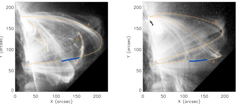
Fig. 1.Left panel: the starting frame of the studied time sequence. A indicates the oscillating loop studied in this paper. B points at the material expelled by the triggering loop (C).Right panel: the 14th frame of the studied time sequence. A indicates the oscillating loop studied in this paper. D shows another oscillating loop in the same loop complex.
Roberts et al. 1984). Coronal seismology can be achieved by studying oscillations in the corona and comparing the observed properties with models. By adjusting the model, restrictions on physical quantities in the corona can be obtained.
The transverse oscillations are an excellent tool to do coronal seismology with. The coronal dissipative coeffecients were esti-mated by Nakariakov et al. (1999) and the local magnetic field in the oscillating loop was calculated by Nakariakov & Ofman (2001). Andries et al. (2005a) used the double periodicity mea-sured by Verwichte et al. (2004) to measure the density scale height in the corona. Verwichte et al. (2006b) determined the ra-dial density structure in oscillation coronal loops, and Arregui et al. (2007) found a lower bound for the internal Alfvén transit time.
Since then, a lot of interest has gone out to multiple period-icities in the same structure. The influence of the density stratifi-cation in the corona on the ratio of the period of the fundamental and the second harmonic was studied by McEwan et al. (2006); Dymova & Ruderman (2006). Unfortunately, the only measure-ment of such a double periodicity (Verwichte et al. 2004) had very large errors and could not be used to confidently establish the density scale height. More recently, De Moortel & Brady (2007) observed a loop mainly oscillating as a 2nd harmonic, but also showing a periodicity consistent with the fundamental mode.
In this paper, we report on the high accuracy measurement of a double periodicity in a single loop. The two periods, together with the spatial structure of the oscillation, are used to determine coronal loop parameters which are difficult to measure, such as the density scale height in coronal loops.
2. Basic properties of the event
We use the 171 Å observations of the Transition Region And Coronal Explorer (TRACE) satellite (Handy et al. 1999) to study the oscillations in an active region on the 23rd of November 1998, from 06:35:57 to 06:48:43 UT. The time series has an average cadence time of 33 s.
In the images preceding the studied time series (and in Fig. 1, left), it is observed that a low lying loop is violently disrupted
(indicated by C in Fig. 1, left). After this violent event, a cloud of material is seen to escape the loop system (shown by B in Fig. 1, left), pushing aside the overlying loops (A in Fig. 1, left). Disturbed out of their equilibrium, the overlying loops start to oscillate in the wake of the escaping material. The velocity per-pendicular to the line of sight of the expelled material is es-timated to be approximately 260 km s−1, which is compatible with the values obtained by Wills-Davey & Thompson (1999); Wills-Davey (2006).
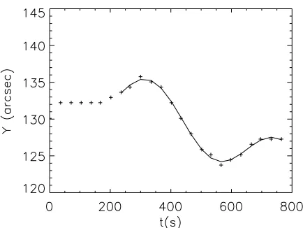
2.1. Background loop D
The loops (indicated by D in Fig. 1, right) the furthest away from the perturbation have their axis displaced during the oscillation. Because no density oscillations are observed, this suggests that they oscillate in the fundamental kink mode. The indicated loop behaves as a simple damped harmonic oscillator (see Fig. 2) with a period of 425 s and a damping time of 2300 s. The loop is estimated to be 384 Mm long (the exact procedure is described in the following paragraph).
2.2. Foreground loop A
Loop A is our main loop of interest. It has also been studied by Aschwanden et al. (2002) (case 3a). They estimated the loop length to be 390 Mm.
To estimate the length of the loop, we determine the location of the loop footpoints. Then, we measure the distance between the loop top and the mid point between the loop footpoins. We assume that this distance is the major radius of a semi-circular (toroidal) loop. The length is thenπtimes the major radius. This method for the determination of the length does not account for non-circular shape of the loop. Moreover, it is very difficult to determine the exact position of the loop footpoints. It is thus likely that the error on the estimate of the length will be substan-tial, up to 10%.
T. Van Doorsselaere et al.: Coronal loop seismology throughP1/P2 961
Fig. 2.The vertical displacement of loop D in Fig. 1, right versus time. The actual measurements are indicated with+s, while the fit is indicated with a line. The fitted period is 425 s, the damping time is 2300 s and the amplitude is 3.95 arcsec.
magnitude as in the report of Li & Gan (2006). The current loop shrinks∼17% in 12 min, and the loop in Li & Gan (2006) shrinks
∼30% in 5 min. On the other hand, Li & Gan study a short, post-flare loop, whereas the loop studied here is very long. The ap-parent shrinking of the loop may also be caused by a change of the inclination of the loop with respect to the solar surface, or a more complicated change of the loop shape.
These measured lengths are compatible with the values found by Aschwanden et al. (2002).
The loop exhibits a more involved oscillatory pattern than the background loop D. During the oscillation, a “knot” is formed near the loop top (see Fig. 1, right). If the oscillation would be a fundamental mode, the form of the loop would be main-tained (Schrijver et al. 2002). The deformation of the loop shape clearly shows that higher harmonics must be involved. On the other hand, the loop axis is still displaced, and no density os-cillations are observed. This indicates that the fast kink mode is observed, but that a combination of longitudinal mode numbers is excited. The longitudinal structure of the oscillation suggests that the 2nd harmonic kink oscillation is observed.
The brightening of the loop top by non-linear effects has been studied by Terradas & Ofman (2004) and is not considered in this paper in detail.
3. Analysis of the event
3.1. Determination of the oscillation characteristics
To facilitate the analysis, the images are rotated by 45◦ in the anti-clockwise direction. By doing this, the loop is almost aligned parallel with theX-axis (see Fig. 1). A disadvantage of this rotation is that the resolution reduces by a factor of √2, be-cause no interpolation is performed and only pixels with an even sum of indices are retained.
For a fixed horizontal coordinate (x), the vertical position of the loop (y) is estimated throughout the duration of the oscilla-tion. This procedure is repeated for 60 positions along the loop leg. The estimated perturbationsy(x,t) are indicated by a blue line in Fig. 1.
To analyse the perturbations, Gaussian noise with a standard deviation of 1.41 arcsec (i.e. 2 pixels in the rotated image) is
Fig. 3.The distribution of the fitted period to the noisy signal atx = 150.6. The mean is indicated with a+at the bottom, while the standard deviation is shown by the horizontal error bars on the mean.
added toy(x,t). Then, for a fixed vertical slit (i.e. a fixedx posi-tion), the resulting noisy data is fitted with the function
Asin
2πt
P +φ
exp (−t/τ)+C+Dt, (1)
whereAis the amplitude of the oscillation,Pthe period,φthe phase,τ the damping time andC andD describe the average intercept and global shift of the loop. For each fixedxslit, a set of{A,P, φ, τ,C,D}is obtained.
The above procedure is repeated 200 times with a varying noise. For each slit, a statistical distribution of parameters is ob-tained (e.g. Fig. 3 shows the distribution of the best-fitting period forx=150.6). From this distribution, the mean and the vari-ance can be computed (both the values are indicated in Fig. 3). We thus obtain the mean values and errors of{A,P, φ, τ,C,D}for a fixedxvalue. The fitted signal with these mean parameters is overplotted on the original data in the upper panel of Fig. 4, for
x=150.6.
Figure 5 shows the dependency of the mean parameters and their errors onx. It can be established from Fig. 5 that, for the pixels lying higher up the loop (x ∈ [135.1,156.3]), a con-sistent value for the period and phase is obtained. This suggests that the fitting identifies the same oscillation throughout that part of the loop. By averaging over the top part of the loop, a more precise estimate of the oscillation properties can be made. The errors on the oscillation properties are reduced drastically by tak-ing the mean over 31 points. For the considered interval, an aver-age period of 435.6±4.5 s is found (see the appendix for details on the error analysis), and an average damping time of 2129± 280 s. The value of the period is compatible with the previous estimates for this event (see Aschwanden et al. 2002, case 3a):
P =522 s, the value for the damping time is almost double the previously estimated value:τ=1200 s.
As a next step in the analysis, for each xposition, the best-fitted function is subtracted from the original signal. As above, the obtained residu and additional Gaussian noise is fitted with Eq. (1). Again, a statistical ensemble is found for eachxposition. Using the mean parameters, the fitted function is overplotted on the residu in the middle panel of Fig. 4.
The dependence onxof the mean fitting parameters and their errors in the residu signal is shown in Fig. 6. Again a consistent oscillation is detected in the top part of the loop. The average pe-riod found in the residu is 242.7±6.4 s, and the average damping time 872±221 s.
[image:4.595.312.531.72.174.2]962 T. Van Doorsselaere et al.: Coronal loop seismology throughP1/P2
Fig. 4.A typical signal of the transverse displacement of an oscillat-ing loop segment of one-pixel width (+), with the mean fitted signal overplotted (lines) and the trend line (dotted line). The upper panel shows the original signal, while the middle panel shows the fit to the residu. The bottom panel shows the original signal and overplots the combined fits.
3.2. Coronal loop seismology
The ratio of periods of these two oscillations can be calculated to beP1/P2 =1.795±0.051. This value significantly deviates from 2, and thus rules out the possibility of a non-linearly excited second harmonics, where the ratio has to be exactly equal to 2.
According to Nakariakov & Oraevsky (1995) the appearance of a shorter periodicity in the signal can be connected with the resonant 3-wave interaction of the longer period kink mode with a shorter period kink mode and a sausage mode. In this case, the frequency of the sausage mode would be a sum of the frequen-cies of interacting kink modes. The sausage mode in the resonant triplet would not be resolved with TRACE because of its short period. However, it is not clear whether the resonant conditions can be satisfied at all in the considered loop. Also, strictly speak-ing, the theory developed in Nakariakov & Oraevsky (1995) is only applicable to propagating waves and needs to be extended to describe the interaction between standing modes. Thus, we rule out this interpretation as theoretically undeveloped.
Long-wavelength kink modes of a magnetic cylinder are known to be weakly dispersive (e.g. Nakariakov & Verwichte 2005). The P1/P2 ratio caused by the dispersion in an un-stratified long loop is within a few percent of 2 (see Fig. 2
Fig. 5.From top to bottom:A,P,φ,τ,C,Dfor the fit of the original signal of 60 pixels along the loop leg.
in McEwan et al. 2006). The observed deviation ofP1/P2from 2 is too large to be explained by dispersion only.
The effect of the vertical density stratification (ρ(z) =
ρ0exp (−z/H)) onP1/P2was studied by Andries et al. (2005a); McEwan et al. (2006). Andries et al. assumed a vertical density stratification in the solar corona, and projected this dependency on a cylindrical loop. On the other hand, McEwan et al. took an exponential density stratification in the loop itself. Yet another approach was taken by Dymova & Ruderman (2006), who did the calculations for non-semi-circular loops in a vertically strat-ified atmosphere.
If it is assumed that the deviation ofP1/P2from 2 is solely caused by the vertical density stratification, a range of values for the relative density stratification L/πH can be found (Lis the loop length andHis the density scale height). Using the results of Andries et al. (2005a), we find a value ofL/πH=1.17+0.28
−0.3 .
Similarly, using a slightly different longitudinal density profile, McEwan et al. (2006) would findL/πH=1.08±0.28.
In the paper of Dymova & Ruderman (2006), the height of the geometry centre of the loopha is allowed to be shifted above (ha <0) or below the photosphere (ha >0). Dymova & Ruderman (2006) calculated the values forP1/P2 for different elevations of the loop above the photosphere. Their results are displayed in Fig. 7, the determined density scale height and the errors are also shown.
[image:5.595.329.560.74.392.2]T. Van Doorsselaere et al.: Coronal loop seismology throughP1/P2 963
Fig. 6.From top to bottom:A,P,φ, τ,C, Dfor the fit of the residu signal, obtained after subtraction of the fit in Fig. 5 from the original signal.
To estimate the absolute value of the density scale heightH, an estimate of the length of the loopL is needed. Before the event, the length of the loop is estimated to be 440 Mm. At the end of the observations, the loop has shortened to approximately 365 Mm. To estimate the density scale height, an average loop length of 400 Mm is assumed.
Using this average length, the estimated value L/πH = 1.17 yields a density scale height of H = 109+37
−21 Mm, us-ing the results of Andries et al. (2005a). With the results of McEwan et al. (2006), a density scale heightH = 118+41
−24 Mm
is obtained. Taking into account a non-semi-circular geometry, a valueH =109+22
−31 Mm is established. If the errorbars are in-cluded, together with the effects of a non-semi-circular geome-try, we find thatH∈[62 Mm,174 Mm]. These results are sum-marized in Table 1.
The estimates of the density scale height do not take into account the errors on the loop length. The errors on the loop length may be as large as 10%. This results in an error on the density scale height of up to 10%. For the currently estimated value forH, this would be approximately 10 Mm. This error is much less than the error induced by the uncertainties on the ratio of the periods.
The seismologically estimated value for H = 109 Mm is more than double the value of 50 Mm, expected in a hydrostati-cally stratified plasma with a temperature of 1 MK, correspond-ing to the observational bandpass 171 Å. This is not abnormal, as the stratification inside coronal loops may exceed the hydrostat-ical value by a factor of 4 (see Aschwanden et al. 2000, 2001). Even stronger, Aschwanden et al. (2000) show in their Fig. 7 that the ratio of the density scale heights in coronal loops and the
1.6 1.65 1.7 1.75 1.8 1.85 1.9 1.95 2
0 0.5 1 1.5 2 2.5 3
P1
/P
2
L/πH
ha/R=0
ha/R=0.5
ha/R=-0.5
1.6 1.65 1.7 1.75 1.8 1.85 1.9 1.95 2
0 0.5 1 1.5 2 2.5 3
P1
/P
2
L/πH 1.6 1.65 1.7 1.75 1.8 1.85 1.9 1.95 2
0 0.5 1 1.5 2 2.5 3
P1
/P
2
L/πH 1.6 1.65 1.7 1.75 1.8 1.85 1.9 1.95 2
0 0.5 1 1.5 2 2.5 3
P1
/P
2
L/πH 1.6 1.65 1.7 1.75 1.8 1.85 1.9 1.95 2
0 0.5 1 1.5 2 2.5 3
P1
/P
2
L/πH 1.6 1.65 1.7 1.75 1.8 1.85 1.9 1.95 2
0 0.5 1 1.5 2 2.5 3
P1
/P
2
L/πH 1.6 1.65 1.7 1.75 1.8 1.85 1.9 1.95 2
0 0.5 1 1.5 2 2.5 3
P1
/P
2
L/πH 1.6 1.65 1.7 1.75 1.8 1.85 1.9 1.95 2
0 0.5 1 1.5 2 2.5 3
P1
/P
2
L/πH 1.6 1.65 1.7 1.75 1.8 1.85 1.9 1.95 2
0 0.5 1 1.5 2 2.5 3
P1
/P
2
L/πH 1.6 1.65 1.7 1.75 1.8 1.85 1.9 1.95 2
0 0.5 1 1.5 2 2.5 3
P1
/P
2
L/πH 1.6 1.65 1.7 1.75 1.8 1.85 1.9 1.95 2
0 0.5 1 1.5 2 2.5 3
P1
/P
2
L/πH 1.6 1.65 1.7 1.75 1.8 1.85 1.9 1.95 2
0 0.5 1 1.5 2 2.5 3
P1
/P
2
L/πH 1.6 1.65 1.7 1.75 1.8 1.85 1.9 1.95 2
0 0.5 1 1.5 2 2.5 3
P1
/P
2
[image:6.595.304.536.76.243.2]L/πH
Fig. 7.The results from Dymova & Ruderman (2006) plotted with a dashed line (semi-circular loop, identical to Andries et al. 2005a), dot-ted line (shortened loop with centreL/π2 below the photosphere), dash-dotted line (longer loop with centreL/π2 above the photosphere). The interval forP1/P2introduced by the error bars is indicated on the
ver-tical axis with a fat dashed line. On the horizontal axis, the interval for L/πHintroduced by the non-semi-circularity is shown by a fat full line. The range forL/πHobtained by using both the errors and the non-semi-circularity is shown by a fat dashed line.
hydrostatic scale height exhibits an increasing trend for longer loops.
Our estimate may point out that coronal loops have a higher density scale height inside the loop when compared to the sur-rounding corona.
3.3. Tests of damping mechanisms
In the previous subsection, we only considered the ratioP1/P2 and did not take into account the ratio of the damping times. The ratioτ1/τ2 =2.55±0.73. This ratio is significantly higher thanP1/P2. This could point out that the damping mechanism in coronal loops is dependent on the wave number.
For a more rigorous approach, we assume that the damping time goes asCkn, whereCis a constant solely depending on the
equilibrium parameters of the loop andkis the longitudinal wave number. We can then calculate that
2.55±0.73=τ1
τ2 = k1 k2 n = 1 2 n
and thus deduce thatn=−1.35+0.49
−0.36. This interval forn accomo-dates the valuen=−1.
Alternatively, the damping time can be rescaled to the period:
τ∼Pp. Since the scaling factor can be assumed to only depend
on loop parameters, it can be established that
τ1 τ2 = P1 P2 p
, and thus thatp= log τ
1
τ2
logP1
P2
·
Using the observed values, we can estimate that p =1.60 and, taking the errors into account, has to be between 0.98 and 2.14.
These values and confidence intervals fornandpprovide a restriction on any proposed damping mechanism.
964 T. Van Doorsselaere et al.: Coronal loop seismology throughP1/P2
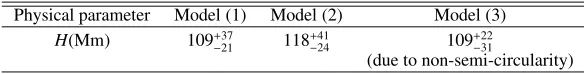
Table 1.A summary of the density scale heights in the oscillating loop, estimated using different methods. Models (1), (2) and (3) are taken from Andries et al. (2005a); McEwan et al. (2006); Dymova & Ruderman (2006) respectivily.
Physical parameter Model (1) Model (2) Model (3) H(Mm) 109+37
−21 118+ 41
−24 109+ 22
−31
(due to non-semi-circularity)
For lateral wave leakage, p is expected to be negative (Verwichte et al. 2006a), i.e. for higher harmonics, the radial ex-tent in smaller, less leakage is present and the damping time will be longer. The observationally established interval for p does not accomodate negative values. This means that, in this case, the damping cannot be explained by lateral wave leakage.
3.4. Amplitude dependence on the vertical coordinate
For a stratified medium, the fundamental mode is essentially coupled to the 3rd harmonic (see Andries et al. 2005b) without assuming a damping mechanism. The eigenfunction will thus be of the form
A(sin (θ)+asin (3θ)), (2)
whereAis the global amplitude of the fundamental harmonic,θ is the arc length along the loop (θ∈[0, π]) and the coupling pa-rameteradepends of the importance of the density stratification, measured byL/πH. Ignoring the coupling effect on the second harmonics, we expect the eigenfunction of the overtone to be
Bsin (2θ), (3)
whereBis the amplitude of the second harmonics, assumed to be independent ofAand solely determined by the form of the original perturbation.
If it is assumed that the line of sight is parallel to the loop baseline, the vertical height above the Sunzcan be written as:
z=L/πsinθ, leading to θ=arcsinπz/L.
Substituting this formula in Eqs. (2)–(3), we find the expected amplitude dependence on the vertical coordinate. For the funda-mental mode, we obtain
A
(1+3a)πz
L −4a πz
L 3
,
and for the 2nd harmonics, we find
2Bπz L
1−
πz L
2
·
However, when fitting the function for the fundamental mode to the top panel of Fig. 5, and the function for the 2nd harmonics to the top panel of Fig. 6, no conclusive results are obtained. We findA = 8.9 ±3.5 px,a = 0.02±0.36,B = −4.1 ±0.5 px,
πz0/L=0.81±0.25,πz1/L=0.56±0.25, wherez0andz1 indi-cate the position of the highest and lowest measured vertical slit, respectively. The value ofayields a range forL/πH ∈ [0,3.7] and thus reveals no extra information.
We know that the distance between z0 and z1 is exactly 30 px = 15.3 Mm. We can thus calculate that L ≈ 192 Mm, in a range ofL ∈ [79 Mm,∞[. The observationally estimated value for the length (≈400 Mm) is higher than this seismologi-cal estimate, but lies within the exorbitant errorbars.
Using a more simple approach and neglecting all coupling and higher harmonics (i.e. takeB=0 anda=0), the top panel
of Fig. 5 can be fitted with a straight line. From this fit, it is found that the amplitude will be 0 forx=82.7 arcsec. However, from the observations, it can be estimated that the footpoint is situated approximately atx=17.7 arcsec. These two values do not agree at all.
Of course, this analysis did not include the effect of a non-circular loop shape. In that case, it can be expected that a fundamental mode can still be described as
Asin (θ)+correction terms,
and that the correction terms will be smaller than the fundamen-tal mode. However, the correction terms may include a contribu-tion from the 2nd harmonic (due to the geometry), which could alter the analysis.
3.5. Alfvén speeds in the loop complex
If the measured periods in loops A and D belong to the fun-damental kink mode, the kink phase speed can be estimated in these loops. For loop A, we find a value Ck = 2L/P = 1800 km s−1. Loop D is slightly shorter, and has a slightly shorter period, so that the kink phase speed is estimated to have the same value as in loop A.
The number density is estimated to be 4.6 ×10¹⁴ m−3and 6.8×10¹⁴m−3 for, respectively, loop A and D. To measure the values, we assumed that the emission in the loop was generated in a layer of thickness 2R(the loop radiusRis measured by fit-ting the loop emission with a Gaussian) by a plasma with a fixed temperature of 0.95×10⁶ K, i.e. the peak temperature of the TRACE 171 Å filter. If the temperature of the emitting volume would be different, the plasma density would increase. As such, these estimated densities are a lower limit to the actual density. The density is then calculated byρA =
(IA−Ie)/2χR, where
IAandIeare the intensities in loop A and in the exterior plasma, respectively, andχis the TRACE 171 Å response function (taken from SolarSoft). The values for the density were not corrected for line of sight integration and are calculated in the assumption that the emitting loop is perpendicular to the line of sight.
Taking into account that the measured phase speedsCkAand
CkD and lengths of loops A and D are approximately equal to each other, we now can write down that:
1= CkA
CkD =
BA
BD
ρe+ρD
ρe+ρA ≈
BA
BD
nD
nA = 1.2BA
BD,
(4)
where quantities with subscript A and D belong to the respec-tive loop, ρe is the density outside the loops and is assumed to be small with respect to the loop densities. This assump-tion is not strictly valid for oscillating coronal loops (the inter-nal density is between 1 and 5 times the exterinter-nal density, see Aschwanden et al. 2003). In our case the value 1.2 is an upper limit to (ρe+ρD)/(ρe+ρA) and the lower limit would be 1.1 in the case ofρe=ρD.
Equation (4) can be used to estimate the ratio of the mag-nitude of the magnetic field in the two coronal loops to be
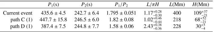
T. Van Doorsselaere et al.: Coronal loop seismology throughP1/P2 965 Table 2.A summary of periodicities, lengths and density scale heights for the events mentioned in this article. References. (1) Path C and D are measured by Verwichte et al. (2004).
P1(s) P2(s) P1/P2 L/πH L(Mm) H(Mm)
Current event 435.6±4.5 242.7±6.4 1.795±0.051 1.17+0.28
−0.30 400 109+ 37
−21
path C (1) 447.7±15.8 246.5±6.0 1.82±0.08 1.02+0.46
−0.44 218 68+ 52
−21
path D (1) 387.4±7.5 244.8±7.7 1.58±0.06 2.43+0.38
−0.36 228 30+ 5
−4
the magnetic field has roughly the same magnitude throughout different loops in the same active region.
Considering the absolute value of the magnetic field, we can state that:
10×10−4T= µρAC 2 k
2 ≤BA≤
µρAC2k=14×10−4T,
where the two outer limits are obtained in the case of a loop embedded in vacuum and a loop with density equal to the exter-nal density, respectively. These values are compatible with the value obtained by Nakariakov & Ofman (2001); Verwichte et al. (2004). The outer limits obtained above do not take into account the errors on the density measurement, and merely indicate the errors introduced by the unknown density contrast between the internal of the loop and the external plasma.
The results in this subsection have to be taken with caution: the errors on both the density and, to a lesser extent, the length are large. As such, the values found in this subsection are only an indication of the order of magnitude of the physical quantities.
4. Verwichte et al. (2004) revisited
In the currently studied event, the measurement errors on the pe-riods were drastically reduced by averaging the period over a whole segment of the oscillating loop. A loop segment was also studied by Verwichte et al. (2004), but a different averaging for-mula was used, based on the standard deviation of the data cloud rather than the averaging of the measurement errors. However, when redoing the analysis and using Eqs. (A.1)–(A.2), a more precise determination of the periods is obtained.
Their path C now hasP1=447.7±15.8 s andP2 =246.5± 6.0 s, leading to P1/P2 = 1.82 ± 0.08. Using the model of Andries et al. (2005a), we find L/πH = 1.02+0.46
−0.44. Using the lengthL = 218 Mm of that loop, a density scale height H =
68+52
−21Mm is obtained.
Similarly, their path D shows periodicities P1 = 387.4 ± 7.5 s andP2 =244.8±7.7 s, resulting inP1/P2 =1.58±0.06 andL/πH =2.43+0.38
−0.36. Together with the estimated lengthL = 228 Mm, we find a density scale heightH=30+−54Mm.
These values for the density scale height differ strongly from the value we obtain in the currently studied event. This fact, how-ever, is compatible with Fig. 7 in Aschwanden et al. (2000). That graph shows that the scale height in shorter coronal loops (as is the case in Verwichte et al. 2004) is expected to be lower than for longer coronal loops (current event). Also, the loops studied by Verwichte et al. (2004) are post-flare loops and may not have settled into equilibrium.
A summary of all the periods, lengths and density scale heights of the events studied in Verwichte et al. (2004) and the current paper is given in Table 2.
5. Conclusions
In this article, TRACE 171 Å observations of an active region were analysed. By tracing out a loop segment, two oscillation periods could be detected with high confidence: 435.6 ±4.5 s and 242.7 ±6.4 s. Using these periods, and interpreting them as the fundamental and the 2nd harmonic oscillation, a value
P1/P2=1.795±0.051 was found.
This value allowed us to establish L/πH = 1.17, and lead to a density scale height of H = 109+37
−21 Mm. Such a value for the density scale height in the loop is significantly higher than the hydrostatically expected value (50 Mm). Our result thus suggests that the density scale height in coronal loops is much higher than that in the surrounding corona, a result also found by Aschwanden et al. (2000).
We used the measurements for the damping times to study the viability of different damping mechanisms. We were able to find that the damping time must be approximately inversely pro-portional to the wave number. By relating the ratio of damping times and periods, we found thatτ ∼P1.60. Using the relations between the damping time, the wave number and the period, we have established that the observed damping times can be ex-plained by resonant absorption and not by lateral wave leakage. Furthermore, we estimated that the magnetic field in the ob-served loop is between 10 and 14 G and thus in the same range as Nakariakov & Ofman (2001). By comparing the observed os-cillation with an osos-cillation in a neighbouring loop in the same active region, we were able to establish that the ratio of the mag-netic fields is between 1.1 and 1.2. This suggests that, for loops with a similar length, the magnetic field remains almost constant throughout an active region.
We used the eigenfunction to obtain geometrical properties of the loop, but found that the observational errors are to large to achieve this. A loop length L = 192 Mm in a range of [75 Mm,∞[ was estimated. This value ofL is not close to the observed loop length, but lies within the errorbars.
Lastly, we revisited the results of Verwichte et al. (2004) and used a different statistical method to reduce the errors on the measurements of the periods. For those events, density scale heights ofH = 68+−5221Mm andH = 30+−54 Mm are thus found. These values differ significantly from the value found in our event. This fact, however, is compatible with the findings of Aschwanden et al. (2000).
Acknowledgements. T.V.D. would like to acknowledge the financial support of PPARC.
Appendix A: Estimates of errors
To calculate the errors on the mean periods, it was assumed that all fitted estimates of the periodPi = P(x = i) along the loop
were taken from a Gaussian distribution with a variance of (σi)2. Statistical analysis states that the mean periodPis calculated as:
P= N−1
i=0 P
i/
(σi)2 N−1
i=0 1/(σi)2
966 T. Van Doorsselaere et al.: Coronal loop seismology throughP1/P2 The error on the mean can be calculated by:
σ2
P=
1 N−1
i=0 1/(σi)2
· (A.2)
The errors ofP1/P2can be calculated by:
σP1/P2
P1/P2 2
=
σP1
P1 2
+
σP2
P2 2
,
if it is assumed that the errors onP1andP2are uncorrelated.
References
Andries, J., Arregui, I., & Goossens, M. 2005a, ApJ, 624, L57
Andries, J., Goossens, M., Hollweg, J. V., Arregui, I., & Van Doorsselaere, T. 2005b, A&A, 430, 1109
Arregui, I., Andries, J., van Doorsselaere, T., Goossens, M., & Poedts, S. 2007, A&A, 463, 333
Aschwanden, M. J., Fletcher, L., Schrijver, C. J., & Alexander, D. 1999, ApJ, 520, 880
Aschwanden, M. J., Nightingale, R. W., & Alexander, D. 2000, ApJ, 541, 1059 Aschwanden, M. J., Schrijver, C. J., & Alexander, D. 2001, ApJ, 550, 1036 Aschwanden, M. J., De Pontieu, B., Schrijver, C. J., & Title, A. M. 2002,
Sol. Phys., 206, 99
Aschwanden, M. J., Nightingale, R. W., Andries, J., Goossens, M., & Van Doorsselaere, T. 2003, ApJ, 598, 1375
De Moortel, I., & Brady, C. S. 2007, ApJ, Accepted Dymova, M. V., & Ruderman, M. S. 2006, A&A, 459, 241 Edwin, P. M., & Roberts, B. 1983, Sol. Phys., 88, 179
Goossens, M., Ruderman, M. S., & Hollweg, J. V. 1995, Sol. Phys., 157, 75 Goossens, M., Andries, J., & Aschwanden, M. J. 2002, A&A, 394, L39 Handy, B. N., Acton, L. W., Kankelborg, C. C., et al. 1999, Sol. Phys., 187, 229 Li, Y. P., & Gan, W. Q. 2006, ApJ, 644, L97
Lin, H., Penn, M. J., & Tomczyk, S. 2000, ApJ, 541, L83 Lin, H., Kuhn, J. R., & Coulter, R. 2004, ApJ, 613, L177
McEwan, M. P., Donnelly, G. R., Díaz, A. J., & Roberts, B. 2006, A&A, 460, 893
Nakariakov, V. M., & Ofman, L. 2001, A&A, 372, L53 Nakariakov, V. M., & Oraevsky, V. N. 1995, Sol. Phys., 160, 289 Nakariakov, V. M., & Verwichte, E. 2005, Living Rev. Sol. Phys., 2, 3 Nakariakov, V. M., Ofman, L., DeLuca, E. E., Roberts, B., & Davila, J. M. 1999,
Science, 285, 862
Ofman, L., & Aschwanden, M. J. 2002, ApJ, 576, L153 Roberts, B., Edwin, P. M., & Benz, A. O. 1984, ApJ, 279, 857 Ruderman, M. S., & Roberts, B. 2002, ApJ, 577, 475
Schrijver, C. J., Aschwanden, M. J., & Title, A. M. 2002, Sol. Phys., 206, 69 Terradas, J., & Ofman, L. 2004, ApJ, 610, 523
Terradas, J., Oliver, R., & Ballester, J. L. 2006, ApJ, 642, 533 Uchida, Y. 1970, PASJ, 22, 341
Van Doorsselaere, T., Andries, J., Poedts, S., & Goossens, M. 2004a, ApJ, 606, 1223
Van Doorsselaere, T., Debosscher, A., Andries, J., & Poedts, S. 2004b, A&A, 424, 1065
Verwichte, E., Nakariakov, V. M., Ofman, L., & Deluca, E. E. 2004, Sol. Phys., 223, 77
Verwichte, E., Foullon, C., & Nakariakov, V. M. 2006a, A&A, 449, 769 Verwichte, E., Foullon, C., & Nakariakov, V. M. 2006b, A&A, 452, 615 Wang, T. J., & Solanki, S. K. 2004, A&A, 421, L33
Wills-Davey, M. J. 2006, ApJ, 645, 757
Wills-Davey, M. J., & Thompson, B. J. 1999, Sol. Phys., 190, 467