Education and work

Philip Trostel and Ian Walker*

Department of Economics University of Warwick

Coventry, CV4 7AL

March 2000

Abstract

This paper examines the linkage between the incentives to work and

to invest in human capital through education. These incentives are

shown to be mutually reinforcing in a simple stylized model. This

theoretical prediction is investigated empirically using three large

micro datasets covering a broad set of countries. As one might

expect, education and work are strongly (positively) correlated.

This correlation has important implications for models of fiscal

policy and economic growth. It also has important implications for

the estimation of labor supply and the rate of return to education.

JEL Codes: J22,I20

*_{We are grateful to the European Union Targetted Socio-Economic}

1_{A partial list of these studies is Lucas (1988, 1993), Lord}

(1989), Becker et al. (1990), King and Rebelo (1990), Davies and Whalley (1991), Tamura (1991), Ehrlich and Lui (1991), Jones and Manuelli (1992), Glomm and Ravikumar (1992, 1997), Nerlove et al. (1993), Mulligan and Sala-i-Martin (1993), Caballé and Santos (1993), Barro and Sala-i-Martin (1995), De Gregorio (1996), Mino (1996), Dupor et al. (1996), Kaplow (1996), Steurle (1996), Agell and Lommerud (1997), Perroni (1997), Kim (1998), Lin (1998), and Lord and Rangazas (1998).

This paper examines the linkage between the level of education

and subsequent time spent working. A s o n e m i g h t e x p e c t , a

mutually-reinforcing correlation is found both theoretically and

empirically. In addition to being interesting in its own right

because of its implications for education and employment policies,

the finding that education and work decisions are mutually

reinforcing has at least three important implications.

First, it casts doubt on the applicability of the

"wealth-maximizing" models of human capital accumulation. Economic models

which incorporate human capital creation have become increasingly

common over the past decade. Most of these models have been

simplified by assuming that leisure time is fixed.1 _{By ignoring the}

choice between work and leisure these wealth-maximizing (as opposed

to utility-maximizing) models focus exclusively on the choice between

work and education. The results in this paper, however, decisively

reject the notion that the work/training choice is independent of the

work/leisure choice. Moreover, recent research has shown that the

interdependency between the work/training and work/leisure choices

may be important in some analyses. Trostel (1993) found that the

interdependency between human capital investment and subsequent work

is crucial in the debate over the extent that taxation affects human

2_{This is also found in Jones et al. (1993), Mendoza et al.}

(1997), and Milesi-Ferretti and Roubini (1998).

3_{See Blundell and MaCurdy (forthcoming) for a recent survey of}

this literature. See also Killingsworth (1983), Killingsworth and Heckman (1986), and Pencavel (1986).

4_{This point applies not just to structural models of labor}

supply, such as Mroz (1987), but also to difference-in-differences models, such as Blundell et al. (1998).

5_{Shaw (1996) makes an analogous argument concerning the effect}

of on-the-job training on estimates of labor supply.

6_{Our very preliminary investigation has indeed found that the}

estimated labor supply elasticity is understated when education is taken as exogenous, although not by a large amount.

7_{See Ashenfelter et al. (2000), Card (1995), and Psacharopoulos}

(1994) for recent surveys of this literature.

this interdependency may be crucial in the debate over the extent

that taxation affects economic growth.2 _{These earlier results}

coupled with the findings in this paper show that the frequent

simplifying assumption of constant leisure can be an important

restriction in human capital models.

Second, empirical research on labor supply3 _{has ignored the}

interaction between the work/education and work/leisure choices. The

level of education is treated as an exogenous variable in the

estimation of labour supply elasticities (either explicitly or

implicitly by splitting the sample by education level). In other

words, education is implicitly assumed to affect the rate of pay, but

not hours of work.4 _{In a full life-cycle perspective, however,}

education is endogenously determined along with hours of work.

Therefore, estimates of labour supply elasticities may be biased

and/or inefficient.5 _{To be specific, it is likely that estimates of}

the wage elasticity are understated.6

8_{This sample-selection bias is related to, but distinct from,}

censoring or "composition" bias, which appears to be very small [see, e.g., Dearden (1999)].

9_{These issues have been addressed to a small extent in the}

rate-of-return literature. For example, Ashenfelter and Ham (1979) and Nickell (1979) estimate the risk-adjusted rate of return to education by accounting for unemployment. Some studies, e.g., Mincer (1974), have included weeks of work (assumed exogenous) in their earnings equations. But it does not appear that these issues have been fully appreciated. Our very preliminary examination of this issue suggests that it causes a non-trivial downward bias in the estimated of rate of return to education.

may also be biased and/or inefficient because it fails to account for

the endogenous interaction between education and hours worked. In

particular, studies which use the wage rate as the dependent variable

typically do not account for the endogeniety of participation and may

therefore be subject to sample-selection bias.8 _{The potential for}

sample-selection bias is smaller in studies which use annual earnings

as the dependent variable, but in this case endogenous variation in

conditional hours of work is not accounted for.9

This paper uses a simple two-period model to show that

education and work choices are mutually reinforcing under likely

circumstances. This prediction is then supported empirically using

individual-level data from the U.S. Current Population Survey, the

British Family Resources Survey, and the International Social Survey

Programme. This conclusion is robust to including the wage rate

directly into the hours equation.

Specifically, these datasets show that, for working-age men,

one additional year of education is associated with roughly an

additional 0.9 to 1.3 hours of work per week. Not surprisingly, the

correlation is even stronger for women. Working-age women work

10_{See also Ghez and Becker (1975), Heckman (1976), Ryder et al.}

(1976), Weiss and Gronau (1981), Killingsworth (1983), and Killingsworth and Heckman (1986).

of schooling. Most, but not all, of this correlation occurs on the

extensive margin, that is, through differences in the probability of

working. For men (women), the probability of working increases by

roughly 1.6 to 2.6 (3.4 to 3.8) percentage points per year of

education. A significant negative correlation between education and

unemployment is an important part of the story; but most of the

correlation between education and employment comes from the negative

correlation between education and labor-force participation. For

working-age men (women), an additional year of education is

associated with a 0.8 to 1.5 (3.1 to 3.5) percentage point lower

probability of being out of the labor force. Moreover, owing to the

large sample sizes, these effects are very precisely estimated. And,

although there is a fair amount of variation in these correlations

across 27 countries in the International Social Survey Programme, the

same general pattern is found in practically every country.

Before proceeding to the analysis it should be acknowledged

that many of the findings of this study are implicit in many earlier

studies. The idea that education and work choices are mutually

interdependent ex ante is clearly demonstrated in Blinder and Weiss

(1976).10 _{The original contribution of the theory presented in the}

next section is that the interdependence between education and work

choices is examined explicitly and in depth. Moreover, the

specification of human capital is more general in an important

dimension than those used in previous theoretical work. A positive

11_{See, e.g., Mincer (1974), Ghez and Becker (1975), Pencavel}

(1986), Killingsworth and Heckman (1986), Eckstein and Wolpin (1989), Becker (1993), Ríos-Rull (1993), Card (1994), Phelps and Zoega (1997), and Blau (1998).

12_{The important restriction imposed in a two-period framework is}

that it does not capture potential intertemporal substitution of leisure within each period. As will become apparent below, except for in a special case, the opportunity cost of leisure changes over time as the human capital stock evolves, which creates an incentive to substitute leisure intertemporally. This possibility reinforces the mutual reinforcement of human capital and work decisions shown below.

13_{It is not even clear that investment in human capital is}

risky. There is considerable evidence that investment in education reduces income risk by reducing the probability of unemployment.

This evidence is surveyed in Trostel, Perroni, and Walker (1998). previously.11 _{The previous empirical work, however, did not}

explicitly explore the interaction between schooling and labour

supply (this interaction was not the primary focus in the earlier

work). In other words, although the interaction between years of

education and subsequent hours of work has been indicated in previous

theoretical and empirical work, this is the first study to explore

it, and its implications, in depth.

2 Theory

2.1 The Model

The basic intuition can be shown most easily in a two-period

model with no uncertainty. A two-period framework simplifies the

analysis considerably, but it is sufficient to model the essence of

the decisions to work and to invest in human capital from

education.12 _{Ignoring uncertainty also simplifies the analysis,}

particularly because it is not clear how investment in human capital

14_{Non-time inputs in the production of human capital are not}

important in this context and for simplicity are ignored. education because of the lack of data on on-the-job training.

Moreover, education is likely to be the most important type of human

capital for most workers.

Individuals are assumed to be endowed with one unit of time per

period, t, which is allocated among three alternatives: working, l,

schooling, s, and leisure,

R

(1) 1

/

R

As mentioned earlier, more often than not, models with human capital

accumulation have been simplified by assuming

R

Time allocated to schooling in the first period produces human

capital, H, which increases earnings from working in the second

period.14 _{Thus the wage rate, w, in the second period is}

(2) w₂ = H(s₁)w₁, H(0)

/

Human capital production is assumed to be governed by a simple

isoelastic function:

(3) H(s) =

N

F

where

N

F

scale in producing human capital. To produce an interior solution

(i.e., l₁, s₁ > 0), diminishing returns in human capital production

is assumed.

It is worth emphasizing that the first period in this model is

not just the schooling age, but is the entire first half of economic

with the fact that most young people initially specialize completely

in producing human capital. Full-time schooling ends long before

middle age. Similarly, the second period in this model is not just

the working age. The second period also includes retirement age, and

variation in the age of retirement is one of the ways that work can

vary in the second period.

A frictionless financial market is assumed which allows

individuals to save or borrow at rate r in the first period. An

initial financial endowment, e, is assumed. Bequests are ignored (or

e can be interpreted as the initial endowment less the present value

of the future bequest). Thus the budget constraint is

(4) (1+r)e + (1+r)w1l1 + w2l2 = (1+r)c1 - c2,

where c is consumption per period.

Utility, U, is a function of consumption and leisure in each

period. Human capital produced in the first period is assumed to

increase the productivity of leisure, v, in the second period. Thus

the utility function is

(5) U = U(c₁,c₂,

R

R

D

/

where

D

a simple isoelastic function:

(6) v(H) = H", 1

$

"

$

"

Most modelling of human capital ignores its potential impact on

the productivity of leisure time (i.e.,

"

/

15_{More recently, Killingsworth and Heckman (1986), Rebelo}

(1991), Stokey and Rebelo (1995), Mendoza et al. (1997), Ortigueira and Santos (1997), and Milesi-Ferretti and Roubini (1998) have used this specification.

16_{Becker (1965) makes a this argument in a similar context.}

(1976),15 _{human capital has sometimes been assumed to affect the}

productivity of leisure in the same proportion that it affects the

productivity of work (i.e.,

"

/

specification of human capital, however, may be no less restrictive

than the usual specification. In other words, neither of the special

cases used in the literature appears particularly likely. It does

seem likely that human capital will affect the productivity of

leisure time to some extent. Indeed, Michael (1972) provides some

empirical evidence that education affects the productivity of

leisure. But it seems unlikely that human capital affects the

productivity of work and leisure in the same proportion. Because

there is much less scope for specialization, limits on leisure

productivity seem much more likely than limits on work

productivity.16 _{Moreover, the extent that human capital affects the}

productivity of leisure is crucial for the interaction between human

capital and hours of work. Thus a general specification is assumed.

2.2 The Equilibrium Relationship between Education and Work

The equilibrium relationship between investment in education

and expected future hours of work can be easily deduced from the

first-order conditions of the individual's optimization problem

(assuming, of course, that the budget constraint is continuous).

Specifically, maximizing (5) by the choices of c₁, c₂, s₁, l₁, and l₂

-(4) and (6) yields the following first-order conditions:

(7.1)

M

M

8

(7.2) (1+

D

M

M

2 -

8

(7.3) -

M

MR

D

"FN

R

M

MR

8FN

(7.4) -

M

MR

8

(7.5) - (1+

D

M

MR

2 +

8

(7.6) (1+r)e + (1+r)wl1 + wHl2 - (1+r)c1 - c2 = 0,

where

8

been left off of s and w and are understood to be their first-period

values.

Combining first-order conditions (7.3) - (7.5) shows the

equilibrium relationship between education and work:

(8) s = [

FN

"

"

This equation reveals that the relationship between education and

future work is weakly positive. Unless human capital from education

affects the productivity of leisure time and the productivity of work

time proportionately (i.e.,

"

between education and work. Moreover, this relationship is

independent of preferences about work, consumption, and discounting.

Equation (8) shows a no-arbitrage condition rather than a preference

relationship.

The intuition for this result is straightforward. First

conditions (7.3) and (7.4) shows that the marginal return on

investment in education is equated to the rate of return on financial

assets:

(9)

FN

This equation shows that l2 affects the rate of return on investment

in human capital. Expected future hours of work is the utilization

rate of human capital. Thus l2 directly affects the rate of return

on investment in human capital and the incentive to invest in

education.

When the productivity of leisure is affected by human capital,

however, increases in work increase the market utilization of human

capital while decreasing its nonmarket utilization. In the neutral

specification (

"

sectors proportionately, the overall utilization of human capital is

unaffected by future work, thus s and l₂ are independent. This

independence property makes the neutral special case much easier to

analyze than the general case. Thus it is a somewhat common simple

alternative to wealth-maximizing specification.

2.3 The Effect of Education on Subsequent Work

At first glance it might seem that the effect of education on

subsequent labor supply is ambiguous. Investment in human capital

increases the wage rate, and increases in the wage rate produce

opposing income and substitution effects on hours of work. The

higher wage rate, however, is only part of the story of how

investment in education affects later labor supply.

is treated as an exogenous parameter in this section. The analysis

in this section is simplified considerably by imposing the

simplifying assumptions that human capital does not affect the

productivity of leisure (i.e., the typical specification where

"

0), and that utility is separable in its four arguments (i.e., uij =

0

œ

…

The labor supply response to education, dl2/ds, is derived by

totally differentiating the first-order conditions of the

individual's optimization problem with s treated as exogenous.

Totally differentiating (7.1) - (7.2) and (7.4) - (7.6), applying

Cramer's Rule, and simplifying yields

dl2

8FN

D

(10) = +

ds (1+

D

*

*

Hw2_U2

ccURR[

FN

(1+

D

*

*

where

*

*

associated with the maximization problem. If s is at its optimal

value, then the second expression in (10) is zero (see FOC (7.3) and

(7.4)). The second-order condition requires that

*

*

dl₂/ds > 0.

The labor-supply responses to the wage rate and income (i.e.,

dl₂/dw and dl₂/de) can be derived in an analogous manner. Comparing

the terms in these equations to the terms in equation (10) reveals

that s affects l₂ in four ways. In fact, equation (10) can be

rewritten as

%dl₂

8F

cc

0

F

(11) =

0

F

17_{This can be shown by comparing dl}

2/ds to dl2/d

T

T

/

d(w₂/w₁)|_dU=ds=0. In fact, dl₂/ds and dl₂/d

T

both induce static substitution effects, offsetting static income effects, and an intertemporal substitution effect. In other words, the effect of education on work is conceptually similar to an intertemporal substitution of life-cycle labor supply (note that this is intertemporal substitution is over, say, 25 year periods and not annual periods as emphasized in the real business cycle literature). where

0

supply, and

0

four terms in (11) correspond to the four terms in (10).

Equation (11) reveals that the way education affects labor

supply is not simply that it causes opposing income and substitution

effects from a higher wage rate. The higher wage rate in the second

period does cause the usual static substitution and income effects

(these are the first and third terms). Education also causes two

additional effects. First, schooling reduces earnings in the first

period. Thus there is a negative income effect in the first period

(this is the fourth term). When s is optimally chosen the two income

effects exactly offset each other (because the marginal return equals

the marginal cost). Second, the higher wage in the second period

relative to the first period also induces an intertemporal

substitution effect toward more work in the second period (this is

the second term).17 _{Thus, equation (11) shows that when s is at its}

optimal level, s induces two unambiguous substitution effects on l₂

(assuming, of course, that human capital affects the productivity of

leisure less than it affects the productivity of work).

3 Evidence

The previous section demonstrated that education and work

18_{The FRS is a large continuous survey of British households}

administered by the (U.K.) Department of Social Security and is designed for tax and social security analysis. It contains high-quality data on all sources of income. See Department of Social Security (1997).

if this result and its potential implications discussed in the

Introduction are economically important. Thus, the economic

importance of this theoretical result is investigated below.

3.1 The Data

We use three large micro datasets: the 1991 merged outgoing

rotation group file of the U.S. Current Population Survey, CPS (1991

was the last year that education was measured as years of schooling

as opposed to a credential-based measure); the pooled 1994-98 British

Family Resources Survey, FRS;18 _{and the pooled 1989-95 International}

Social Survey Programme, ISSP. The ISSP is a continuing annual set

of cross-national surveys covering various social research topics.

It contains comparable data from 33 countries (27 of these have

complete labor-market data) over the period 1985 through 1995,

although many of the countries participated only in a few of the

later years. Data from the years prior to 1989 were not used because

they lacked complete information on labor force participation.

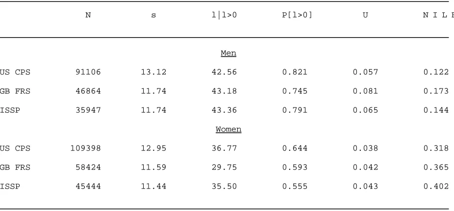
All samples are restricted to those aged 25 to 64 inclusive,

not in school, not self-employed, with less than 21 years of

education, and without missing information on education or labor

force status. Table 1 gives the most relevant summary statistics for

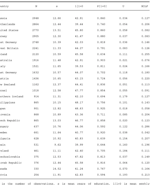
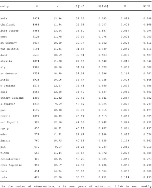
the three datasets. Tables 2 and 3 give the summary statistics for

the individual countries in the ISSP.

19_{We would have preferred to use a Heckman two-stage approach,}

but we have been unable to find exogenous variables in our datasets to separately identify the selection equation.

20_{In all the regressions in Table 4 there are unreported}

controls for a fourth-order age polynomial and for: race and interview month in the CPS, each of the 51 interview months in the FRS, and each year in each country in the ISSP.

datasets are collapsed by the level of education. Figures 1 and 2

show the raw correlation between (unconditional) weekly hours of work

and education for men and women. Figures 3 and 4 illustrate the raw

relationship between schooling and weekly hours of work conditional

on being employed. And Figures 5 and 6 show the raw correlation

between working rates and years of schooling for men and women.

These figures reveal a positive raw correlation between education and

labor supply. That is, the idea that education and work are mutually

reinforcing is found in the unconditioned data. This idea is now

formally tested on the micro data.

3.2 The Correlation Between Education and Work

Hours of work are truncated at zero, thus OLS residuals are

non-normal and the coefficient estimates can be biased and

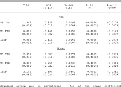
inconsistent. Thus a tobit procedure is used.19 _{Tobit estimates of}

the correlation between education and weekly hours of work are

reported at the left of Table 4.20 _{The results confirm the}

theoretical prediction and the impression shown in Figures 1 and 2.

They reveal a precisely-estimated positive correlation between

education and work. The largest correlations in the three datasets

are found in the U.S. CPS. For men (women), each year of education

is associated with an additional 1.35 (2.36) hours of work per week.

21_{There are unreported controls for a fourth-order age}

polynomial and for each year.

education is associated with an additional 0.87 (2.09) hours of work

per week. The correlations in the pooled ISSP are closer to that in

Britain. In addition to being highly statistically significant,

these correlations are economically huge. These coefficients are

between 2.6% to 3.8% of the sample means for men, and between 10% to

11.9% of the sample means for women. That is, one additional year

of education is associated with about 3% (11%) more work for men

(women).

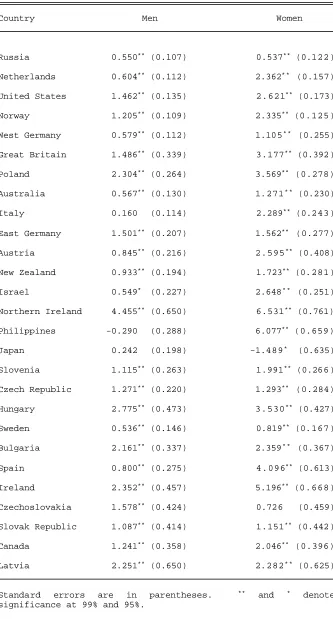
Tobit estimates of the correlation between education and weekly

hours of work for the separate countries in the ISSP are reported in

Table 5.21 _{Although there is a fair amount of variation in the}

coefficients across the countries, they show the same general

pattern. The estimated coefficient on education is positive and

statistically significant at the 99% level in 23 of the 27 countries

for men, and in 25 countries for women. Japan is the only country

which does not display a statistically-significant positive

correlation for either men or women. This table reveals that

positive correlation between education and work emerges despite wide

variation in the degree of economic development, culture, labor

market policies, etc.

It must be emphasized, however, that the estimated coefficient

of schooling on work should not be interpreted as a causal effect.

The level of education is predetermined when work decisions are

observed (except for perhaps an extremely small proportion of

observations). But, as stressed earlier, the level of education is

22_{We also have run seemingly-unrelated regressions of education}

and work. These regressions perform well and show a very strong positive correlation between their residuals (indicating that schooling and work affect each other). These results do not add any additional insight, however, and are not reported. To isolate the causal effect of education would require a two-stage instrumental-v ariable approach, but it is difficult to conceiinstrumental-ve of instrumental-val i d instruments in this context.

23_{A negative correlation on the conditional-hours margin is not}

necessarily inconsistent with the theory and the other empirical correlations. It is possible, perhaps even likely, that those which are subject to higher unemployment risk and/or more likely to retire early (i.e., those with less education) will work longer hours when employed. In other words, intertemporal substitution is likely to reduce the correlation on the condition hours margin, possibly enough to make it negative. On intertemporal substitution of work, see, for example, Altonji (1986), Ham (1986), and Card (1994).

work are likely to be very closely correlated with anticipated levels

of work, and anticipated work should affect the chosen level of

education. Thus the coefficient should be interpreted as estimate

of the equilibrium relationship, and not the causal effect.22

3.3 The Intensive Margin

Table 4 also reports OLS estimates of the correlation between

conditional weekly hours of work and education. Not surprisingly,

the correlation is much smaller. In other words, as stressed in

Heckman's (1993) survey of empirical labor research, most of the

action occurs on the extensive rather than the intensive margin.

Conditional on being employed, each year of education is associated

with an additional 0.32 (0.39) hours of work for men (women) in the

CPS. The corresponding numbers in the pooled ISSP are smaller, 0.012

(0.19). Paradoxically, the corresponding numbers in the FRS are both

much smaller and much larger. For British men, the relationship is

reversed; there is a large and statistically-significant negative

24_{There are unreported controls for a fourth-order age}

polynomial and for each year.

British women, there is an even larger positive correlation between

education and conditional hours.

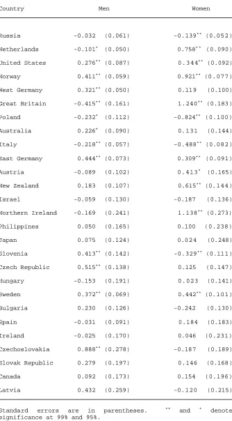
OLS estimates of the correlation between education and

conditional weekly hours of work for the separate countries in the

ISSP are given in Table 6.24 _{Again, the results for the individual}

countries are consistent with those found in the large datasets. The

conditional correlations between work hours and schooling are much

weaker than the unconditional correlations. In fact, in many cases

[11 (7) of the 27 for men (women)] there is a negative correlation

in the conditional-hours dimension. There is a positive and

statically-significant correlation in only 9 (10) of the 27 countries

for men (women). There are also a few statistically-significant

negative correlations (4 for men, and 3 for women). Overall,

however, there is more evidence for a positive correlation. There

are negative correlations for both men and women in only 3 countries

(compared to 12 countries that have positive correlations for both

men and women). Table 6 also confirms that Britain is indeed unusual

in this dimension. Both the largest negative coefficient for men and

largest positive coefficient for women occur in Britain.

3.4 The Extensive Margin

Probit estimates of the correlation between employment and

education are also presented in Table 4. There is an

economically-huge correlation between employment and education. For American men,

one additional year of education is associated with a 2.0 percentage

25_{See, e.g., Mincer (1974, 1993), Ashenfelter and Ham (1979),}

Nickell (1979), Becker (1993), Nickell and Bell (1996), and Phelps and Zoega (1997).

corresponding number is 2.6 percentage points. And in the pooled

ISSP, the figure is 1.6 percentage points. For women, one additional

year of education is associated with a higher probability of

employment of 3.7 percentage points in the CPS, 3.4 percentage points

in the FRS, and 3.8 percentage points in the pooled ISSP.

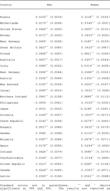
Probit estimates for the individual countries in the ISSP are

reported in Table 7. They reveal a similar picture. For men

(women), there is a significant positive correlation between

employment and education in 24 (26) of the 27 countries. Moreover,

for men (women), an extra year of education is associated with at

least a one percentage point higher probability of employment in 20

(26) countries.

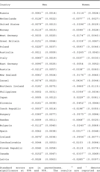
The last two columns in Table 4 report the correlations between

unemployment and education and between not-in-the-labor-force and

education. These cases show that most of the correlation between

employment and schooling comes from the correlation between

labor-force participation and schooling, especially for women.

As shown in numerous previous studies,25 _{there is a}

statistically-significant negative correlation between unemployment

and education. For men, an extra year of education is associated

with about a half percentage point reduction in the probability of

unemployment in the CPS and pooled ISSP, and a one percentage point

reduction in the FRS. For women, each year of education associated

with about a quarter percentage point reduction in the probability

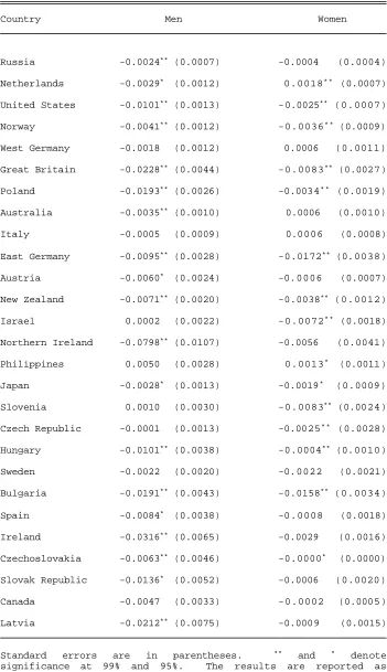
There is much more variation in the unemployment-schooling

coefficient in the separate ISSP country probits shown in Table 8.

But the general pattern is consistent with that found in the large

datasets. In particular, the coefficient is negative in 24 of the

27 countries for men (and significant in 19), and in 22 countries for

women (and significant in 13 of these). The Philippines is the only

country where the correlation is positive for both men and women.

Table 8 also confirms that in unemployment dimension, unlike in all

the other dimensions, the correlations are generally stronger for men

than women. The men have a larger negative correlation in 21 of the

27 countries.

The strongest correlation between education and work occurs in

the not-in-the-labor-force dimension, particularly, and not

surprisingly, for women. Each year of schooling is associated with

a 1.2, 1.5, and 0.8 percentage point reduction in the probability of

being out of the labor force in the CPS, FRS, and pooled ISSP,

respectively. For women, the negative correlations are between 3.1

and 3.4 percentage points per year of schooling.

Table 9 reports the correlations between not-in-the-labor-force

and education for the separate countries in the ISSP. For men, there

is a negative correlation in every country (and statistically

significant in 18 of the 27 countries). For women, the correlation

is negative in 26 of the 27 countries (and significant in 23 of

those). The negative correlation is larger for women than men in 25

countries.

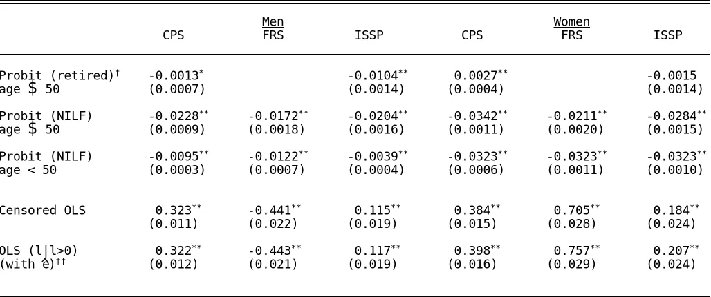
3.5 Some Sensitivity Analysis

26_{See, e.g., Gustman and Steinmeier (2000).}

Three additional probits are reported to demonstrate that the

positive link between education and work also operates on the

retirement dimension. The not-in-the-labor-force probits reported

previously included those classified as retired. Part of the reason

for counting retired as not-in-the-labor-force is dictated by the

data. The FRS does not have a separate retired category. The CPS

measure of retired is not consistent with the measures that we use

for weekly hours and not-in-the-labor-force. There are also some

anomalies in the ISSP measure of retired. But more importantly, the

classification of retirement is arbitrary.26 _{For instance, most}

older women not in the labor force are not counted as retired

obviously because they have not worked recently.

The top row of Table 10 reports the probits of retirement on

schooling. The coefficient estimates are negative and significant

for men, negative and insignificant for women in the ISSP, but

positive and significant for women in the CPS. As mentioned above,

however, we do have much faith in the retirement measures, especially

for women. Thus, in the second row of Table 10 we report

not-in-the-labor-force probits for those aged 50 and above. Presumably this

removes the arbitrary retirement distinction. For comparison

purposes not-in-the-labor-force probits for those under the age of

50 are presented in the third row. These probits show that the

correlation between schooling and labor force participation is higher

for men above the age of 50, confirming that the positive link

between education and work occurs through early retirement as well

somewhat weaker for those over 50 in the FRS and pooled ISSP, and

essentially the same for those in the CPS. This obviously suggests

that women's education has a large effect on labor force

participation through child rearing.

Table 10 also presents two different OLS estimates of the

correlation between education and conditional weekly hours of work.

The fourth row reports the correlation which is corrected for

potential censoring at the lower end of the hours distribution. For

men, the results are identical to those in Table 4 (where there is

no adjustment for possible censoring). For women, the results,

although not identical, are essentially unchanged.

The fifth row of Table 10 reports the correlation between

education and conditional hours of work when controlling for

variation in the (log) hourly wage rate which is not explained by

education or age. That is, this regression includes the residuals

from a (log) wage equation on schooling and other controls. Although

the (unreported) coefficient on unexplained variation in the (log)

wage rate is highly significant, including this variable has no

appreciable impact on the coefficient on education.

In summary, the correlations reported in Tables 4 - 10 provide

overwhelming evidence that is consistent with the theoretical

proposition that education and work decisions are strongly mutually

reinforcing.

4 Conclusion

The presumption that education and work decisions are

independent, ceteris paribus, is important: in the labor supply

education affects labor supply only via its effect on wages; in the

literature on the return to education it allows unbiased estimates

to be obtained from selected samples; and it substantially reduces

the extent to which income taxation discourages human capital

accumulation, and hence the extent to which taxation retards

transitional and/or endogenous growth.

This paper used a very simple, but compelling, model (i.e., the

conclusion is not due to the simplicity of the model) to demonstrate

that education and work decisions are likely to be mutually

dependent. That is, optimizing behavior implies that individuals are

likely to have positive correlations between investment in human

capital and work. Moreover, simple statistical modelling across

extensive micro datasets strongly supports the theory, and indicates

that it is an empirically important phenomenon. To illustrate the

order of magnitude involved, the male correlation in the U.S.

suggests that a college degree relative to a high-school diploma has

roughly the same correlation with hours of work as being male

References

Agell, Jonas and Kjell Erik Lommerud, "Minimum Wages and the Incentives for Skill Formation" Journal of Public Economics, April 1997, 64(1), 25-40.

Ashenfelter, Orley and John Ham, "Education, Unemployment, and Earnings" Journal of Political Economy, October 1979, 87(5), S99-116.

, Colm Harmon, and Hessel Oosterbeek, "A Review of the Schooling/Earnings Relationship with Tests for Publication Bias" NBER Working Paper 7457, 2000.

Altonji, Joseph G, "Intertemporal Substitution in Labor Supply: Evidence from Micro Data" Journal of Political Economy, June 1986, 94(3), S176-215.

Barro, Robert J and Xavier Sala-i-Martin, Economic Growth, New York: McGraw-Hill, 1995.

Becker, Gary S, "A Theory of the Allocation of Time" Economic

Journal, September 1965, 75(2), 493-517.

, Human Capital, 3rd ed, Chicago: University of Chicago

Press, 1993.

, Kevin M Murphy, and Robert Tamura, "Human Capital, Fertility, and Economic Growth" Journal of Political Economy, October 1990, 98(5), S12-37.

Blau, Francine D, "Trends in the Well-Being of American Women, 1970-1995" Journal of Economic Literature, 36(1), March 1998, 112-65.

Blinder, Alan S and Yoram Weiss, "Human Capital and Labor Supply: A Synthesis" Journal of Political Economy, June 1976, 84(3), 449-72.

Blundell, Richard, Alan Duncan, and Costas Meghir, "Estimating Labor Supply Responses Using Tax Reforms" Econometrica, July 1998, 66(4), 827-61.

and Thomas MaCurdy, "Labour Supply: A Review of Alternative Approaches" in Orley Ashenfelter and David Card (eds), Handbook of Labor Economics, Vol 3A, Amsterdam: North-Holland, forthcoming.

Card, David, "Intertemporal Labour Supply: An Assessment" in Christopher A Sims (ed), Advances in Econometrics, Cambridge: Cambridge University Press, 1994.

, "Earnings, Schooling, and Ability Revisited" Research

in Labor Economics, 1995, 14(1), 23-48.

Davies, James and John Whalley, "Taxes and Capital Formation: How Important is Human Capital?" in B Douglas Bernheim and John B Shoven (eds), National Saving and Economic Performance, Chicago: University of Chicago Press, 1991.

Dearden, Lorraine, "Qualifications and Earnings in Britain: How Reliable are Conventional OLS Estimates of the Returns to Education?" IFS Working Paper W99/7, 1999.

De Gregorio, José, "Borrowing Constraints, Human Capital Accumulation, and Growth" Journal of Monetary Economics, February 1996, 37(1), 49-71.

Department of Social Security, Income-Related Benefits: Estimates of

Take-Up in 1995-96, London: HMSO, 1997.

Dupor, Bill, Lance Lochner, Christopher Taber, and Mary Beth Wittekind, "Some Effects of Taxes on Schooling and Training"

American Economic Review, May 1996, 86(2), 340-46.

Eckstein, Zvi and Kenneth I Wolpin, "Dynamic Labour Force Participation of Married Women and Endogenous Work Experience"

Review of Economic Studies, July 1989, 56(3), 375-90.

Ehrlich, Isaac and Francis T Lui, "Intergenerational Trade, Longevity, and Economic Growth" Journal of Political Economy, October 1991, 99(5), 1029-59.

Ghez, Gilbert R and Gary S Becker, The Allocation of Time and Goods

Over the Life Cycle, New York: Columbia University Press, 1975.

Glomm, Gerhard and B Ravikumar, "Public versus Private Investment in Human Capital: Endogenous Growth and Income Inequality" Journal

of Political Economy, August 1992, 100(4), 813-34.

and , "Productive Government Expenditures and Long-Run Growth" Journal of Economic Dynamics and Control, January 1997, 21(1), 183-204.

Gustman, Alan L and Thomas L Steinmeier, "Retirement Outcomes in the Health and Retirement Study" NBER Working Paper 7588, 2000.

Heckman, James J, "A Life-Cycle Model of Earnings, Learning, and Consumption" Journal of Political Economy, August 1976, 84(4), S11-44.

, "What Has Been Learned About Labor Supply in the Past Twenty Years?" American Economic Review, May 1993, 83(2), 116-21.

Jones, Larry E and Rodolfo E Manuelli, "Finite Lifetimes and Growth"

Journal of Economic Theory, December 1992, 58(2), 171-97.

, , and Peter E. Rossi, "Optimal Taxation in Models of Endogenous Growth," Journal of Political Economy, June 1993, 101(3), 486-517.

Kaplow, Louis, "On the Divergence Between 'Ideal' and Conventional Income-Tax Treatment of Human Capital" American Economic

Review, May 1996, 86(2), 347-52.

Killingsworth, Mark R, Labor Supply, Cambridge: Cambridge University Press, 1993.

and James J Heckman, "Female Labor Supply: A Survey," in Orley Ashenfelter and Richard Layard (eds), Handbook of Labor

Economics, Vol 1, Amsterdam: North-Holland, 1986.

Kim, Se-Jik, "Growth Effect of Taxes in an Endogenous Growth Model: To What Extent Do Taxes Affect Economic Growth?" Journal of

Economic Dynamics & Control, October 1998, 23(1), 125-58.

King, Robert G and Sergio Rebelo, "Public Policy and Economic Growth: Developing Neoclassical Implications" Journal of

Political Economy, October 1990, 98(5), S126-50.

Lin, Shuanglin, "Labor Income Taxation and Human Capital Accumulation" Journal of Public Economics, May 1998, 68(2), 291-302.

Lord, William, "The Transition from Payroll to Consumption Receipts with Endogenous Human Capital" Journal of Public Economics, February 1989, 38(1), 53-73.

and Peter Rangazas, "Capital Accumulation in a General Equilibrium Model with Risky Human Capital" Journal of

Macroeconomics, Summer 1998, 20(3), 509-31.

Lucas, Robert E, Jr, "On the Mechanics of Economic Development"

Journal of Monetary Economics, July 1988, 22(1), 3-42.

, "Making a Miracle" Econometrica, March 1993, 61(2), 251-72.

Michael, Robert T, The Effect of Education on Efficiency in

Mendoza, Enrique G, Gian Maria Milesi-Ferretti, and Patrick Asea, "On the Ineffectiveness of Tax Policy in Altering Long-Run Growth: Harberger's Superneutrality Conjecture" Journal of

Public Economics, October 1997, 66(1), 99-126.

Milesi-Ferretti, Gian Maria and Nouriel Roubini, "On the Taxation of Human and Physical Capital in Models of Endogenous Growth"

Journal of Public Economics, November 1998, 70(2), 237-54.

Mincer, Jacob, Schooling, Experience, and Earnings, New York: Columbia University Press, 1974.

Mino, Kazuo, "Analysis of a Two-Sector Model of Endogenous Growth with Capital Income Taxation" International Economic Review, February 1996, 37(1), 227-51.

Mroz, Thomas A, "The Sensitivity of an Empirical Model of Married Women's Hours of Work to Economic and Statistical Assumptions"

Econometrica, July 1987, 55(4), 765-800.

Mulligan, Casey B and Xavier Sala-i-Martin, "Transitional Dynamics in Two-Sector Models of Endogenous Growth" Quarterly Journal of

Economics, August 1993, 108(3), 739-73.

Nerlove, Marc, Assaf Razin, Efraim Sadka, and Robert K von Weizsacker, "Comprehensive Income Taxation, Investments in Human and Physical Capital, and Productivity" Journal of Public

Economics, March 1993, 50(3), 397-406.

Nickell, Stephen, "Education and Lifetime Patterns of Unemployment"

Journal of Political Economy, October 1979, 87(5), S117-31.

and Brian Bell, "Changes in the Distribution of Wages and Unemployment in OECD Countries" American Economic Review, May 1996, 82(2), 302-08.

Ortigueira, Salvador and Manuel S Santos, "On the Speed of Convergence in Endogenous Growth Models" American Economic

Review, June 1997, 87(3), 383-99.

Pencavel, John, "Labor Supply of Men: A Survey," in Orley Ashenfelter and Richard Layard (eds), Handbook of Labor

Economics, Vol 1, Amsterdam: North-Holland, 1986.

Perroni, Carlo, "Joint Production of Goods and Knowledge: Implications for Tax Reform" International Tax and Public

Finance, May 1997, 4(2), 149-65.

Psacharopoulos, George, "Returns to Investment in Education: A Global Update" World Development, September 1994, 22(9), 1325-43.

Rebelo, Sergio, "Long-Run Policy Analysis and Long-Run Growth"

Journal of Political Economy, June 1991, 99(3), 500-21.

Ríos-Rull, José-Víctor, "Working in the Market, Working at Home, and the Acquisition of Skills: A General Equilibrium Approach"

American Economic Review, September 1993, 83(4), 893-907.

Ryder, Harl E, Frank P Stafford, and Paula E Stephan, "Labor, Leisure and Training over the Life Cycle" International

Economic Review, October 1976, 17(3), 651-74.

Shaw, Kathryn L, "An Empirical Analysis of Risk Aversion and Income Growth" Journal of Labor Economics, October 1996, 14(4), 626-53.

Stokey, Nancy L and Sergio Rebelo, "Growth Effects of Flat-Rate Taxes" Journal of Political Economy, June 1995, 103(3), 519-50.

Stuerle, C. Eugene, "How Should Government Allocate Subsidies for Human Capital?" American Economic Review, May 1996, 86(2), 353-57.

Tamura, Robert, "Income Convergence in an Endogenous Growth Model"

Journal of Political Economy, June 1991, 99(3), 522-40.

Trostel, Philip A, "The Effect of Taxation on Human Capital" Journal

of Political Economy, April 1993, 101(2), 327-50.

, Carlo Perroni, and Ian Walker, "Are Investments in Human Capital Risky?" grant proposal, 1998.

N s l|l>0 P[l>0] U N I L F

Men

US CPS 91106 13.12 42.56 0.821 0.057 0.122

GB FRS 46864 11.74 43.18 0.745 0.081 0.173

ISSP 35947 11.74 43.36 0.791 0.065 0.144

Women

US CPS 109398 12.95 36.77 0.644 0.038 0.318

GB FRS 58424 11.59 29.75 0.593 0.042 0.365

ISSP 45444 11.44 35.50 0.555 0.043 0.402

Country N s l|l>0 P[l>0] U NILF

Russia 2948 12.66 42.91 0.840 0.034 0.127

Netherlands 2864 12.44 39.44 0.740 0.054 0.206

United States 2770 13.51 45.80 0.860 0.058 0.082

Norway 2905 12.30 41.47 0.880 0.037 0.083

West Germany 2748 10.39 42.03 0.818 0.036 0.146

Great Britain 2241 11.33 44.27 0.791 0.083 0.126

Poland 2120 10.59 45.58 0.634 0.111 0.255

Australia 1916 11.48 42.91 0.903 0.021 0.076

Italy 1521 11.65 39.53 0.811 0.024 0.166

East Germany 1632 10.57 44.07 0.702 0.118 0.180

Austria 1436 10.65 43.15 0.724 0.056 0.220

New Zealand 1162 12.37 44.41 0.836 0.051 0.113

Israel 1018 12.58 47.77 0.854 0.055 0.091

Northern Ireland 914 11.31 42.10 0.694 0.179 0.127

Philippines 865 10.15 48.17 0.756 0.101 0.143

Japan 901 12.82 48.63 0.925 0.018 0.058

Slovenia 868 10.89 43.36 0.711 0.085 0.204

Czech Republic 865 13.03 46.77 0.858 0.020 0.123

Hungary 637 10.76 44.06 0.592 0.122 0.286

Sweden 661 11.64 40.77 0.920 0.038 0.042

Bulgaria 628 10.92 40.83 0.639 0.154 0.207

Spain 531 9.62 39.99 0.644 0.160 0.196

Ireland 461 11.11 42.40 0.705 0.184 0.111

Czechoslovakia 375 12.53 47.82 0.813 0.037 0.149

Slovak Republic 376 12.44 45.58 0.816 0.064 0.120

Canada 330 14.52 41.24 0.767 0.070 0.164

Latvia 254 11.91 42.83 0.594 0.193 0.213

N is the number of observations, s is mean years of education, l|l>0 is mean weekly

hours of those working, P[l>0] is the proportion working, U is the proportion

Country N s l|l>0 P[l>0] U NILF

Russia 3974 12.34 39.35 0.683 0.018 0.299

Netherlands 3885 11.64 24.06 0.407 0.024 0.569

United States 3864 13.24 38.80 0.687 0.019 0.294

Norway 3123 11.78 32.02 0.776 0.024 0.200

West Germany 3037 10.09 32.77 0.462 0.028 0.511

Great Britain 3194 11.31 31.83 0.539 0.049 0.411

Poland 2638 10.69 39.94 0.483 0.090 0.427

Australia 1874 11.28 29.93 0.640 0.016 0.344

Italy 1981 10.66 34.07 0.379 0.033 0.588

East Germany 1734 10.20 39.09 0.596 0.162 0.242

Austria 1925 10.16 34.49 0.425 0.028 0.548

New Zealand 1575 12.27 35.44 0.580 0.035 0.385

Israel 1565 12.58 34.40 0.637 0.062 0.301

Northern Ireland 1308 11.32 32.41 0.441 0.057 0.502

Philippines 1233 9.59 42.09 0.225 0.028 0.747

Japan 1177 12.00 38.79 0.515 0.008 0.477

Slovenia 1077 10.32 40.79 0.613 0.062 0.325

Czech Republic 921 12.56 41.98 0.742 0.027 0.231

Hungary 836 10.21 40.19 0.482 0.081 0.437

Sweden 779 11.71 34.67 0.888 0.036 0.076

Bulgaria 760 10.92 40.18 0.525 0.133 0.342

Spain 670 9.17 35.25 0.237 0.052 0.710

Ireland 658 11.44 35.67 0.372 0.023 0.605

Czechoslovakia 410 12.05 43.26 0.685 0.041 0.273

Slovak Republic 391 12.17 42.32 0.706 0.056 0.238

Canada 434 14.74 35.93 0.664 0.030 0.306

Latvia 421 12.26 38.75 0.451 0.114 0.435

N is the number of observations, s is mean years of education, l|l>0 is mean weekly

hours of those working, P[l>0] is the proportion working, U is the proportion

Hours of Work and Education

Tobit OLS Probit Probit Probit

(l|l>0) (l>0) (U) (NILF)

Men

US CPS 1.345 0.323 0.0195 -0.0054 -0.0124

(0.023) (0.011) (0.0004) (0.0002) (0.0003)

UK FRS 0.866 -0.441 0.0259 -0.0098 -0.0149

(0.049) (0.022) (0.0009) (0.0006) (0.0007)

ISSP 0.884 0.115 0.0163 -0.0055 -0.0078

(0.038) (0.019) (0.0007) (0.0004) (0.0005)

Women

US CPS 2.359 0.385 0.0371 -0.0025 -0.0339

(0.032) (0.011) (0.0006) (0.0002) (0.0005)

UK FRS 2.093 0.756 0.0338 -0.0025 -0.0314

(0.051) (0.029) (0.0010) (0.0004) (0.0010)

ISSP 2.142 0.194 0.0382 -0.0023 -0.0351

(0.052) (0.024) (0.0009) (0.0003) (0.0009)

Country Men Women

Russia 0.550** _{(0.107) 0.537}** _(0.122)

Netherlands 0.604** _{(0.112) 2.362}* * _(0.157)

United States 1.462** _{(0.135) 2.621}** _(0.173)

Norway 1.205** _{(0.109) 2.335}** _(0.125)

West Germany 0.579** _{(0.112) 1.105}* * _(0.255)

Great Britain 1.486** _{(0.339) 3.177}** _(0.392)

Poland 2.304** _{(0.264) 3.569}** _(0.278)

Australia 0.567** _{(0.130) 1.271}* * _(0.230)

Italy 0.160 _{(0.114) 2.289}** _(0.243)

East Germany 1.501** _{(0.207) 1.562}** _(0.277)

Austria 0.845** _{(0.216) 2.595}** _(0.408)

New Zealand 0.933** _{(0.194) 1.723}** _(0.281)

Israel 0.549* _{(0.227) 2.648}* * _(0.251)

Northern Ireland 4.455** _{(0.650) 6.531}** _(0.761)

Philippines -0.290 _{(0.288) 6.077}** _(0.659)

Japan 0.242 _{(0.198) -1.489}* _(0.635)

Slovenia 1.115** _{(0.263) 1.991}** _(0.266)

Czech Republic 1.271** _{(0.220) 1.293}** _(0.284)

Hungary 2.775** _{(0.473) 3.530}** _(0.427)

Sweden 0.536** _{(0.146) 0.819}** _(0.167)

Bulgaria 2.161** _{(0.337) 2.359}* * _(0.367)

Spain 0.800** _{(0.275) 4.096}** _(0.613)

Ireland 2.352** _{(0.457) 5.196}** _(0.668)

Czechoslovakia 1.578** _{(0.424) 0.726 (0.459)}

Slovak Republic 1.087** _{(0.414) 1.151}** _(0.442)

Canada 1.241** _{(0.358) 2.046}** _(0.396)

Latvia 2.251** _{(0.650) 2.282}* * _(0.625)

Standard errors are in parentheses. ** _and * _denote

Country Men Women

Russia -0.032 _{(0.061) -0.139}** _(0.052)

Netherlands -0.101* _{(0.050) 0.758}* * _(0.090)

United States 0.276** _{(0.087) 0.344}** _(0.092)

Norway 0.411** _{(0.059) 0.921}** _(0.077)

West Germany 0.321** _{(0.050) 0.119 (0.100)}

Great Britain -0.415** _{(0.161) 1.240}** _(0.183)

Poland -0.232* _{(0.112) -0.824}** _(0.100)

Australia 0.226* _{(0.090) 0.131 (0.144)}

Italy -0.218** _{(0.057) -0.488}** _(0.082)

East Germany 0.444** _{(0.073) 0.309}** _(0.091)

Austria -0.089 _{(0.102) 0.413}* _(0.165)

New Zealand 0.183 _{(0.107) 0.615}** _(0.144)

Israel -0.059 _{(0.130) -0.187 (0.136)}

Northern Ireland -0.169 _{(0.241) 1.138}** _(0.273)

Philippines 0.050 _{(0.165) 0.100 (0.238)}

Japan 0.075 _{(0.124) 0.024 (0.248)}

Slovenia 0.413** _{(0.142) -0.329}** _(0.111)

Czech Republic 0.515** _{(0.138) 0.125 (0.147)}

Hungary -0.153 _{(0.191) 0.023 (0.141)}

Sweden 0.372** _{(0.069) 0.442}** _(0.101)

Bulgaria 0.230 _{(0.126) -0.242 (0.130)}

Spain -0.031 _{(0.091) 0.184 (0.183)}

Ireland -0.025 _{(0.170) 0.046 (0.231)}

Czechoslovakia 0.888** _{(0.278) -0.187 (0.189)}

Slovak Republic 0.279 _{(0.197) 0.146 (0.168)}

Canada 0.092 _{(0.173) 0.154 (0.196)}

Latvia 0.432 _{(0.259) -0.120 (0.215)}

Standard errors are in parentheses. ** _and * _denote

Country Men Women

Russia 0.0102** _{(0.0018) 0.0125}** _(0.0025)

Netherlands 0.0172** _{(0.0026) 0.0345}* * _(0.0027)

United States 0.0206** _{(0.0020) 0.0435}** _(0.0030)

Norway 0.0171** _{(0.0020) 0.0435}* * _(0.0030)

West Germany 0.0060* _{(0.0026) 0.0165}* * _(0.0039)

Great Britain 0.0427** _{(0.0065) 0.0420}** _(0.0067)

Poland 0.0449** _{(0.0047) 0.0661}* * _(0.0044)

Australia 0.0057** _{(0.0017) 0.0257}** _(0.0044)

Italy 0.0080** _{(0.0023) 0.0314}* * _(0.0029)

East Germany 0.0256** _{(0.0044) 0.0288}** _(0.0060)

Austria 0.0330** _{(0.0069) 0.0350}* * _(0.0058)

New Zealand 0.0155** _{(0.0034) 0.0230}** _(0.0047)

Israel 0.0095** _{(0.0033) 0.0551}* * _(0.0049)

Northern Ireland 0.0991** _{(0.0128) 0.0899}** _(0.0112)

Philippines -0.0054 _{(0.0041) 0.0325}* * _(0.0032)

Japan 0.0033 _{(0.0023) -0.0194}* _(0.0081)

Slovenia 0.0169** _{(0.0057) 0.0597}** _(0.0072)

Czech Republic 0.0142** _{(0.0036) 0.0279}* * _(0.0060)

Hungary 0.0517** _{(0.0086) 0.0632}** _(0.0078)

Sweden 0.0040 _{(0.0028) 0.0102}* * _(0.0035)

Bulgaria 0.0387** _{(0.0066) 0.0474}** _(0.0071)

Spain 0.0178** _{(0.0056) 0.0294}* * _(0.0043)

Ireland 0.0426** _{(0.0079) 0.0596}** _(0.0076)

Czechoslovakia 0.0190* _{(0.0077) 0.0194}* _(0.0090)

Slovak Republic 0.0213* _{(0.0093) 0.0259}* _(0.0108)

Canada 0.0224** _{(0.0065) 0.0363}** _(0.0071)

Latvia 0.0305** _{(0.0106) 0.0322}* * _(0.0088)

Standard errors are in parentheses. ** _and * _denote

Country Men Women

Russia -0.0024** _{(0.0007) -0.0004 (0.0004)}

Netherlands -0.0029* _{(0.0012) 0.0018}* * _(0.0007)

United States -0.0101** _{(0.0013) -0.0025}** _(0.0007)

Norway -0.0041** _{(0.0012) -0.0036}* * _(0.0009)

West Germany -0.0018 _{(0.0012) 0.0006 (0.0011)}

Great Britain -0.0228** _{(0.0044) -0.0083}** _(0.0027)

Poland -0.0193** _{(0.0026) -0.0034}* * _(0.0019)

Australia -0.0035** _{(0.0010) 0.0006 (0.0010)}

Italy -0.0005 _{(0.0009) 0.0006 (0.0008)}

East Germany -0.0095** _{(0.0028) -0.0172}** _(0.0038)

Austria -0.0060* _{(0.0024) -0.0006 (0.0007)}

New Zealand -0.0071** _{(0.0020) -0.0038}** _(0.0012)

Israel 0.0002 _{(0.0022) -0.0072}* * _(0.0018)

Northern Ireland -0.0798** _{(0.0107) -0.0056 (0.0041)}

Philippines 0.0050 _{(0.0028) 0.0013}* _(0.0011)

Japan -0.0028* _{(0.0013) -0.0019}* _(0.0009)

Slovenia 0.0010 _{(0.0030) -0.0083}** _(0.0024)

Czech Republic -0.0001 _{(0.0013) -0.0025}* * _(0.0028)

Hungary -0.0101** _{(0.0038) -0.0004}** _(0.0010)

Sweden -0.0022 _{(0.0020) -0.0022 (0.0021)}

Bulgaria -0.0191** _{(0.0043) -0.0158}** _(0.0034)

Spain -0.0084* _{(0.0038) -0.0008 (0.0018)}

Ireland -0.0316** _{(0.0065) -0.0029 (0.0016)}

Czechoslovakia -0.0063** _{(0.0046) -0.0000}* _(0.0000)

Slovak Republic -0.0136* _{(0.0052) -0.0006 (0.0020)}

Canada -0.0047 _{(0.0033) -0.0002 (0.0005)}

Latvia -0.0212** _{(0.0075) -0.0009 (0.0015)}

Standard errors are in parentheses. ** _and * _denote

Country Men Women

Russia -0.0061** _{(0.0014) -0.0114}* * _(0.0024)

Netherlands -0.0126** _{(0.0022) -0.0377}* * _(0.0027)

United States -0.0079** _{(0.0013) -0.0396}** _(0.0029)

Norway -0.0115** _{(0.0015) -0.0388}* * _(0.0028)

West Germany -0.0033 _{(0.0020) -0.0174}** _(0.0040)

Great Britain -0.0151** _{(0.0044) -0.0339}* * _(0.0067)

Poland -0.0220** _{(0.0037) -0.0593}** _(0.0046)

Australia -0.0011 _{(0.0009) -0.0265}* * _(0.0043)

Italy -0.0065** _{(0.0019) -0.0337}** _(0.0030)

East Germany -0.0090** _{(0.0025) -0.0054 (0.0052)}

Austria -0.0212** _{(0.0057) -0.0338}* * _(0.0060)

New Zealand -0.0061* _{(0.0024) -0.0176}** _(0.0046)

Israel -0.0074** _{(0.0023) -0.0434}* * _(0.0044)

Northern Ireland -0.0181* _{(0.0075) -0.0865}** _(0.0115)

Philippines -0.0002 _{(0.0031) -0.0358}* * _(0.0034)

Japan -0.0005 _{(0.0012) 0.0229}** _(0.0081)

Slovenia -0.0161** _{(0.0039) -0.0452}* * _(0.0064)

Czech Republic -0.0003** _{(0.0014) -0.0198}** _(0.0055)

Hungary -0.0383** _{(0.0077) -0.0575}* * _(0.0084)

Sweden -0.0009 _{(0.0011) -0.0068}* * _(0.0025)

Bulgaria -0.0112** _{(0.0040) -0.0240}** _(0.0068)

Spain -0.0062 _{(0.0038) -0.0317}* * _(0.0048)

Ireland -0.0070* _{(0.0036) -0.0556}** _(0.0077)

Czechoslovakia -0.0044 _{(0.0053) -0.0103 (0.0084)}

Slovak Republic -0.0040 _{(0.0058) -0.0119 (0.0078)}

Canada -0.0152** _{(0.0047) -0.0337}* * _(0.0069)

Latvia -0.0026 _{(0.0063) -0.0265}** _(0.0097)

Standard errors are in parentheses. ** _and * _denote

Men Women

CPS FRS ISSP CPS FRS ISSP

Probit (retired)† _-0.0013* _-0.0104** _0.0027** _-0.0015

age $ 50 (0.0007) (0.0014) (0.0004) (0.0014)

Probit (NILF) -0.0228** _-0.0172** _-0.0204** _-0.0342** _-0.0211** _-0.0284**

age $ 50 (0.0009) (0.0018) (0.0016) (0.0011) (0.0020) (0.0015)

Probit (NILF) -0.0095** _-0.0122** _-0.0039** _-0.0323** _-0.0323** _-0.0323**

age < 50 (0.0003) (0.0007) (0.0004) (0.0006) (0.0011) (0.0010)

Censored OLS 0.323** _-0.441** _0.115** _0.384** _0.705** _0.184**

(0.011) (0.022) (0.019) (0.015) (0.028) (0.024)

OLS (l|l>0) 0.322** _-0.443** _0.117** _0.398** _0.757** _0.207**

(with e^)†† _{(0.012) (0.021) (0.019) (0.016) (0.029) (0.024)}

Standard errors are in parentheses. ** _{denotes significance at the 99% level. The probit}

results are reported as the change in the probability per year of education. †_{The CPS}

measure of retired is not consistent with its measures of l and NILF, thus the these

should be interpreted cautiously. ††_{The OLS regression with e^ includes the residual from}