Learning and Location
Joanne Sault
Otto Toivanen
And
Michael Waterson
No 693
WARWICK ECONOMIC RESEARCH PAPERS
LEARNING AND LOCATION
Joanne Sault, Otto Toivanen, and Michael Waterson*
Abstract
In this paper we study whether learning from rivals affects within-market location decisions
between competing firms. We show it does, using detailed locational data from two leading
hamburger chains in the UK. Using four different tests, we demonstrate that alternative
explanations – pre-emption and product differentiation – have less bite than between firm
learning.
*
Sault and Waterson- Department of Economics, University of Warwick, Coventry CV4 7AL, UK;
Toivanen- Helsinki School of Economics, PO Box 1210, 00101 Helsinki, Finland, and department of
economics, University of California, Berkeley. Email correspondence should be addressed to
[email protected]. We are grateful for the very helpful comments received during
presentations at various stages in the paper’s construction, including seminars at Essex, LSE and
Warwick, at the AEA annual meeting in Washington, 2003, and EARIE in Helsinki, 2003. In
particular, we thank Michael Mazzeo, Peter Davis, Tobias Kretzmer, Paul Walsh, V Bhaskar, Ari
Hyytinen, Michelle Goeree and Robert Porter for their helpful comments and suggestions. We are
I INTRODUCTION
In this paper we study whether between firm learning leads to increased
agglomeration of close rivals within given markets. While on the industry
level, it has been documented that different forces may lead to agglomeration
(e.g. Ellison and Glaeser, 1997, 1999), and there are good examples of retail
industries where search costs provide a compelling reason for agglomeration
(to give just a couple, in London, Tottenham Court Road is famous for
electronics retailers, and Hatton Garden is famous for its jewelers), it is far
less clear that this should happen in industries that are characterized by
multiple outlets per firm, between firm competition, and (relative)
unimportance of search costs.
Whilst economists have made good progress in understanding the
dynamics of competition in various industries, retailing has been relatively
neglected despite its tremendous importance to modern societies. Analogous
to the old saw of the literature on technology diffusion which states that the
benefits of a new technology are only realized through (widespread) adoption
of the technology, (widespread) consumption possibilities are only created
once retail firms establish themselves within the reach of potential customers.
Similarly, one could argue that location decisions in retailing are one form of
new product introductions, whose importance to welfare is undisputed, even
if hard to quantify empirically (for significant attempts, see Trajtenberg, 1989,
Petrin, 2002). For these reasons alone, an improved understanding of the
We study these questions using data on McDonald’s (McD) and Burger
King (BK) outlets in the UK in the mid-90s. Toivanen and Waterson (2003)
show that between firm learning affects these firms’ decisions on which
markets to enter. Here we ask whether between firm learning affects location
choices within a given market. The rationale for studying UK fast food burger
chains is pragmatic: it can be argued that these two firms were the only two
strategic competitors in the market in the early 90’s; furthermore, they were
opening outlets at a fast and increasing pace, creating variation over
geographical markets necessary to our tests. In addition, reasonable
geographical proxies for local markets are available, as are socio-economic
variables characterizing these markets. Also, it is important to us that it can
be argued that BK’s expansion possibilities experienced a discontinuity in
1990, due to firm reorganization.
Our research strategy is as follows. We concentrate mostly on BK
location decisions, for reasons that will become clear below. Using survey
evidence, we first document that product differentiation between these firms
is small even when not controlling for effects of distance. Nonetheless, we
then study whether the location patterns we observe in the data are what one
would expect to see if a) pre-emption, b) product differentiation, c) between
firm learning is the driving force of BK location decisions. We perform three
types of tests. First, we study markets where McD was established before BK.
We test whether BK locates its first outlet closer to the first (second etc.) McD
outlet than would be expected by pure chance. We show that BK locates its
ruling out the pre-emption story. Second, we look at markets where 1) BK
opens an outlet (McD being the first) and 2) there is a total of three outlets
by the end of our observation period. We document that the distance
between the BK outlet and the first McD outlet is smaller than would be
expected if only product differentiation was the determinant of location.
Finally, we compare distances between the first McD outlet and the first BK
outlet to those between the first McD outlet and other fast food chains such
as Kentucky Fried Chicken, whose degree of product differentiation vis-à-vis
McD is clearly larger than that of BK’s. We document that BK does not locate
significantly further away from McD than these other chains, thereby
providing evidence against the product differentiation hypothesis.
All these tests are performed under the implicit assumption that all
locations within a market are equal. They all point to the direction that BK
locates close to the first McD outlet. There is at least one obvious reason why
the location of the first outlet might be better than that of subsequent outlets,
providing a potential alternative explanation for the above results. It may well
be that McD opens the first outlet in each market in the location with the
highest within-market demand. To control for this, we resort to two
approaches. First, we compare distances between outlets in two sets of
markets: one in which each of the first three outlets is a McD, and another
where there is one BK and two McD outlets. We show that the distance
between the first McD outlet and the BK outlet is less than any of the other
distances; this is evidence against the proposition that the first outlet’s
distance between the first (and second) McD outlet and the first BK outlet by
market level controls and the rank of the McD outlet in question, together
with the time it has been in the market prior to 1990. The idea is that the
rank of the outlet controls for location specific demand, and the time in the
market is a measure of the strength of the signal1 to BK. BK could, thanks to
its reorganization, more effectively use this information after 1990 than prior
to it. We find that, ceteris paribus, the longer the first McD outlet has been in
the market, the closer BK locates to it. Taken together, these results suggest
that even a firm like BK, which has great experience in opening outlets,
resorts to between firm learning when deciding where to locate its outlets,
and that this effect more than outweighs the effects that smaller distance
would have on competition between firms.
The literature on entry and competition (in retail) has taken great
strides recently, particularly with the papers of Mazzeo (2002), Seim (2002),
Thomadsen (2002), and Davis (2002). All of these build on the seminal work
of Bresnahan and Reiss (1989, 1990, 1991) and Berry (1991). Mazzeo studies
product differentiation decisions in the hotel industry. In her paper, Seim
examines location decisions, but explicitly concentrates on the effects of
competition. Thomadsen takes location as given, and studies pricing
decisions, using (US) data on McD and BK. Davis, using an extensive data set
on movie theaters, studies competitive effects between firms, and the effect
distance has on these.
1
This paper is organized as follows. In the following section, we briefly
and informally discuss the different relevant theories affecting location
decisions of firms. In the third section, we describe the industry and the data.
Section four contains our tests, and Section five concludes.
II THEORY
1. Pre-emption
The well-established theoretical pre-emption literature (Prescott and Visscher,
1977; Schmalensee, 1978; Eaton and Lipsey, 1979) states that a firm may
have the foresight to crowd the product space in order to prevent rivals from
entering, so as to increase its profits. If this was truly successful, we would
see a preponderance of markets with several McDs and no BKs at all, and
possibly some with several BKs and no McDs. There are examples of such
markets, but far more common is the case where several McDs are present
before a BK arrives. Plausibly, action by the incumbent has significantly
delayed opening by the other player. This suggests a variant of the
hypothesis, namely that the leaders’ outlets, or at least a subset of them, are
on average closer to each other than to the follower outlet. The explanation
for this would be that the leader has crowded out the best locations in the
town by placing so many outlets in it/them that it becomes unprofitable for
the follower to enter those locations. If there are systematic profitability
differences between the outlets (e.g., the first one in each market being
located where the within market demand is highest), successful pre-emption
should make it less likely that the rival opens close to more profitable outlets.
Irmen and Thisse (1998) show in a tightly parameterized model of
multi-dimensional product differentiation that rivals want to locate their products
(=outlets in our case) as close to each other in all but one dimension of
product quality. In this, the most important dimension, they maximize
differences. Assume for a moment (we provide evidence below) that location
or distance is the most important source of product differentiation between
the two firms in our sample, and consider a market with two McDs and one
BK outlet. We would then expect that BK would locate its outlet further away
from a given McD outlet than McD locates its second outlet. The reason for
this is that BK wants to avoid head-to-head competition, whereas McD can
internalize the demand effects that two adjacent outlets have on each other.2
As an extension of this hypothesis, if another chain produces a
significantly different product from McD (say, a pizza range), the
Irmen-Thisse model predicts a close physical location is likely, assuming the first
McD location was well chosen. It is also more likely that a pizza restaurant
locates near McD than BK locating close to McD.
3. Learning
The story about learning we have in mind builds on two different literatures.
On the one hand, the economics learning literature (see e.g. Caplin and
Leahy, 1998) shows that firms may want to locate close to each other
because later arrivals learn from the early arrivals about the profitability of
the location. On the other hand, the management literature suggests that
2
firms learn ‘vicariously’ from each other. As Baum et al. (2000, p. 774) put it,
“organizations learn vicariously, imitating or avoiding specific actions or
practices… For expanding chains, location choices of large chains may be a
particularly important source of information to reduce uncertainty about
locations that can support growth…”.
In Section IV.3 we demonstrate how a standard decision theoretic
framework suggests that if (Bayesian) learning is taking place, the longer the
first McD has been in existence, the more likely it is that BK chooses a site
close to that McD outlet.
III DATA
1. The Industry
Our data come from the UK fast food industry. As detailed in Toivanen and
Waterson (2003), for the early 1990’s at least, this industry is very
straightforward. One can argue that there are only two players large enough
to be considered strategic: McD and BK. The third largest firm, Wimpy, was
excluded from the counter service market both by contract (a contract
between Wimpy and BK precluded Wimpy from opening over the counter
outlets before June 1993), and it seems, by choice (by end of 1994, all 240
Wimpy outlets were table seated, by mid-1996 it had grown only to 272
outlets, and in 2001 still had less than 300 outlets; its marketing budget is an
order of magnitude smaller than the other two). Table 1 outlines the
development of these two firms and the industry. What is important to us is
consistently by opening new outlets of its own. BK as it now exists, in
contrast, is the outcome of a complicated story where two relatively small
competitors (BK and Wimpy) are first merged and then partly separated. The
outcome was that by 1990 BK emerged with a clearly larger number of
outlets, and larger resources for expansion than Wimpy.
TABLE 1 HERE
It is important, in the British context, to have in mind a picture of the
“typical” location of a fast food outlet within the district at the time of our
study. This is not in a mall (i.e. a confined and defined space), nor in a
drive-through edge-of-town location. Rather, it is on a high street, within a
traditional shopping area that lacks tightly defined boundaries3
Another characteristic of difference between outlets in the UK and those,
for example, in the US (see Thomadsen, 2002) is that price competition
between outlets within a chain is extremely muted. It is common for both BK
and McD national television advertising campaigns to feature price
information on particular fast food items (albeit always with the necessary
legal caveat “at participating restaurants”)4. Furthermore, encroachment is
not a contentious issue in the UK. McD’s contracts typically offer the
3
Specifically, the modal McDonalds outlet in the data set we use is of this type. For example, all but seven of the 57 first outlet McDonalds are in a high street location, several of them actually on a street with this name!
4
franchisee a site the company has developed, and are explicit in excluding
legal claims from franchisees regarding subsequent openings.5
We match the company outlet data6 with Local Authority District (LAD)
data. LADs are administrative and planning districts, largely centered on a
particular town, that reasonably well proxy for markets. Socio-economic data
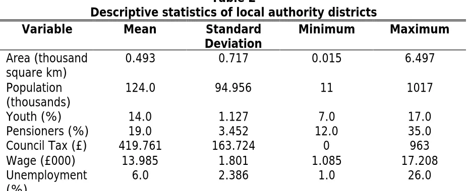
is available at LAD level on an annual basis7. Table 2 shows that they vary a
good deal across a number of dimensions such as population, leading to very
different degrees of penetration by our burger chains.
TABLE 2 HERE
2. Outlet locations
As we are interested in within market location, we calculated the distances
between outlets in our chosen markets. Using the facility on
http://www.streetmap.co.uk/ for converting postcodes to Ordnance Survey
grid co-ordinates, each was mapped to a co-ordinate8 and the Euclidean
distance between outlets calculated. We chose markets fulfilling the following
three criteria into our sample:
a. Both key players (McD and BK) are in the market at the end of our
period (end 1995).
5 The source of these last observations is inspection of the set of agreements registered with the Office of Fair Trading under the provisions of the Restrictive Trades Practices Act 1976 and subsequent legislation. Files numbered 6193, 6194, 15127 and 15678 contain examples.
6
All McD data was received from the company itself. For BK, we received the addresses of all their outlets as of end of 1995, and for a proportion, the opening dates. For the rest, we collected the opening dates from a variety of sources. For details, see Toivanen and Waterson (2003) data appendix.
7
These data largely come from Regional Trends or its sources; see again the Data Appendix to Toivanen and Waterson (2003).
8
b. We can date order which player was first into the market, and
determine the ordering of outlets up to the point at which the other
player entered.
c. There are at least three outlets associated with these players in
total.
From the set of 57 markets fitting these criteria, we stopped recording outlet
details regarding location (i.e. their postcode) once the second player had
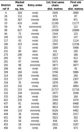
entered for the first time. Our set of districts is divided into two subsets. In
the first, consisting of the first 34 observations listed in Table 3, there are
three or more outlets (up to 6), of which only the most recent is the outlet of
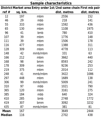
a different firm than all previous entries. In the second set, the final 23
observations, there are three outlets, with the chronological order of outlet
openings by firms A and B being A, B, A, or A, B, B.9 We use different
sub-samples of these data. Some key distance and firm statistics are shown in
Table 3. By comparison with Table 2, we note that on average, the included
districts are around 1/3 the area of the average district. Large, typically rural,
LADs mostly have few or no fast food outlets.
TABLE 3 HERE
It is noteworthy that there is a very significant difference in Table 3 between
the median distance between same-firm outlets and different-firm outlets.
3. Consumer behavior
If customers largely patronized the outlets of different firms, close spatial
location of McD and BK outlets would not be problematic from the viewpoint
9
of avoiding head to head competition. In fact, most people who buy burgers
visit both brands of outlet. A report by a market research company, Mintel
(1998) details information that allows us to calculate lower bounds for the
overlap between McD and BK by reporting what percentage of their sample i)
has visited any hamburger restaurant in the last three months, ii) McD, iii) BK.
By assuming that all those that visited a hamburger restaurant but did not
visit McD did visit BK, we can calculate that over all customer groups, at
minimum 73% of those consumers in the Mintel sample that visited a BK
outlet also visited a McD outlet. For different age groups, the figure varies
between 87% for 20-24 year olds and zero for those over 65. Calculating the
same statistic for Kentucky Fried Chicken (KFC) and BK, and setting a lower
bound of zero for the measure, we find that 0.6% of BK customers also
patronized a KFC during the three month period. This information not only
confirms the probably common prior that McD and BK are closer in product
space than BK and KFC, but also that McD and BK are close in product space.
Recall that the Mintel figures do not condition on distance, and therefore
these lower bounds already include the differentiating effect of distance. The
amount of product differentiation due to product quality is therefore even less
than these figures suggest.
IV TESTS
1. Pre-emption
Our first test is designed to discriminate between the pre-emption explanation
on the one hand, and product differentiation or learning on the other hand.
distance between the outlet of the following firm and any of the leader’s
outlets is greater or less than the distance between any of the leaders’
outlets. The Null is that there is no difference on average (i.e. that physical
location does not matter). Hence, under the Null, if the entry pattern is A, A,
B, the probability of the distance between B and one of the A’s being less
than the distance between the two A’s is 2/3. Similarly, if the pattern is A, A,
A, A, A, B, then the equivalent probability is only 1/3 (5 ways out of 15). Our
test uses a series of simulations to take into account that the probability
under the Null varies across observations.10 The alternative hypothesis of
pre-emption predicts that the follower outlet is further away from leader outlets
than the leader outlets are from each other, on average.11
For each observation in the sample, a simulation round involved a
random draw of a zero-one variable, where the indicator function takes the
value
1 iff mindist (A, B) < mindist (A, A’), for all A, A’
for a market with n “A” outlets and one “B” outlet and the probability of this
happening comes from the above calculations based on actual market
structures. We then weight these draws by the relative frequency of the
different market structures that we observe, and calculate the distribution of
the sum of “1” answers we have generated, which is a sufficient statistic for
the test. The 99th percentile of that generated distribution, 28, is compared
10
We are very grateful to Michael Pitt for his work on the details of this approach including providing the coding which enabled this test. We took a total of 40,000 simulations.
11
to what we observe in the data. This figure, 29, easily allows us to reject the
Null at better than 1% level. This is strong evidence against the pre-emption
story.
2. Product differentiation
Unlike learning, product differentiation affects the distances between any pair
of outlets. We therefore proceed under the implicit assumption that all
locations are identical, and look at markets with two outlets of one firm, and
one of the other. In this second subset of Table 3, with the form A1, B1, A2, or
A1, B1, B2, (or in four cases, a tie between A1, B1, B2 and A1, A2, B1) we test
whether the distance between the first outlet of the follower (B1) and the
initial leader outlet (A1) is less than the distance between the other pairs,
follower and third outlet and initial outlet and third outlet. Under the Null,
where fascia is irrelevant, the probability of this is 1/3. Assuming nationally
set prices (see footnote 3 above), if product differentiation is of some
importance, we expect a greater distance between the two outlets of the
same firm than between either of the other pairs, as two outlets of the same
firm produce identical products, whereas there is some – even if only a
limited amount of – product differentiation in the quality dimension between
the two rivals. Under the learning alternative we expect the least distance
between the outlets B1 and A1. 12
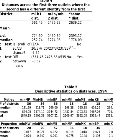
Twenty of the second set of 23 districts, listed in Table 4, across which
this test can be performed, satisfy the alternative hypothesis that is consistent
12
with learning. With a t-value of -7.64, this allows us to reject the Null in favor
of the one-sided (learning) alternative at better than 1% level. We can
alternatively test the difference between mean distances across the three
pairs. As seen in Table 4, there are large numerical differences between
these mean values. Again, the alternative consistent with learning is
accepted over the Null and the product differentiation alternative, with the
t-value related to the lesser difference being -3.57 and the difference between
the other two mean distances being insignificant.
TABLE 4 HERE
Our second test of product differentiation involves looking at the
distances between McD and BK, McD and KFC, and BK and KFC, and similarly
between the hamburger firms and Pizza Hut. The common prior would
probably be that the two hamburger firms are closer together in product
space than either is to KFC or Pizza Hut. If this is so, then we would expect
that KFC and Pizza Hut locate closer to the hamburger firms than these to
each other. Here we do not have data on opening date, simply data on
presence as of 1994. These come from the source Retail Directory of the UK.
This provides a street-by-street listing of retail outlets in most major UK town
centres, from which we extracted information on the additional chains of
interest. Therefore, in this final sample, we restrict outlets under
consideration to those that appear in the town centre.13 In order to make the
13
tests meaningful, we restrict our sample to those town centres where three or
four of the players appear.
As Table 5 shows, this distance data is noisy. A series of comparisons
are available. In the upper panel, these are performed using absolute
distances within matched sub-samples. In the lower panel, we bring distance
to a common base, so we analyze relative distances within maximally sized
sub-samples. In some ways, the median provides the best method of
comparison in this table, since outliers where the nearest outlets are some
kilometers apart affect all the means. Looking first at the three-way
comparison between McD, BK and Pizza Hut, we might expect under product
differentiation that the MB distance would be greater than the other two.
However, it is not. By contrast, the three-way comparison involving KFC does
provide some support for the product differentiation hypothesis. Yet, turning
to the comparisons involving Wimpy, no support is offered, since the MB
distance is smallest.
Now turning to the lower panel, the values listed are taken as a
proportion of the “diameter” of the LAD, assuming it approximates a circle.
Thus for example, the median distance between McD and Wimpy outlets
across 20 cases is less than 2% of the diameter of those respective districts.
The main feature coming out of this comparison is that the median
proportions are all small, save that between successive McD outlets, which is
significantly larger.
TABLE 5 HERE
All the above tests produced evidence that BK locates closer to the first
McD outlet than we would expect if pre-emption behavior, product
differentiation or pure chance explained the location patterns. Our suggestion
is that this pattern is due to learning. Alternatively, however, it could be that
the first McD outlet is located in a particularly profitable location, and BK
therefore places its (first) outlet close to the first McD. For this to be true, one
has to provide an explanation as to why the location of the first McD would
consistently be better than that of subsequent McD outlets. One possibility is
the following: assume that demand for fast food (hamburgers) in the UK ever
since the mid-70s, has increased at a constant rate both between and within
markets. Assume also that within market differences in demand are known.
Assume further that even a firm like McD faces constraints as to how many
outlets per period it can open, or alternatively, that the costs of opening an
outlet in a given period are convex in the number of outlets opened in that
period. What would be an optimal entry strategy in such circumstances?
According to this story, McD could already in 1974 when it entered the
UK rank all the possible outlet locations in terms of profitability. It would
however not be optimal to enter all locations right away, as this would
increase costs of entry compared to the alternative of opening in some
locations in the following year(s). It would be optimal to open in the best
locations first. If this is the strategy McD has followed, then the first location
in each market is the most profitable location in that market. Our above
reported findings would then simply provide evidence that BK, too, is able to
the first McD outlet. No inter-firm learning takes place. We test this story
against learning in two ways.
Our first test of learning involves a subset of the data used above. In
the product differentiation test, we looked at markets with three outlets. It
turns out that 16 of them have the entry time ordering mbm. By chance,
there are also 16 cases in our data that start mmm. This suggests a
comparison between the sets of distances in each case. In other words, the
mmm cases might serve as a useful point of reference from which to analyse
the mbm ones. Especially, it allows us for the first time to tackle the issue of
location heterogeneity. If it is true that the first McD is located in the most
profitable location within a market, then we would expect the second McD
also to be located ‘close’ to the first one (close meaning closer than the third
is to the first). Table 6 sets out the relevant means and standard deviations
for these two samples. As is fairly evident from the raw means, there is no
significant difference between any of the mean distances between outlets in
the mmm cases, providing evidence against the first outlet’s location being
better than the others. However, there is a significant difference between the
m1b and the other two distances in the mbm cases, with a t-value of over 4.
This provides evidence for learning against product differentiation. It is also
interesting that the m2b distance is not significantly different from the m1m2
distance.
TABLE 6 HERE
The theoretical justification for our second test of learning comes from
draws being positive (higher than the prior) on average, the posterior of an
experiment with a larger number of draws is larger (on average) than that of
an experiment with a smaller number of draws.14 Further, this difference is
growing in the difference in the number of draws. In our data, the inability of
BK to exploit information prior to 1990 gave it a chance to sample from
different distributions, i.e., to observe the profitability of first McD outlets in
different markets. The number of draws available to BK varied over the
markets depending on when McD had opened the first outlet, giving us
observable variation in this metric. Also, the fact that BK tends to locate close
to the first McD is evidence for the draws (signals of profitability of the
location of the first McD outlet) being on average higher than the prior.
Our hypothesis is thus an implication of Bayesian decision making: the
larger the number of draws (the longer the first McD has been in existence
prior to 1990), ceteris paribus, the higher the mean posterior, and therefore,
the more likely it is that BK locates close to the first McD outlet.
Our second set of tests exploits an implication of the above story of
how the profitability of the locations of first McD outlets varies over markets,
providing us with a way of controlling for differences in the profitability of the
first McD outlets. If McD behaves as outlined above, then the ranking of McD
outlets is an (exact, but ordinal) measure of the relative profitability of McD
outlets. Further, if BK has used time prior to 1990 to observe the profitability
of different (first in the market) McD outlets, the time a McD outlet has
14
existed prior to 1990 is a measure of the number of draws BK has been able
to sample for a given McD outlet. We therefore take all markets where McD
has at least two outlets by the time of BK entry, and estimate the following
regression:
(1) distm1,b,i = Xi'α+β1timem1,i +β2rankm1,i +εi.
In (1), the dependent variable is the distance (in meters) between the first
McD outlet and the BK outlet in market i, X is a vector of market
characteristics that controls for observed differences between markets, time is
the time prior to 1990 that the first McD outlet has been in existence in
market i, and rank is a measure of the rank of the first McD outlet in market
i.15 If our story is correct, time should be significantly negative in (1),
controlling for rank.
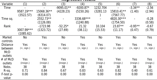
TABLE 7 HERE
We have performed a large number of estimations of (1) using
different distance, time and rank variables. We compile the evidence on the
relationship between these variables into Table 7, but suppress the results on
the control vector.16 It is clear from the reported results that despite the small
sample size, we find a consistent, most of the time statistically significant,
negative relationship between the distance at which BK locates its first outlet
from the first McD outlet and the time that the first McD outlet has been in
15
Although these measures are naturally highly correlated, the correlation is not perfect due to the large number of outlets opened each year by McD in the 1980s.
16
the market prior to 1990.17 The rank of the first outlet almost never obtains a
significant coefficient, supporting the earlier finding with the 16+16 matched
markets above. These results give further evidence in support of the learning
story.
V CONCLUSION
Although the evidence provided in this paper is of only two firms in one
national market, the flavor is clear: BK consistently locates closer to the first
McD outlet than we would expect if pre-emption, product differentiation, or
pure chance (such as local planning) were driving the location decisions. We
also find that the distance between the first McD outlet and the BK outlet is
negatively affected by the time the first McD outlet has been in the market,
conditional on the rank of the McD outlet. All this suggests that in making its
location decisions, BK learns from (the first) McD, and that this effect
overwhelms other effects on location.
The implication from an industrial organization point of view is that
notwithstanding the importance of (strategic) competition in oligopolistic
markets, inter-firm (knowledge) spillovers may be of overriding importance
even for firms that have invested a great deal into solving the problems
relating to optimal product positioning in the markets they serve. We know
they are important in R&D intensive industries, but to find they are important
in fast food retailing is rather more novel.
17
The implication from a public policy point of view is a negative one.
The UK is subject to significant planning laws constraining the opening of
certain types of retail outlet. In the case of fast food, an existing site must by
“A3” classified in order to be suitable. In the case of a new site, in order to
get a designation, the retail chain will need to assure the local planning
authority, acting for residents, that a significant nuisance such as smell or
traffic congestion will not ensue. It has been argued in other retail contexts,
in particular supermarkets (Competition Commission, 2000) that planning law
constrains the growth of competition, so enhancing the existing market power
of incumbents (see also McKinsey, 1988). However in the present context,
we found no evidence for the pre-emption view. Thus there is no evidence,
in the context of small fast food outlets, that the growth of competition is
Table 1:
Key dates in the UK history of burger retailing
Date Event
1960s Wimpy brand established as offshoot of J Lyons
1970s Wimpy established limited counter service concept
1974 McDonalds opens first store
1977 Wimpy chain bought by United Biscuits
1983 McDonalds exceeds 100 outlets
1986 McDonalds exceeds 200 outlets
McDonalds starts to franchise outlets 1988/89
1989 Burger King brand (at this time small) bought by Grand Met Grand Met buys Wimpy from United Biscuits
1990 Burger King has 60 outlets
Grand Mets burger operations separated into table and counter service Counter Service operations mostly re-badged as Burger King
Wimpy International (with 220 table-service outlets) formed by management buy-out from Grand Met
Grand Met insists on 3 year agreement preventing Wimpy opening counter service or drive in outlets
1993 June: Grand Met/ Wimpy agreement expires
McDonalds has around 500 outlets
1994 Wimpy has 240 outlets, all eat-in
end 1995 Burger King has approx. 300 outlets McDonalds has over 600 outlets
May 1996 Wimpy has 272 outlets
McDonalds and Burger King each opening around 70 restaurants per year
Table 2
Descriptive statistics of local authority districts Variable Mean Standard
Deviation Minimum Maximum
Area (thousand
square km) 0.493 0.717 0.015 6.497
Population
(thousands) 124.0 94.956 11 1017
Youth (%) 14.0 1.127 7.0 17.0
Pensioners (%) 19.0 3.452 12.0 35.0
Council Tax (£) 419.761 163.724 0 963
Wage (£000) 13.985 1.801 1.085 17.208
Unemployment
Table 3
Sample characteristics
District Market area Entry order 1st/2nd same chain First mb pair
ref # sq. km. dist. metres dist. metres
4 204 mmb 2445 2690
26 112 mmb 475 87
50 367 mmmb 8934 971
53 410 mmb 11165 11177 59 78 mmmmmb 2571 122 89 637 mmb 14358 20889
94 75 mmmb 1544 125
100 333 mmb 1917 147
117 43 mmb 1252 1114
180 315 mmb 3597 11536
181 32 mmb 1609 5468
231 80 bbm 422 185
275 290 mmb 3617 180
283 93 mmb 1325 612
291 97 mmmb 5471 680
292 98 mmmmb 3877 3877
296 69 mmb 1453 45
309 160 mmb 5790 5886 314 199 mmmb 9541 260 315 137 mmb 2300 2307
316 35 mmmb 1876 299
323 142 mmb 2655 4893 331 153 mmmmmb 21717 21716 333 159 mmmb 3477 3548
370 246 mmb 5304 160
422 235 mmb 3293 3374 437 81 mmmb 3852 6468 438 48 mmmb 4614 5419 444 110 mmmmb 6326 4482 448 38 mmmb 3603 3317
451 38 mmmb 3021 302
453 56 mmmb 656 420
455 29 mmmmb 2931 3187
Table 3 continued Sample characteristics
District Market areaEntry order1st/2nd same chainFirst mb pair
ref # sq. km. dist. metres dist. metres
12 197 mbm 2556 152
46 29 mbb 218 141
55 333 mbm 1592 436
65 130 mbm 1108 1975
96 41 bmb 780 410
107 39 mbm 1776 148
111 39 mbm 1506 178
116 477 mbm 1388 311
128 309 mbm 4778 113
148 42 mmb/mbm 331 63
166 212 mbm 3662 440
168 98 bmm 8593 242
178 309 mbm 9236 253
219 375 mbm 2014 112
248 41 mmb/mbm 3422 1086
297 448 mbm 1689 138
306 99 mmb/mbm 5009 241
310 97 mbb 1021 790
365 120 mbm 3161 275
385 184 mbb 640 324
410 285 bmb 2748 1772 419 307 bmm 3092 3232 435 87 mmb/mbm 381 81
Mean 167 3649 2444
Table 4
Distances across the first three outlets where the second has a different identity from the first District m1b1
dist. m2b/mb2 dist. “same” dist.
Mean
561.45 2476.88 2639.22
s.d. 774.50 2450.80 2393.17
median 252.74 1774.08 1776.09
t test
1 Is prob of 20/23 chance?
(1/3-20/3)/((20/23*3/23)/23)0.5=
-7.64
No
t test
2 Diff between
means
(561.45-2476.88)/535.9=
-3.57 Yes
Table 5
Descriptive statistics on distances, 1994
Metres minMP MinMB minBP minMK minMB min KB minMW minBW min MB
# of districts 36 36 36 18 18 18 20 20 20
median 181.69 218.71 299.00 198.28 525.88 405.29 234.19 305.90 181.55
mean 824.95 1174.10 2744.72 1432.84 1703.73 2467.08 705.80 2900.58 1511.12
sd 1849.15 3505.38 5307.21 2209.97 2852.08 3555.44 1392.98 5539.15 3032.42
Proportion minMW minBW minMB minMP minMK minBP min KB min MM
# of districts 20 20 57 36 18 36 18 51
median 0.017 0.021 0.022 0.014 0.018 0.024 0.034 0.197
mean 0.074 0.242 0.091 0.075 0.148 0.195 0.183 0.225
Table 6
Comparisons across successive outlet differences
Outlets 1 and 2 2 and 3 1 and 3 between means Differences
mmm mean 5250.69 4576.91 5284.55 All insignificant
sd 5021.30 2893.19 4127.67
mbm mean 375.187 2666.46 2725.63 t=-4.08
sd 492.34 2190.24 2225.34 at least
Table 7
Regression results
Variable (1) (2) (3) (4) (5) (6) (7) (8) Time
-9587.19*** (3522.57) -15068.36** (6314.07) -9095.01**
(4228.23) -9200.87* (5150.26) 1232.704 (3281.13 )
-15810.41** (7567.77)
-3.34**
(1.40) (2.94) -2.56
Time sq. - 2552.73**
(1126.08) - 3336.68*** (1240.88) - 4820.30*** (1754.50) - (0.58) -0.28 Rank
-3007.99*** (1085.62)
-1723.98
(1323.72) -52.25* (27.69) (38.11) 21.32 (15.53) 10.104 23.87** (11.17) -0.95** (0.47) (0.79) -0.67
Market
controls No Yes No Yes No Yes No Yes Distance between McD outlets Yes (+, sign.) Yes
(+, sign.) (+, sign.) Yes (+, sign.) Yes (+, sign.) Yes (+, sign.) Yes (+, sign.) Yes (+, sign.) Yes
# of McD outlets
Yes (insign.)
Yes
(insign.) (insign.) Yes (insign.) Yes (insign.) Yes (insign.) Yes (insign.) Yes (insign.) Yes
Nobs. 38 38 38 38 38 38 38 38
R-sq. 0.71 0.84 0.67 0.83 0.63 0.82 0.40 0.61 F-test
p-value 0.00 0.00 0.00 0.00 0.00 0.00 0.00 0.00 Notes:
Dependent variable is distance between first McD outlet and the BK outlet (in meters) in Columns (1)-(6), and its natural logarithm in (7)-(8).
Reported numbers are coefficient and (standard error). Standard errors are robust to heteroskedasticity of unknown form.
***, **, and *, and denote significance at 1, 5 and 10 per cent levels.
The measure of signal (Time) is the natural log of time of the first McD outlet in the market prior to 1990 in Columns (1) and (2) and (7) and (8), and the same in linear form in Columns (3) and (4). In Columns (5) and (6) the measure is the natural logarithm between the time of entry of the first McD and BK outlets.
In Columns (1)-(2) and (7)-(8) the measure of the rank of the first McD is a categorical variable increasing in value by 1 after each additional 50 outlets. In Columns (3)-(6) the measure of rank is the actual rank of the first McD outlet.
Market controls include the population and the geographic area of the market, the proportion of under-16 and over 65-year olds, an indicator for markets in London, and the number of McD (BK) outlets in neighboring districts as of beginning of the year of BK entry. Of these, youth and pension coefficients were usually significant and positive, population’s negative and significant. Others’ coefficients were never significant.
REFERENCES
Baum, J.A.C., Li, S.X., and Usher, J.M., 2000, "Making the Next Move: How Experiental and
Vicarious Learning Shape the Locations of Firms Acquisitions", Administrative Science
Quarterly, 45, pp.766-801.
Berry, S.T., 1992, "Estimation of a Model of Entry in the Airline Industry”, Econometrica, 60,
pp. 889-917.
Bresnahan, T.F., and Reiss, P.C., 1989, “Do Entry Conditions Vary Across Markets?”,
Brookings Papers on Economic Activity, 3, 883-871.
Bresnahan, T.F., and Reiss, P.C., 1990a, “Entry in Monopoly Markets”, Review of Economic
Studies, 57, 531-553.
Bresnahan, T.F., and Reiss, P.C., 1990b, “Empirical Models of Discrete Games”, Journal of
Econometrics, 48, 1-2, 57-81.
Bresnahan, T.F. and Reiss, P.C., 1991, “Entry and Competition in Concentrated Markets”,
Journal of Political Economy, 99, 977-1009.
Bresnahan, T.F., and Reiss, P.C., 1994, “Measuring the Importance of Sunk Costs”, Annales
d’Economie et de Statistique, 0, 181-217.
Caplin, A. and Leahy, J., 1998, "Miracle on Sixth Avenue: Information externalities and
search," Economic Journal, 60-74.
Competition Commission, 2000, Supermarkets: A report on the supply of groceries from
multiple stores in the United Kingdom, Cm 4842, HMSO, London.
Davis, P., 2002, The Effect of Local Competition on Retail Prices: The US Motion Picture
Exhibition Market, mimeo, LSE.
DeGroot, M.H., 1970, Optimal Statistical Decisions, New York, McGraw-Hill.
Eaton, B.C. and Lipsey, R.G., 1979, The theory of market pre-emption: The persistence of
excess capacity and monopoly in growing markets, Economica, 46, 149-158.
Ellison, G., and Glaeser, E., 1997, Geographic Concentration in U.S. Manufacturing Industries:
A Dartboard Approach, Journal of Political Economy, 105, 5, 889-927.
Ellison, G., and Gleaser, 1999, The Geographic Concentration of Industry::Does Natural
Joseph, A., 2003, Spatial competition between franchisees, Mimeo, Tinbergen Institute.
November.
Mazzeo, M., 2002, “Product Choice and Oligopoly Market Structure”, RAND Journal of
Economics, 33, 221-242.
McKinsey, 1988, Driving productivity and growth in the UK economy, McKinsey Inc, London.
Mintel, 1998, Burger and chicken restaurants- UK- April 1998, Mintel International Group.
Petrin, A., 2002, Quantifying the Benefits of New Products: The Case of the Minivan, Journal
of Political Economy , 110, 705-729.
Seim., K, 2002, An Empirical Model of Firm Entry with Endogenous Product-Type Choices,
mimeo, GSB Stanford.
Toivanen, O., and Waterson, M., 2003, Market structure and Entry: Where’s the Beef?
Mimeo, University of Warwick.
Trajtenberg, M., 1989, The Welfare Analysis of Product Innovations, with an Application to
Computed Tomography Scanners, Journal of Political Economy, 97, 444-479.
West, D.S., 1981, Testing for market preemption using sequential location data, Bell Journal