Supervised sampling for clustering large data sets

(1)

University of Warwick institutional repository: http://go.warwick.ac.uk/wrap

This paper is made available online in accordance with

publisher policies. Please scroll down to view the document

itself. Please refer to the repository record for this item and our

policy information available from the repository home page for

further information.

To see the final version of this paper please visit the publisher’s website

.

Access to the published version may require a subscription.

Author(s): I Kosmidis and D Karlis

Article Title: Supervised sampling for clustering large data sets

Year of publication: 2010

http://www2.warwick.ac.uk/fac/sci/statistics/crism/research/2010/paper

10-10

(2)

Supervised sampling for clustering large data sets

Ioannis Kosmidis

CRiSM and Department of Statistics, University of Warwick Coventry, CV4 9EL, UK

[email protected]

Dimitris Karlis

Department of Statistics, Athens University of Economics and Business 76 Patision Str, Athens, 10434, Greece

[email protected]

June 12, 2010

Abstract

The problem of clustering large data sets has attracted a lot of current research. The approaches taken are mainly based either on the more efficient implementation or modification of existing methods or/and on the construction of clusters from a small sub-sample of the data and then the assignment of all observations in those clusters. The current paper focuses on the latter direction. An alternative supervised procedure to create the clusters is proposed. For learning the clusters, the procedure is using subsets of the data which are still constructed via sub-sampling but within partitions of the observation space. The general applicability of the approach is discussed together with tuning the parameters that it depends on to increase its ability. The procedure is applied to clustering the navigation patterns in the msnbc.com database.

Keywords: sub-sample; partition; hard clustering; clustering click-stream data

1 Introduction

In recent days, mainly due to the automatization in data collection procedures, the size of the data sets has dramatically increased posing challenges to their statistical treatment. Typical examples of such data sets are MRI pictures, transaction data from super markets and web-usage data, where millions of observations are available. In this respect, clustering methods can be very helpful to summarize these large data sets into few sets of equivalent, in some appropriate sense, observations or to identify useful patterns. However, most of the classical clustering methods (such as k-means, hierarchical clustering methods and model-based approaches and their variants) have been designed to cope with relatively small data sets and their scaling to huge data sets is not obvious or efficient.

(3)

and computer resources (see Bradley et al., 1998a,b; Farnstrom et al., 2000). Some other ideas applicable in hierarchical clustering can be seen in Tantrum et al. (2004) and Vijaya et al. (2004). See, also Fraley et al. (2005) for an incremental algorithm.

Another class of approaches to clustering large data sets is to construct the clusters based on a small random sub-sample of the data. This approach dates back to Kaufman and Rousseeuw (1986) (CLARA algorithm). The key idea is to run the selected clustering algorithm to several random sub-samples of the data and then decide, according to some optimality criterion, which of the derived cluster configurations to use for the classification of the rest of the data. Due to their simplicity such approaches can be used to provide starting points to more sophisticated clustering methods (as is done for example in Steiner and Hudec, 2007, in order to construct a large numbers of prototype clusters which are subsequently combined into fewer ones using a more sophisticated model-based approach). However, random sub-sampling in combination with hard clustering algorithms can return unstable results (see, for example Posse, 2001; Wehrens et al., 2004), especially when small groups are present in the data. A reason for this is that observations in the small groups possibly present in the data may not be selected via random sub-sampling.

To overcome such drawbacks, in the current paper, a model-free, supervised way of selecting subsets of the data is proposed, which aims to be robust to the deficiencies of random sub-sampling for clustering applications. The suggested procedure uses random sub-sampling and some k-medoids clustering method but within partitions of the obser-vation space. In this way, small groups can be slightly over-represented in the resulting subsets and thus usual clustering algorithms can reveal their existence. Furthermore, the proposed procedure depends on several user-defined parameters and offers a way to take a finite number of subsets from the data and decide which is the best to use according to some optimality criterion. Finally the procedure applies to diverse types of data and clustering algorithms.

The remaining of the paper proceeds as follows: Section 2 describes the main idea and the contribution of the paper. In Section 3, the proposed procedure is applied on a simulated data set and Section 4 is concerned with the currently fashionable problem

of web-clustering, where huge data sets are involved. Specifically, users are clustered

according to their browsing behavior. Finally, a discussion and concluding remarks can be found in Section 5.

2 The proposed procedure

2.1 Motivation

When clustering large data sets, a common approach is to take a much smaller subset of the observations and use it for the necessary inferences, avoiding, in this way, the computa-tional issues that arise when using all the observations in the data set. The most common approach is random sub-sampling (for example, as in the CLARA procedure). However, in this way the observations in small groups have correspondingly small probability of being selected, which might result in failure of detecting those small groups.

(4)

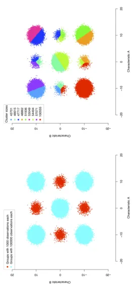
construction of 9 clusters, taking, for robustness, 400 sub-samples of size 1000 each. The resulting clustering is shown in the right plot of Figure 1. Clearly, despite the simplicity of the structure of the data and the large number of random sub-samples used, CLARA fails to correctly detect the true groups, breaking up the large groups and fusing the small groups into large clusters.

A different approach which would allow small groups to be slightly over-represented in the subsets could enable the clustering algorithms to construct corresponding small clusters. This can be done by partitioning the observation space and then retrieving ran-dom sub-samples within the partitions, because then the probability that an observation is selected in any partition may differ between observations.

2.2 Data-dependent partitions of the observation space

Let x1, . . . , xN be N observations belonging to an observation space Ω and define an

appropriate, positive-valued measure d(., .) for measuring the dissimilarity between any

two observations. Furthermore, let ˆµbe an element of Ω which, in some appropriate sense,

is located centrally relative to the observations x1, . . . , xN. For example, in Euclidean

spaces, ˆµ may be set as the mean vector ofx1, . . . , xN.

Denote by x(1), . . . , x(N) the observations sorted in increasing distance from ˆµ and

without loss of generality, suppose that the observation space is Euclidean. Consider the creation ofh−1 concentric hyper-spheres F1, . . . , Fh−1 with center ˆµand radiir1≤...≤

rh−1, respectively, which are defined by the data as

ri = max j∈{1,...,i[N/h]}d

x(j),µˆ (i= 1, . . . , h−1),

where [N/h] isN/h rounded to the closest integer. Furthermore, setrh = +∞.

Using the above construction, the observation space may be partitioned in partitions

I1, . . . , Ih, where

I1 = F1

Ii = Fi∩Fic−1 (i= 2, . . . , h),

withFh = Ω.

Such a partitioning scheme depends exclusively on the observed data and results in

partitions with [N/h] observations each, where the last partition may contain more or

fewer observations than the others depending on the value ofN/h.

In this way, letting r0 = 0, the observations xj with j ∈ D, D ⊂ {1, . . . , N} are

equivalent if and only ifri−1≤d(xj,µˆ)< ri for allj ∈D, for somei= 1, . . . , h.

The above equivalence relations motivate the treatment of each partition

indepen-dently. Random sub-sampling without replacement can be used to obtains sub-samples

of sizenfrom each partition and a k-medoids clustering algorithm (for example the PAM

algorithm in Kaufman and Rousseeuw (1990)) can be applied to each sub-sample to obtain

ccentroids. The resultant centroids may be thought as summarizing the information of the

(5)

Figure

1:

Left:

Sim

ulated

data

consisting

of

504000

ob

serv

ations

of

tw

o

real-v

alued

characteristics

A

and

B.

The

data

form

9

w

ell-separated

groups

where

the

red

gr

oups

con

tain

1000

observ

ations

eac

h

and

the

cy

an

groups

100000

obse

rv

ations

eac

h.

Righ

t:

The

resulting

clustering

from

the

application

of

CLARA

with

400

sub-samples

of

size

1000

eac

[image:5.595.196.459.133.733.2]

(6)

2.3 Specification of the parameters h, s, n and c

The above construction requires the specification of the parametersh,s,nandc. Ifh= 1,

the procedure is equivalent to obtaining all the centroids that result from the application

of k-medoids withccentroids on each one ofsrandom sub-samples with sizen, where the

sub-samples are taken from all the available data points. This, in turn, is similar — but not the same — to collecting the resulting centroids in the iterations of CLARA and using them as a representative subset of the data. A systematic way of specifying the values of those parameters may be constructed by noting that the number of elements sampled in the aforementioned elementary setting can serve as the reference amount of information for the definition of possible partitioning schemes.

Suppose that the resulting subsets are used for clustering the data inm≤M clusters.

First, note that the size of the resultant subset of observations ishsc. The total number

of elements that are sampled during the procedure isk=hsn. Thus, specifyingk we can

enumerate all possible combinations of positive integersh,s,nand c, for which k=hsn

is solved under the natural constraints

hsc ≥ M , (1)

c ≥ 1,

n ≥ c ,

[N/h] ≥ n ,

h > 1,

s ≥ 1.

The first constraint ensures that the maximum number of clusters to be constructed using the subset is smaller than the size of the subset.

Clearly, the solution set after definingk is either empty or finite, because h, s, nand

care all positive integers. Thus, fixingkto an appropriate value, the procedure described

in the previous section can be applied for all possible quadruplets (h, s, n, c) for which

k=hsnis solved subject to the constraints (1), and the subset that gives the best results

for the original data can be selected according to some application dependent optimality

criterion. As is done in later sections,ccan also be fixed at some integer value instead of

allowing it to vary freely. In this way, the number of settings that need to be considered is greatly reduced.

2.4 Steps of the suggested procedure

After having chosen ˆµ, the procedure involves the following steps:

A. Initialization

A.1 Calculate di=d(xi,µˆ),i= 1, . . . , N.

A.2 Sort di,i= 1, . . . , N, in increasing order.

A.3 Order the observations according to the ordering ofdis and obtain the ordered sample

(7)

B. Main iterations

For every (h, s, n, c) that solvesk=hsnunder the constraints (1), the following steps are

repeatedt times.

B.1 Constructh observation sets

G1 = {x(1), . . . , x([N/h])},

.. .

Gh−1 = {x((h−2)[N/h]+1), . . . , x((h−1)[N/h])},

Gh = {x((h−1)[N/h]+1), . . . , x(N)}.

B.2 For j= 1 to h

B.2.1 Obtain srandom sub-samples of size nfrom Gj.

B.2.2 Apply a k-medoids clustering algorithm with ccentroids to each sub-sample.

B.3 Apply a clustering algorithm on the subset of the data consisting of all the centroids that were obtained in the previous steps.

B.4 Classify all the observations in the data set in the resultant clusters.

B.5 Calculate some appropriate optimality criterion for the clustering on all observations of the data set.

Note that step B.5 can be expensive for extremely large data sets. In such cases, steps B.4 and B.5 can be omitted, calculating the optimality criterion merely for the clustering of the subset that results in step B.3.

2.5 Computational considerations

For any specific choice of (h, s, n, c), the total number of calculations required for the

application of the proposed procedure is O(N) +r(n, s, h, c). The O(N) term reflects

the effort required for calculating and sorting d(xi,µˆ) (i = 1, . . . , n) (which only needs

to be done once for all available quadruplets (h, s, n, c)) and for the classification of the

observations in step B.4 of the procedure. The term r(n, h, s, c) is appearing due to the

additional calculations required for the application of a k-medoids clustering algorithm to

each of the ssub-samples of size n. Nevertheless, the extra effort r(n, h, s, c) is not very

large given that the clustering algorithm is applied to a small subset of the observations contained in a partition.

3 Application to simulated data

To demonstrate its benefits and functionality, the proposed procedure is applied to the example of Section 2.1. Interest is in detecting well-separated small groups, and thus the optimality criterion for the selection of the best clustering is chosen to be the maximum average silhouette width. The average silhouette widths are calculated for the clustering

(8)

[image:8.595.103.493.151.566.2]

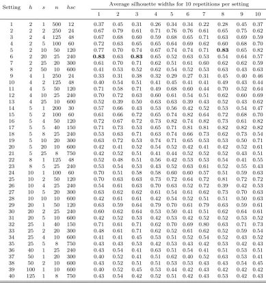
Table 1: Average silhouette widths when clustering the subsets corresponding to all

pos-sible settings of h, sand n for k = 1000, c = 6 and M = 9. The procedure is repeated

t= 10 times per setting. For each subset 9 clusters are constructed.

Setting h s n hsc Average silhouette widths for 10 repetitions per setting

1 2 3 4 5 6 7 8 9 10

1 2 1 500 12 0.37 0.45 0.31 0.26 0.34 0.34 0.22 0.28 0.45 0.37 2 2 2 250 24 0.67 0.79 0.61 0.71 0.76 0.76 0.61 0.65 0.75 0.62 3 2 4 125 48 0.67 0.68 0.60 0.59 0.68 0.65 0.71 0.63 0.69 0.59 4 2 5 100 60 0.72 0.63 0.65 0.65 0.64 0.69 0.62 0.60 0.68 0.70 5 2 10 50 120 0.77 0.70 0.74 0.67 0.74 0.74 0.71 0.83 0.65 0.82 6 2 20 25 240 0.83 0.63 0.83 0.65 0.52 0.63 0.53 0.54 0.64 0.57 7 2 25 20 300 0.61 0.70 0.71 0.62 0.51 0.61 0.60 0.62 0.62 0.59 8 2 50 10 600 0.41 0.53 0.52 0.62 0.54 0.52 0.53 0.63 0.43 0.63 9 4 1 250 24 0.33 0.31 0.38 0.32 0.29 0.27 0.31 0.45 0.40 0.46 10 4 2 125 48 0.40 0.54 0.51 0.41 0.45 0.41 0.41 0.49 0.43 0.44 11 4 5 50 120 0.71 0.58 0.71 0.49 0.68 0.60 0.44 0.70 0.52 0.64 12 4 10 25 240 0.70 0.72 0.63 0.60 0.61 0.54 0.51 0.62 0.60 0.69 13 4 25 10 600 0.52 0.39 0.50 0.63 0.63 0.39 0.43 0.52 0.43 0.62 14 5 1 200 30 0.57 0.66 0.43 0.53 0.56 0.42 0.52 0.53 0.54 0.47 15 5 2 100 60 0.61 0.66 0.72 0.65 0.74 0.82 0.64 0.72 0.68 0.70 16 5 4 50 120 0.72 0.67 0.72 0.73 0.82 0.74 0.82 0.73 0.61 0.82 17 5 5 40 150 0.71 0.73 0.53 0.65 0.71 0.81 0.81 0.82 0.82 0.82 18 5 8 25 240 0.53 0.63 0.71 0.63 0.74 0.66 0.73 0.62 0.73 0.54 19 5 10 20 300 0.63 0.72 0.53 0.74 0.71 0.65 0.53 0.53 0.50 0.71 20 5 20 10 600 0.42 0.41 0.52 0.54 0.52 0.42 0.41 0.42 0.52 0.61 21 5 25 8 750 0.42 0.52 0.51 0.41 0.44 0.52 0.52 0.52 0.43 0.51 22 8 1 125 48 0.52 0.48 0.51 0.56 0.42 0.53 0.53 0.54 0.41 0.55 23 8 5 25 240 0.53 0.54 0.53 0.43 0.52 0.63 0.61 0.52 0.55 0.43 24 10 1 100 60 0.70 0.51 0.58 0.58 0.60 0.60 0.57 0.51 0.59 0.63 25 10 2 50 120 0.70 0.63 0.63 0.73 0.72 0.64 0.72 0.81 0.72 0.72 26 10 4 25 240 0.54 0.61 0.63 0.70 0.63 0.52 0.72 0.39 0.42 0.53 27 10 5 20 300 0.63 0.62 0.62 0.61 0.54 0.61 0.62 0.73 0.70 0.63 28 10 10 10 600 0.42 0.61 0.61 0.42 0.54 0.52 0.51 0.51 0.50 0.63 29 20 1 50 120 0.63 0.59 0.64 0.79 0.70 0.61 0.79 0.63 0.59 0.61 30 20 2 25 240 0.60 0.62 0.64 0.53 0.50 0.41 0.51 0.62 0.64 0.61 31 20 5 10 600 0.42 0.52 0.53 0.42 0.53 0.42 0.52 0.52 0.53 0.52 32 25 1 40 150 0.71 0.61 0.71 0.62 0.70 0.69 0.80 0.63 0.71 0.73 33 25 2 20 300 0.48 0.61 0.71 0.62 0.52 0.61 0.62 0.52 0.59 0.54 34 25 4 10 600 0.41 0.41 0.45 0.53 0.51 0.52 0.54 0.52 0.43 0.52 35 25 5 8 750 0.43 0.43 0.53 0.42 0.53 0.43 0.42 0.53 0.42 0.43 36 40 1 25 240 0.43 0.54 0.41 0.63 0.51 0.54 0.41 0.51 0.53 0.51 37 50 1 20 300 0.40 0.52 0.41 0.51 0.62 0.40 0.52 0.63 0.53 0.41 38 50 2 10 600 0.43 0.52 0.51 0.51 0.53 0.53 0.43 0.43 0.54 0.45 39 100 1 10 600 0.40 0.52 0.45 0.53 0.44 0.42 0.43 0.42 0.42 0.42 40 125 1 8 750 0.43 0.54 0.42 0.52 0.51 0.42 0.43 0.53 0.42 0.43

observations (thus steps B.4 and B.5 are omitted). The required centrally located point ˆ

µis chosen to be the sample mean vector.

Fork= 1000 and forc= 6, Table 1 shows the possible solutions of k=hsnunder the

constraints (1) along with the size of the resultant subset of observations and the average

silhouette widths (in two significant places) int= 10 repetitions per setting. The settings

that result in the largest average silhouette width are setting 5 (h = 2, s= 10, n= 50)

in the seventh repetition and setting 6 (h = 2, s = 20, n = 25) in the first and third

repetitions, where the average silhouette width has value 0.83 (those cases are shown in

(9)

two settings is identical and is shown in Figure 2.

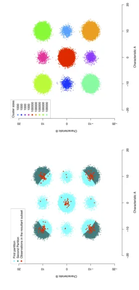
In this artificial example the assumed observation groups are fully reconstructed by merely using partitioning, random sub-sampling and a hard clustering algorithm. Fur-thermore, the total number of observations sampled for producing Table 1 and the effort required for the application of the PAM procedure, are both comparable to the corre-sponding requirements for the application of CLARA in Section 2.1.

As a final observation, note that settings 15, 16, 17 also result in average silhouette

widths greater than 0.8 and the corresponding clusterings of all the observations in the

data set are equally good.

4 A hard clustering of the msnbc.com data

4.1 Description of the data

The proposed procedure is used to obtain a clustering of the msnbc.com data set1. The

data consist of records for all the users who visitedmsnbc.com on the entire day of 28th

September 1999. For each user the ordered sequence of URL hits is recorded. Nevertheless, what is given is the category where each URL belongs to and not the URL itself. The URL categories are coded as 1: front page, 2: news, 3: tech, 4: local, 5: opinion, 6: on-air, 7: misc, 8: weather, 9: health, 10: living, 11: business, 12: sports, 13: summary, 14: bulletin board service, 15: travel, 16: msn-news, 17: msn-sports. For example, two observations in the data are

user A: 6 9 4 4 4 10 3 10 5 10 4 4 4

user B: 1 2 1 14 14 14 14 14 14 14 14 14 14 14 14 1 2 2

Thus, user A first visits a URL of category 6, then a URL of category 9, then 4, followed by another of category 4, and so on. The length of the sequences in the data varies from 1 to 14795 URL hits, which combined with the fact that there are 989818 sequences makes the construction of clusters challenging. An attempt can be found in Cadez et al. (2003) where mixtures of first-order Markov models are used to cluster these data; through an Expectation Maximization (EM) algorithm variant, the models therein are trained using a random sample of 100023 sequences and the result is evaluated using another sub-sample of 98687 sequences. The conclusion of Cadez et al. (2003) analyses was that there are 60 to 100 clusters on the data.

4.2 Clustering the msnbc.com data

In this section we attempt to group the msnbc.com data in m ≤ 20 clusters using the

proposed procedure with k = 5000 and c = 10. These parameter values result in 69

triplets (h, s, n) that solve k =hsn under the constraints (1) and we choose to use only

the 55 triplets that correspond to more than one subset per partition. The procedure is

repeated t= 10 times for each setting. We have selected to work with up to 20 clusters

mainly for illustration but also because a much larger number of clusters would have been hard to interpret and present.

The grouping of each subset in mclusters, (m= 2, . . . ,20) results by using the string

edit distance for calculating dissimilarities (see, for example, Hay et al., 2004, for a de-scription and the use of the string edit distance in the analyses of server-logs) and PAM.

1_{the data set is publicly available at}

(10)

Figure

2:

The

subset

of

observ

ations

and

corresp

on

ding

clustering

of

the

data

for

the

first

rep

etition

of

setting

[image:10.595.169.447.141.719.2]

(11)

The most dominant sequence in the data is6with 91805 occurrences (almost 9.2% of the data). Nevertheless, taking into account the nature of the string edit distance, the

“cen-trally” located observation ˆµ in the data is set to the second most dominant sequence in

the data,1(with 57552 occurrences), because the URLs of category “front page” are the

most common in the msnbc.com data. The best clustering inm clusters,m∈ {2, . . . ,20},

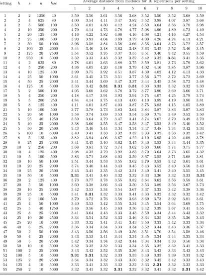
is chosen amongst at most 550 alternatives as the clustering that gives the smallest average distance from the medoids when all sequences in the data are assigned in the clusters (step B.5 of the proposed procedure). For example, in the construction of 11 clusters, Table 2

shows the average distances from medoids for the t = 10 repetitions per setting, in two

significant places. The minimum value for the average distance from medoids is 3.31 and it

is attained for several settings in Table 2. For example, for the setting 16 (h= 4,s= 125,

n= 10) that value is attained in the third repetition. All those optimal settings produce

very similar clusterings of the observations and so arbitrarily choosing one of them for

each value ofmdoes not affect the result. In this way, a list of clusterings in 2, 3,. . ., and

20 clusters is constructed.

4.3 Assessing the number of clusters

For choosing an optimal number of clusters we use the concept ofopen sequences. An open

sequence in the current context is defined as an ordered sequence of two URL categories

or more, where the same category cannot occur two times consecutively (B¨uchner et al.,

1999, used open sequences to describe navigational patterns). For example, the sequence

{2,14,14,1} is not an open sequence because the URL category 14 appears two times

consecutively. On the other hand,{2,1,14,2}is an open sequence and is contained in the

sequence for user B in Subsection 4.1, because 2, 1, 14 and 2 appear in this specific order

when we read the observed URL categories from left to right. The support of an open

sequence is defined as the number of sequences in the data containing the open sequence divided by the total number of observations in the data set. The connection between

open sequences and clusters is made via theassociation rule “If the observation contains

the open sequence then the observation belongs to cluster j”. Then, theconfidence of the

above association rule (or, equivalently, the confidence of the open sequence in clusterj)

is the number of observations in cluster j containing the open sequence divided by the

total number of observations in the data containing it. High values for the confidence of an open-sequence in a cluster suggests that users containing that open sequence are highly associated with that cluster.

For each one of the optimal clusterings, the confidences of all l open sequences that

have support greater or equal than a threshold >0, are calculated. Then the functions

P(m) = m

l(m−1) l

X

i=1

m

X

j=1

wij(1−wij),

Q(m) =− 1

llogm l

X

i=1

m

X

j=1

wijlogwij,

are evaluated at m ∈ {2, . . . ,20}, where wij is specific to each clustering in m clusters

and denotes the confidence of theith open sequence for the jth cluster (i= 1, . . . , l;j =

1, . . . , m). The dependence of wij to each clustering in m clusters is suppressed for

no-tational simplicity. By the definition of confidence, Pm

(12)

[image:12.595.94.509.180.736.2]

Table 2: Average distance from medoids when clustering the subsets corresponding to the

settings of h, s and n for k = 5000, c = 10 and M = 20. Only the settings with s > 1

are considered and the procedure is repeatedt= 10 times per setting. For each subset 11

clusters are constructed.

Setting h s n hsc Average distance from medoids for 10 repetitions per setting

1 2 3 4 5 6 7 8 9 10

(13)

[image:13.595.87.494.147.334.2]

Figure 3: The values of P(m) and Q(m) for the clusterings obtained in Subsection 4.2.

The support threshold is set to= 0.02

● _● ●

● _● ● ● ●

● ● ● ● _●

● ● ● ● ● ●

5 10 15 20

0.0

0.2

0.4

0.6

0.8

1.0

P(m) versus m

m

P

(

m

)

● ●

● ● ● ● ●

●

● ● ● _● ● _● ● ● ●

5 10 15 20

0.0

0.2

0.4

0.6

0.8

1.0

Q(m) versus m

m

Q

(

m

)

that a clustering where each open sequence has confidence 1 for some cluster and 0 for the

rest would be ideal because then thel open sequences are perfectly represented by them

clusters. In that caseP(m) =Q(m) = 0. On the other hand, the worst case scenario is

wij = 1/m (i= 1, . . . , m;j = 1, . . . , l) and hence P(m) = Q(m) = 1. Thus, given that

P(m) andQ(m) take values in the interval [0,1], preferable clusterings could be considered

the ones that correspond to small values ofP(m) andQ(m). However, depending blindly

on these criteria may return misleading results, especially for smallm, becauseP(m) and

Q(m) can take small values also when there exists a single, possibly big, cluster wherein

all open-sequences have very high confidence. Hence, some conservatism is needed when assessing the number of clusters based on these criteria.

For the msnbc.com data,is set to 0.02 and the values ofP(m) andQ(m) are calculated

for the clusterings obtained in Subsection 4.2. The result is shown in Figure 3. The

smallest value of both criteria results for m = 3 but the conservative choice of m = 6

seems to be satisfactory, because for 8 to 11 clusters the values of P(m) and Q(m) are

almost unchanged and for 12 to 20 clustersP(m) and Q(m) take bigger values.

4.4 Description of the clusters

(14)

[image:14.595.84.501.166.458.2]

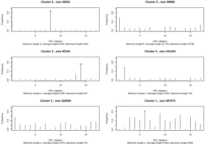
Figure 4: The frequency of appearance of each URL category in the corresponding cluster relative to its frequency in the whole data set. The size of each cluster and the minimum, average and maximum length of the sequences within each cluster are shown on the title and the subtitle of the corresponding plot.

5 10 15

0.0

0.4

0.8

URL category

Frequency

Cluster 6 , size 48291

Minimum length:3, Average length:9.829, Maximum length:1922 8

5 10 15

0.0

0.4

0.8

URL category

Frequency

5 10 15

0.0

0.4

0.8

URL category

Frequency

5 10 15

0.0

0.4

0.8

URL category

Frequency

5 10 15

0.0

0.4

0.8

URL category

Frequency

5 10 15

0.0

0.4

0.8

URL category

Frequency

on the plots. Note that, Figure 4 and Figure 5 are merely a useful visualization of the by-row and by-column relative frequencies from the cross-tabulation of clusters and URL categories.

(15)

[image:15.595.85.502.166.459.2]

Figure 5: The frequency of appearance of each URL category in the corresponding cluster relative to the number of URLs appearing in that cluster. The size of each cluster and the minimum, average and maximum length of the sequences within each cluster are shown on the title and the subtitle of the corresponding plot.

5 10 15

0.0

0.4

0.8

URL category

Frequency

5 10 15

0.0

0.4

0.8

URL category

Frequency

5 10 15

0.0

0.4

0.8

URL category

Frequency

5 10 15

0.0

0.4

0.8

URL category

Frequency

5 10 15

0.0

0.4

0.8

URL category

Frequency

5 10 15

0.0

0.4

0.8

URL category

Frequency

plots of Figure 4, cluster 2 contains a moderate percentage of URLs in many categories and cluster 1 contains the majority of the hits in the data set to URLs of the categories 6, 9, 13 and 15 and about half the hits to URLs of the categories 3, 4, 5, 7, 10, 11, 12, 16. Furthermore, by the corresponding plots of Figure 5, the slight dominance of category 6 in cluster 1 and category 1 in cluster 2 are noted, but overall there are no significantly dominant URL categories within those clusters. The case gets clearer when considering higher-order interactions of URL categories.

The confidences of the open sequences with support threshold = 0.02 are shown in

Table 3, where confidences greater that 0.5 are shown in boldface type. Note that most of these open sequences are strongly associated with the observations in clusters 2 and 5. This suggests that clusters 2 and 5 accommodate similar browsing behaviours. It seems that, the separation of these two clusters is due to the fact that cluster 5 contains on average longer sequences than cluster 2. Exceptions are the open sequences {1,2},{1,6}, {7,4},

{2,4}, {6,7}, {7,6} and {6,7,6}. The last three of the aforementioned open sequences

are strongly associated with the observations in cluster 1, with confidences 0.743, 0.741

and 0.813, respectively. Lastly, the open sequences for = 0.02 do not show any strong

(16)

[image:16.595.103.493.131.410.2]

Table 3: The open sequences that have support greater than = 0.02 in the msnbc.com data and their confidences for the selected clustering in the 6 clusters.

Open sequence Support Confidences

Cluster 1 Cluster 2 Cluster 3 Cluster 4 Cluster 5 Cluster 6

{1,2} 0.072 0.050 0.437 0.018 0.230 0.253 0.012

{2,1} 0.042 0.014 0.518 0.006 0.039 0.412 0.011

{1,12} 0.041 0.024 0.604 0.013 0.049 0.302 0.008

{1,2,1} 0.038 0.000 0.535 0.000 0.000 0.455 0.010

{1,4} 0.037 0.044 0.570 0.015 0.063 0.294 0.014

{1,14} 0.037 0.007 0.498 0.207 0.016 0.262 0.010

{1,6} 0.035 0.338 0.439 0.014 0.000 0.195 0.014

{1,7} 0.034 0.077 0.597 0.017 0.033 0.256 0.020

{1,11} 0.032 0.033 0.579 0.014 0.039 0.326 0.009

{1,3} 0.031 0.036 0.604 0.015 0.082 0.255 0.008

{6,7} 0.030 0.743 0.130 0.029 0.000 0.068 0.030

{12,1} 0.026 0.009 0.512 0.006 0.012 0.451 0.010

{1,10} 0.026 0.083 0.561 0.013 0.068 0.263 0.012

{7,1} 0.025 0.024 0.613 0.007 0.007 0.329 0.020

{7,6} 0.025 0.741 0.132 0.024 0.000 0.074 0.029

{7,4} 0.024 0.316 0.324 0.044 0.106 0.135 0.075

{4,1} 0.023 0.016 0.510 0.006 0.013 0.442 0.013

{1,12,1} 0.023 0.000 0.485 0.000 0.000 0.507 0.008

{14,1} 0.022 0.004 0.523 0.052 0.004 0.404 0.013

{1,7,1} 0.022 0.000 0.615 0.000 0.000 0.369 0.016

{11,1} 0.022 0.006 0.522 0.004 0.005 0.454 0.009

{6,1} 0.021 0.152 0.518 0.010 0.000 0.304 0.016

{6,7,6} 0.021 0.813 0.091 0.021 0.000 0.052 0.023

{1,11,1} 0.020 0.000 0.510 0.000 0.000 0.482 0.008

{2,4} 0.021 0.128 0.245 0.041 0.335 0.211 0.039

other clusters for this particular choice of , because all open sequences are almost not

associated with it.

5 Discussion and concluding Remarks

A supervised way for obtaining subsets of the data is developed for use in applications involving large data sets. The suggested approach consists of the construction of a data-dependent partitioning on the observation space, sub-sampling within the partitions and the application of a k-medoids clustering algorithm on each of the sub-samples. Then, the resultant centroids are returned as the subset. In this way, the probability that an obser-vation is included in the final subset is allowed to differ between obserobser-vations facilitating the detection of any small groups present in the data by standard clustering procedures.

The number of partitions, number and size of sub-samples per partition and the number of centroids per sub-sample for the application of the procedure are parameters specified by the user. In this respect, a systematic way of obtaining possible parameter values has been proposed, which results by merely fixing the total number of observations sampled during the procedure.

(17)

cluster-ing could serve as a startcluster-ing point for more sophisticated approaches in clustercluster-ing the msnbc.com data.

Of course, despite the fact that, as is demonstrated both with simulated and real data, the suggested approach is computationally feasible for large data sets and can return good results, a formal justification for its general use is still lacking.

In the current paper, the observation space is partitioned in equi-sized partitions, each containing observations which are equivalent in terms of their distance from a centrally

located observation ˆµ. While this seemed a natural choice of partitioning scheme to the

authors, other similar schemes may be constructed, for example, by allowing the number of observations per partition to vary or by constructing the partitions based on other more specific aspects of the data at hand.

Lastly, the procedure can be conveniently set up for parallel computation, for example, by treating one partition per thread for each parameter setting, or by treating one param-eter setting per thread. The later parallelization strategy was used for the clustering of the msnbc.com data.

References

Bradley, P., U. Fayyad, and C. Reina (1998a). Scaling clustering algorithms to large

databases. In Proceedings of Knowledge Discovery and Data Mining conference, pp.

9–15.

Bradley, P., U. Fayyad, and C. Reina (1998b). Scaling EM (expectation – maximization) clustering to large databases. Technical Report MSR-TR-98-35, Microsoft Research Report.

B¨uchner, A., M. Baumgarten, S. Anand, M. Mulvenna, and J. Hughes (1999). Navigation

pattern discovery from Internet data. InProceedings of the Web Usage Analysis and User

Profiling Workshop (WEBKDD ’99), Fifth ACM SIGKDD International Conference on Knowledge Discovery and Data Mining, pp. 25–30.

Cadez, I. V., D. Heckerman, C. Meek, P. Smyth, and S. White (2003). Model-based

clustering and visualization of navigation patterns on a web site. Data Mining and

Knowledge Discovery 7(4), 399–424.

Chiu, T., D. Fang, J. Chen, Y. Wang, and C. Jeris (2001). A robust and scalable clustering

algorithm for mixed type attributes in large database environment. In Proceedings of

the seventh ACM SIGKDD international conference on Knowledge discovery and data mining, pp. 263–268.

Coleman, D. A. and D. L. Woodruff (2000). Cluster analysis for large datasets: An

effective algorithm for maximizing the mixture likelihood. Journal of Computational

and Graphical Statistics 9(4), 672–688.

Farnstrom, F., J. Lewis, and C. Elkan (2000). Scalability for clustering algorithms

revis-ited. SIGKDD Explorations Newsletter 2(1), 51–57.

Fraley, C., A. Raftery, and R. Werhens (2005). Incremental model-based clustering for

large datasets with small clusters. Journal of Computational and Graphical

(18)

Hay, B., G. Wets, and K. Vanhoof (2004). Mining navigation patterns using a sequence

alignment method. Knowledge and information systems 6(2), 150–163.

Kaufman, L. and P. J. Rousseeuw (1986). Clustering large data sets. In E. S. Gelsema and

L. N. Kanal (Eds.), Pattern Recognition in Practice 2, Proceedings of an International

Workshop held in Amsterdam, 1985, pp. 425–437. Elsevier/North-Holland.

Kaufman, L. and P. J. Rousseeuw (1990). Finding Groups in Data: an Introduction to

Cluster Analysis. John Wiley & Sons.

Ng, S. K. and G. J. McLachlan (2003). On the choice of the number of blocks with the

incremental em algorithm for fitting of normal mixtures. Statistics and Computing 13,

45–55.

Posse, C. (2001). Hierarchical model-based clustering for large datasets. Journal of

Com-putational and Graphical Statistics 10(3), 464–486.

Steiner, P. and M. Hudec (2007). Classification of large data sets with mixture models via

sufficient em. Computational Statistics and Data Analysis 51(11), 5416–5428.

Tantrum, J., A. Murua, and W. Stuetzle (2004). Hierarchical model based clustering

of large datasets through fractionation and refractionation. Information Systems 29,

315–326.

Vijaya, P., M. Murty, and D. Subramaniam (2004). Leaders–subleaders: An efficient

hierarchical clustering algorithm for large data sets. Pattern Recognition Letters 25,

505–513.

Wehrens, R., L. M. C. Buydens, C. Fraley, and A. E. Raftery (2004). Model-based

clus-tering for image segmentation and large datasets via sampling. Journal of