Design and control of an under actuated gripper module for interaction with a remote environment

Gripper Module for Interaction

with a Remote Environment

L.W. (Wilbert) van de Ridder

BSc Report

Committee:

Dr. R. Carloni

Dr.ir. M. Fumagalli

Dr. H.K. Hemmes

March 2015

I Acknowledgments 1

II Introduction 2

III Previous & Related work 3

IV Model 3

IV-A Definitions & assumptions . . . 3

IV-B Kinematic model . . . 3

IV-C Static model . . . 4

IV-D Simulations . . . 5

IV-E Stiffness DoF invariance . . . 6

V Mechanical design 7 V-A mVSA . . . 7

V-B Gripper . . . 7

VI Methods 8 VI-A Experimental setup . . . 8

VI-B Control and calibration . . . 8

VI-C Force measurement experiments . . . 8

VII Discussion 10 VII-A Difficulties and common errors . . . 10

VII-B Force behavior . . . 10

VIII Conclusions & Recommendations 11 VIII-A Conclusions . . . 11

VIII-B Recommendations . . . 11

IX Future work 11 References 11 X Appendix 12 X-A Technical drawings: Gripper . . . 12

X-A1 Design iterations . . . 13

X-B Technical drawings: mVSA . . . 18

X-C Electronics: Interface board . . . 20

X-D Electronics: Force sensor interface . . . 21

X-E Software: Overview . . . 22

X-F Software: Simulink interface . . . 23

X-G Software: Motion profile generation . . . 24

X-H Software: Magnetic switch center determination . . . 29

X-I Software: Simulink serial connector . . . 32

X-J Software: Memory efficient logger . . . 33

X-K Software: State manager . . . 34

X-L Software: PID Controller . . . 35

window cleaning of skyscrapers, usually entail laborious and expensive support structures and hazardous working environments. Recent developments on UAVs interacting with a remote environment offer many new possibilities, leading to service robotics becoming airborne.

Within the AIRobots project , a European project in the field of innovative aerial service robots, a robotic manipulator has been developed to endow a UAV for interactive inspection tasks. A versatile end-effector has been designed to make full use of the broad range of possible applications the system can offer. Several task specific modules have been proposed and elaborated on.

I. ACKNOWLEDGMENTS

First and foremost I would like to thank Raffaella Carloni and Matteo Fumagalli for their help and patience. Additionally, on the RaM group I would like to acknowledge Marcel Schwirtz and Gerben te Riet o/g Scholten for technical advice and insights. ´Eamon Barret for fruitful discussions and his help with the mVSA. From the study Advanced Technology I would like to mention and thank Marijke Stehouwer for being my study adviser and her guidance, and Herman Hemmes for his willingness to be a part of my committee.

From the people close to me I would like to express my gratitude to Susan Borchers, my girlfriend, for her love and reinforcement. My parents, brother and sisters for believing in me. Close friends I would like to thank and mention is the Commmodus group, in particular Tsjibbe Wiersma, my good friend and business partner. My house-mates from Huize Oktoknus, particularly Peter-Jan Vos, Bas Klok and Rolf de Jong.

II. INTRODUCTION

Recent developments on UAVs interacting with a remote environment offer many new possibilities, leading to service robotics becoming airborne. As part of the AIRobots [1] project, a robotic manipulator (Figure 3a) has been developed which extends the ability of a UAV (Figure 1) for interactive tasks using a versatile end-effector.

One of the proposed task-specific modules compatible with the end-effector is an under-actuated gripper. Under-actuation is of specific interest due to the numerous advantages in terms of size, mechanical / electrical complexity, weight, and cost while providing the ability to explore a large array of grasping techniques.

Fig. 1:UAV equipped with a manipulation system.Source:[3]

A novel under-actuated gripper design (see Figure 2) was proposed by T. Bartelds [4]. His study shows the possibility to influence the ratio of forces exerted by the phalanges on an object. Manipulation of the forces is done by using a spring whose stiffness can be changed; indicating the need for a variable stiffness mechanism as proposed by T. Bartelds; see Figure 4. For this purpose the mVSA-UT [5] (Figure 3b) will be used which is a miniature variable stiffness actuator developed at the Robotics and Mechatronics (RaM) group at the University of Twente.

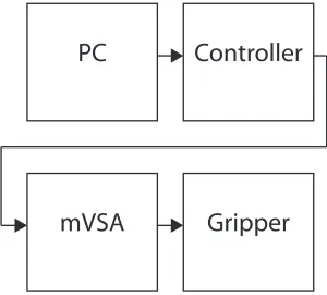
The goal of this project is to integrate the gripper with the mVSA compatible with the robotic manipulator (Figure 3a). The gripper is mechanically redesigned to integrate the variable stiffness mechanism to allow for force tuning on the phalanges. Additionally, modeling, control, and a full construction of the system (Figure 5) is realized.

The report is organized as follows; an overview of the related and previous work is given in section III. Section IV discusses the model and simulations. Section V shows the design of the gripper and supporting components. Section VI describes the methods used. The following section, VII, discusses the results of the experiments. In the last section, conclusion and recommendations are given followed by sug-gested future work. Finally, an appendix is attached including schematics, CAD files and code examples that are not included in the report itself.

(a)Novel gripper design by T.

Bartelds.Source:[4].

(b) Schematic of gripper.

Source:[4].

Fig. 2

(a) Manipulation system by

AQL. Keemink [6] and re-designed by T. Bartelds [4].

Source:[6].

(b) mVSA-UT by E. Barrett

and M. Fumagalli.Source:[5].

Fig. 3

Fig. 4:Gripper and mVSA integration proposal by T. Bartelds. (1) mVSA. (2) Outer output shaft actuating solely a non-compliant position. (3) Compliant output shaft with a controllable stiffness and position. (4) Flexible cable guides carrying the tendons to the end-effector. (5) Pulley to transform forces from the tendons to a torque actuating the finger. (6) The variable compliant tendon. Source:[4].

PC

Controller

mVSA

Gripper

III. PREVIOUS& RELATED WORK

The four-bar linkage gripper design as proposed by T. Bartelds, based on designs discussed in [7] and [8], is the result of a comparison between various under-actuated gripper approaches and has let to the creation of an early proof of concept as shown in Figure 2.

R. Tummers conducted a study, as an extension to [3], in which the aforementioned gripper design has been extended to allow for opening and closing of the fingers using bowden cables [9]. This work adapted the gripper from T. Bartelds to be compatible with the versatile end-effector (Figure 3a).

Since compliant actuation is key to stable and save interac-tion research has led to the development of various compliant actuation systems. Most significant for this project is the work done on the miniature variable stiffness actuator (mVSA) [5] shown in Figure 3b. The mVSA is a miniaturized version of the vsaUT-II [10] [11].

IV. MODEL

(a)Upwards spring (b) Downwards spring

Fig. 6:Studied spring configurations.

To aid in the gripper design and gain insight in its behavior a kinematic and static model has been developed. This is by no means a novel kinematic and static model but an extension on the work by T. Bartelds [4] adapted to design requirements. In this extended model two spring configurations have been studied. The first configuration denotes the upward spring configuration, see Figure 6a. The other configuration considers a downward setup shown in Figure 6b which has already been investigated by T. Bartelds.

The dynamics of the system have not been studied. Ad-ditionally, only a static situation is considered assuming a planar grasp on a cylindrical object. Consequently, results are only valid as long as a full-contact situation (F1, F2 >0) is depicted. The extension also encompasses additional design parameters, most notablys (spring fixture distance) andθof f

which indicates the angle between the pulley mount and the compliant tendon fixture; these parameters allow defining a configuration in which the compliance is DoF invariant. This is further discussed in section IV-E. The resulting gripper schematic is shown in Figure 7.

The design process of the gripper was carried out for the upward spring configuration and as a result most attention is given to this setup. The whole model is shown here, for completeness and understanding, with its additions.

θd θ_p c d a 2 3b 4 3c L₀

L1- L0

L₀ a s robj θ_off 5 6 7 1a 1p b e L2 L1 f

F₁ F2

τa

Fig. 7:Schematic of the gripper model

A. Definitions & assumptions

The definitions and assumptions have not changed with regards to the original model. The range of motion is con-strained:

θd∈[0,0.5π]andθp∈[−

1 4π,

1

4π] (1)

B. Kinematic model

A contact model is considered where the proximal phalanx is always in contact with an object. The two degrees of freedom θp and θd correspond to the opening angle of the

proximal and distal phalanx. A fixed circular object with radius

robj is placed with its center at the symmetry line of the

gripper.

Both the opening angleθp of the proximal phalanx and the

angle of the distal phalanxθdare fixed for a given object size

robj by Eq. (2) and Eq. (3) respectively when a full contact

situation is considered.

θp= 2·arctan _r

obj

L0

−π₂ (2)

θd=π−2·arctan

_r

obj

L1−L0

(3)

6 _{5 = arccos} c

2_+L2 2−e2 2_·c_·L2

!

(4)

6 _{4 =π−}6 _{5 +θd} (5)

d=qL2

1+c2−2·L1·c·cos(6 4) (6)

6 _{2 = arccos} a

2_+b2

−d2 2_·a_·b

!

(7)

6 _{1p= arccos} L

2

1+d2−c2 2·L1·d

!

(8)

6 _{1a= arccos} a

2_+d2_−b2

2_·a_·d

!

6 _{1 =}6 _1a+6 _1p (10)

6 _{3b= arccos} b

2_+d2_−a2

2_·b_·d

!

(11)

6 _{3c= arccos} c

2_+d2_−L2 1 2_·c_·d

!

(12)

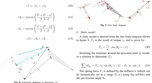
6 _{3 =}6 _3b+6 _3c (13)

c d2 a 2 s θ off 6 1cs b L₁ u v f

Fig. 8:Schematic additions to determine6 _6.

To calculate 6 ₆ two vectors are constructed (see Figure 8, vectors displayed in blue),uandv, from which the following

relationship can be used:

6 _{6 = arccos}

u_·v

ku_{k k}v_k

(14)

For the upward configuration, where the tendon is fixed to a point on the pulley, uandvare given by:

u=

"

(a+f)_·

cos(β1) sin(β1)

−d2·

cos(β2) sin(β2)

# (15) v= " a·

cos(β3) sin(β3)

−d·

cos(β4) sin(β4)

#

(16)

β1=6 1 +θp+θof f

β2=θp+6 1cs

β3=θp+6 1

β4=θp+6 1p

(17)

where:

d2=

q

L2

1+ (c+s)2−2·L1·(c+s)·cos(6 4) (18)

6 _{1cs= arccos} L

2

1+d22−(c+s)2 2·L1·d2

!

(19)

Regarding the downward configuration no specific relation is considered since no design concept has been created to impose constraints, 6 _{6 =−(}6 _{6upward·2)rad}and_{s= 0mm} is used in the simulations.

F1 Fr,y Fr,x L1 L0 a 2 Fb Fa 3b3c

L1- L0

Fs Fb Fr,y Fr,x F2 c s 6 dj pj dj pj

Fig. 9:Free body diagram

C. Static model

A static model is derived from the free body diagram shown in figure 9.Fa is the result of torque τa and is given by:

Fa=

τa

a ·sin θp+6 1

(20)

Summing the moments around the proximal jointpjresults in a relation to determineFb:

X

Mpj =Fa·a·sin θp+6 1−Fb·a·sin6 2 (21)

The spring forceFsis defined by the stiffness k (which can

be dynamically set in a range [0,_∞] using the mVSA) and the pre-tension angle θt:

Fs=k·θt (22)

The moments around distal jointdjare summed to produce a relation forF2:

X

Mdj= Fb·c·sin(6 3)

−Fs·(c+s)·sin (6 3 +6 6) −F2·(L1−L0)

(23)

Force equilibrium for Fr,x andFr,y result in:

Fr,x

Fr,y

+ X

i=b,s,2 Fi·

cos(αi)

sin(αi)

= 0 (24)

Where the angles are defined as:

αb=θp+6 1 +6 2 +π

αs=θp+6 1 +6 2−6 6

α2=θp−θd+

π 2

(25)

Finally F1 can be determined by summing the moments around the proximal jointpj:

X

Mpj= Fr,y·L1·cos(θp) −Fr,x·L1·sin(θp) −F1·L0= 0

F2 F1 F (N ) k(Nmm/rad) τ = 10₀ τ₌ 80 τ = 60 τ = 40 τ = 20

0 5 10 15 20 25

0 0.5 1 1.5 2 2.5 3

Fig. 10:Contact forces for the upward spring configuration for multiple torque values. F2 F1 F (N ) k(Nmm/rad)

τ = 100

τ= 8

0

τ= 6

0

τ= 40

τ=

20

0 5 10 15 20 25

0 0.5 1 1.5 2 2.5 3

Fig. 11:Contact forces for the downward spring configuration for multiple torque values.

D. Simulations

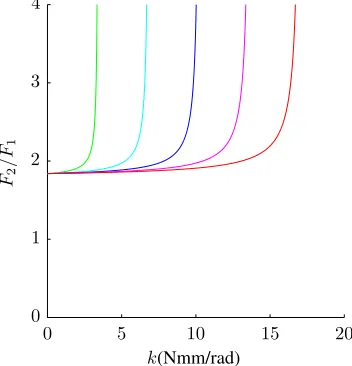
The goal is to allow for force tuning in the phalanges of the gripper. Consequently, simulations are performed using Matlab (v2014a, Mathworks Inc., Natick, USA) to gain insight in the force (ratio) behavior. First the contact forces are calculated and shown in Figure 10 and 11. Subsequently, the force ratio

F2/F1is presented in Figure 12 and 13. Finally, a simulation is carried out to show the behavior of the forces in time when the stiffness is changed; the experiments are conducted using this scenario (see Figure 14 and 15).

The following parameters are used:

a= 10.7mm b= 27.0mm c= 5.0mm e= 24.4mm f = 3.0mm

s= 1.570979mm∨0(upward∨downward configuration)

L0= 15.0mm L1= 30.0mm L2= 20.8mm robj = 20.0mm

θt=1₈π rad

θof f = 0.090403rad

The downward configuration has already been discussed in

a previous project but is added for comparison [4]. Comparing Figure 10 and 11 it is apparent that the spring configuration heavily influences the force behavior. In the upward form changing the stiffness at constant torque decreases both forces while the same action in the downward form cause the proximal phalanx to exert more force while the force on the distal phalanx diminishes. The behavior of the force on the proximal phalanx F2 is identical in both setups while the behavior ofF1is determined by the design. As a consequence the force ratio behavior is different to the same extend as depicted in Figure 12 and 13.

F2

/F

1

k(Nmm/rad)

0 5 10 15 20

0 1 2 3 4

Fig. 12:Contact force ratio in case of the upward spring configuration for multiple torque values.

F2 /F 1 k(Nmm/rad) τ ₌ 100 τ₌ 80 τ = 60 τ ₌ 40 τ₌ 20

0 5 10 15 20

0 0.5 1 1.5 2

Fig. 13:Contact force ratio in case of the downward spring configuration for multiple torque values.

Additionally, Figure 14 and 15 show the behavior in time when the stiffness is changed. This particular situation is recreated in the experiments and used for model validation.

k(Nmm/rad) F2(N)

F1(N)

F o rc e (N ) time(s)

0 1 2 3 0

5 10 15 20 0 1 2 3 4

Fig. 14:Force behavior over time when changing stiffness. Upward spring configuration.τ= 100N mm.

E. Stiffness DoF invariance

In order for the spring force to be invariant of θd and θp

it is required that for any combination of these two degrees of freedom the ratio of the tendon movements snonC

(non-compliant tendon length) and sc (compliant tendon length) is

constant. The ratio between F1 and F2 can be adjusted as long as 6 ₆ is non-zero. If 6 _{6 = 0} the value of _Fb is merely diminished for Fs>0N.

Two design parameters have been chosen for which values can be calculated such that the movement ratio, between the non-compliant and compliant tendon, is constant:sandθof f.

The method is to set up a system of equations for the tendon movements snonC and sc as a function of θp and θd with

adjustable parameters sandθof f:





sc(θp1,θd1) snonC(θp1,θd1)

sc(θp2,θd2) snonC(θp2,θd2)



= "

a+f a a+f

a #

(27)

k(Nmm/rad) F2(N)

F1(N)

F o rc e (N ) time(s)

0 1 2 3 0

5 10 15 20 0 1 2 3 4

Fig. 15:Force behavior over time when changing stiffness. Downward spring configuration.τ= 100N mm.

−20 0 20 40

−30 −20 −10 0 10 20 (a)

−20 0 20 40

−30 −20 −10 0 10 20 (b)

−20 0 20 40

−30 −20 −10 0 10 20 (c)

−20 0 20 40

−30 −20 −10 0 10 20 (d)

−20 0 20 40

−30 −20 −10 0 10 20 (e)

−20 0 20 40

−30 −20 −10 0 10 20 (f)

Fig. 16: Simulated configurations to verify DoF invariance. Dashed red: compliant tendon. Dashed blue: non-compliant tendon.

snonC andsc are defined as:

snonC = ((π−(6 1 +θp))·a)−snonC initial (28)

6 _total=6 _{1 +θp+θof f}

px=cos(6 total)·(a+f)

py =sin(6 total)·(a+f)

phx=d2·cos(θp+6 1cs)

phy =d2·sin(θp+6 1cs)

dt= q

(phx−px)2+ (phy−py)2

sc= ((π−6 total)·(a+f)) +dt−sc initial

(29)

px andpy are the coordinates for the tendon attachment to

the pulley. phx and phy are the coordinates for the tendon

attachment to the distal phalanx. dt is the tendon length

betweenpx,yandphx,y.snonC initialandsc initialare defined

as the tendon lengths atθp = 0.25radandθd= 0rad.

The system from Eq. (27) is numerically solved using

1, θp2 = 0, θd2 = 2. Solutions obtained using the afore-mentioned parameters are s = 1.570979mm and θof f =

0.090403 rad. To verify these values the tendon ratios are computed for most relevant configurations (shown in Figure 16) using the calculated values for s and θof f. The results

(Table I) show an error margin < 1% w.r.t. to the desired fraction a+f

a = 1.280374and thus deemed valid.

TABLE I:Tendon movement ratios for different angles ofθpandθd

for the upward spring configuration. All cases are depicted in Figure 16.

Angle θp= 0.1 θp=−0.1

θd= 0 1.280374 1.280374

θd = 0.25 1.280321 1.280345

θd= 0.5 1.278679 1.279279

V. MECHANICAL DESIGN

All CAD design has been done using SolidWorks (v2014, WolidWorks Corp, Waltham, USA). In this section the (re)design of the mVSA, mVSA housing and gripper is discussed.

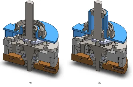
A. mVSA

A minor redesign of the mVSA [5] has been carried out to add a non-compliant (stiff) output aside from the already ex-isting compliant shaft (Figure 17). The stiff output is required to open and close the phalanges.

The mVSA housing is based on original design w.r.t. to tendon fixture by R. Tummers [9]. Additionally, a rotational encoder slot is created to be able to measure the output deflection on the compliant output. The tendons connecting the gripper to the mVSA are routed through bowden cables. The non-compliant and compliant pulleys are designed such that a radii ratio of a+f

a is realized in accordance to the pulley

mechanism in the gripper.

(a)Initial configuration [5]. (b) New configuration with

added non-compliant output.

Fig. 17:mVSA extended non-compliant output, highlighted in blue.

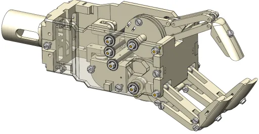
B. Gripper

Using the work carried out by T. Bartelds [4] and R. Tummers [9] as a starting point, a gripper design has been realized (Figure 19) using the parameters calculated in the

(a) (b)

Fig. 18:mVSA motor housing CAD model (a) and combined with mVSA and pulleys (b).

simulations. All iterations in gripper design and mechanical drawings are located in the appendix in Section X-A. All parts except for axes, bearings, nuts, and bolts have been printed in 3D. Nuts and bolts as well as part interlocking proved necessary to make the system strong enough due to the relatively weak nature of the 3D printed material. The tendons are made of Kevlar to prevent elongation and mitigate unwanted compliant behavior.

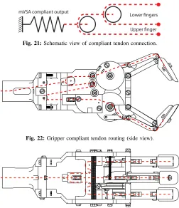
Special attention has been given to the routing of the non-compliant and non-compliant tendons. The non-non-compliant tendon routing is depicted in Figure 20. Due to the asymmetric distribution of the fingers, 1 versus 2, the compliant tendon is connected to all distal phalanges after being routed by a pulley system. This pulley system is schematically depicted in Figure 21. The implementation of this pulley system is shown in Figure 22 and 23 and is a result of careful spacial considerations. Most notably being the length of the entire gripper (from mount to fingers) keeping in mind it is meant to be attached to a UAV off-center (Figure 1). The tendons are attached to the distal phalanges using adjustable nails.

Fig. 19:Gripper CAD model.

Fig. 21:Schematic view of compliant tendon connection.

Fig. 22:Gripper compliant tendon routing (side view).

Fig. 23:Gripper compliant tendon routing (top view).

VI. METHODS

The next section describes the experimental setup, control and calibration, force experiments, and processing of data. First the experimental setup is described followed by the control and calibration. Finally, the experiments and data processing are discussed.

A. Experimental setup

A schematic overview of the experimental setup is shown in Figure 24). Matlab Simulink is installed on a computer and connected via serial to an Arduino Mega 2560 revision 3 (Ar-duino SA) using a newly developed serial connection library. For Simulink, an interface has been created which allows for real-time adjustments of parameters and data acquisition.

The Arduino prototyping board is fitted with a AIRobots interface shield and running a continuous calculation loop at 500Hz. A significant amount of software has been developed for the Arduino board during this project. Where possibly all reusable parts of the software have been re-factored into stand-alone libraries and have been published as open-source on Github. The software is discussed in detail in the appendix.

The mVSA is fitted with two instances of a Pololu 50:1 Mi-cro Metal Gearmotor HP with Extended Motor Shaft (Pololu Corporation, USA) which actually have a transmission ratio of 51.45:1. The motors of the mVSA are connected to the AIRobots interface shield using Pololu High-Power Motor Drivers 18v15. The mVSA is configured with gears resulting in the following transfer function:

φnonC φC =

0.25_·φm0+ 0.375·φC −φnonC−0.706·φm1

(30)

The upper phalanges are fitted with FSR-400 (Interlink Electronics, Canada) force sensitive resistors. These force sensors are connected by a voltage divider to the Arduino (schema available in Section X-D). The measuring resistorRm

on the voltage divider is chosen to maximize the desired force sensitivity range and to limit current.

The tendons fitted on the gripper are connected to the mVSA using bowden cables which also allow for proper tensioning.

A hardware interface board has been created to allow for easy manual control of the system (see Section X-C).

B. Control and calibration

For the mVSA setpoints are generated using a trapezoidal motion profile (discussed in X-G). From these angular set-points the motor steps are calculated from the mVSA transfer function and controlled using a manually tuned PID controller. A state manager is used to control switching between startup, calibration, manual control, and Simulink interface states.

Calibration of the open and closed position of the gripper is performed by slowly opening and closing until the endpoints are detected using software methods.

C. Force measurement experiments

During the force experiments a ping-pong ball wound in isolation tape (Figure 28), to provide a more stable contact between the force sensors and the ball, is placed between the fingers. Force is applied by the mVSA to ensure a full-contact situation. Finally, the compliant output stiffness is changed to mimic the simulated cases for comparison and validation.

The measurements (notably the output voltage Vout) were

captured in Matlab and processed to calculate the actual forces exerted on the sensors. The variable resistance of the FSR is related to the measured input voltage by:

Vout=

Vcc·Rm

Rm+Rf s

(31)

WhereRm= 30kΩandVcc= 5V. The FSR resistance in

terms of these parameters is:

Rf s=

(Vcc−Vout)·Rm

Vout

(32)

From the calibration data provided by the manufacturer a very close approximation has been calculated using Microsoft Excel invoking a power fit resulting in the following relation-ship:

F = 296852_·R

−0.825

f s

Fig. 25:Experimental setup overview.

Fig. 26:mVSA + housing.

Fig. 27:Gripper.

Fig. 28:Gripper showing FSR attachment.

1

2

3

5

4

6

11

15

16

14

17

12

13

9

₁₀

8

7

VII. DISCUSSION

In this section the results from the experiments are reviewed. At first, encountered difficulties and errors are considered. Secondly and finally, the measurements are presented and discussed.

A. Difficulties and common errors

Friction is a significant factor in the system. This can be attributed to the non-compliant tendon thickness and stiff-ness, usage of bowden cables for both the non-compliant and compliant tendons. While friction in bowden cables is usually minor, it does have influence on forces on this scale. Additionally, the 3D printed material has a relatively high coefficient of friction. This has been minimized as much as possible by the usage of bearings, nylon spacers and specific tolerances to reduce self-contact.

Matlab Simulink proved to be fairly unstable in 64-bit mode on Microsoft Windows. The system crashed on seemingly random moments. Many times the experiments had to be rerun due to crashes. Issues were reported on-line with this type of setup using the 64-bit version of Matlab in combination with the Real-time target features and is reportedly subject to investigation likely to be fixed and/or mitigated in subsequent releases of Matlab.

The effects of symmetrical or asymmetrical amount of fingers configuration has not been investigated. The compliant tendon pulley system is designed to make it invariant of the amount of fingers but this has not been experimentally verified. Every time the experiment was conducted there were minor differences in the initial compliant offset. This was because the rotational sensor to measure the compliant output deflection was not used due to technical difficulties and time constraints. The offset was manually applied and although closely approx-imated not guaranteed to be the same every time.

Force sensitive resistors (FSR) are known to be inaccurate w.r.t. repeatability, temperature influences, and inhomogeneous loading issues. It is a cheap method of force sensing but careful calibration is required to get somewhat accurate results. In these experiments the calibration values from the manufacturer is used, which are only a rough approximation.

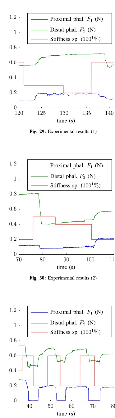
B. Force behavior

Experimental results are shown in Figure 29, 30 and 31. Most importantly the behavior seen in the simulations re-garding the effect of increasing stiffness causing a decrease in forces is equally apparent in the experiments as well. The repeatability within a single experiment is apparent from Figure 31.

A consistent lag can be observed in all experiments. The lag is mainly attributed to the use of a motion profile generator (which limits the acceleration and speed) and significant friction in the system.

The force ratio, as simulated, expects a larger range of the

F2values compared toF1. The experiments revealed identical behavior in the first two shown cases. The third case seems to indicate a relatively equal range of both forces. This may be caused by inaccurate pretensioning of the compliant output.

Stiffness sp. (1001_%)

Distal phal.F2(N)

Proximal phal.F1(N)

time (s)

120 125 130 135 140

0 0.2 0.4 0.6 0.8 1 1.2

Fig. 29:Experimental results (1)

Stiffness sp. (1001_%)

Distal phal.F2(N)

Proximal phal.F1(N)

time (s)

70 80 90 100 110

0 0.2 0.4 0.6 0.8 1 1.2

Fig. 30:Experimental results (2)

Stiffness sp. (1001_%)

Distal phal.F2(N)

Proximal phal.F1(N)

time (s)

40 50 60 70 80

0 0.2 0.4 0.6 0.8 1 1.2

VIII. CONCLUSIONS& RECOMMENDATIONS

A. Conclusions

A mechanical redesign of the gripper with the addition of a variable spring has been realized. Additionally, an existing kinematic and static model have been extended and verified based on the new design. The mVSA has been redesigned adding a stiff output besides the already existing compliant output. Result is a complete integration between the gripper and mVSA, and control and construction of the whole system. The model, which behavior is verified by experiments, shows that it is possible to tune both the forces and force ratio exerted by the phalanges of an under-actuated gripper.

B. Recommendations

The current force sensing setup using a ball gives too many problems in the sense that it is hard to ensure a homogeneous force distribution on the sensor surfaces. Other problems were compliance, friction, and slip on the ball. The FSR (force sensitive resistor), while cheap and easy to use, requires careful placement. An improved setup is depicted in Figure 32.

(a)Current measurement setup

using a ping-pong ball (b)setup. Dashes indicate the sym-Suggested measurement metry line.

Fig. 32:Force sensing recommendation

Additionally, it may be worth looking into alternative force sensing techniques which may involve more sophisticated sensors.

The current pulley system, especially for the compliant tendon, needs a lot of space. A setup which uses tendons/cable guides instead of the current pulley system may be a more stable solution and will probably make the gripper smaller and more reliable. Figure 33 shows a concept.

Pulley system

Fig. 33:Gripper compliant tendon routing proposal.

The 3D printed material has noticeable limits on strength, weight, and tolerances which will make further miniaturization

hard to carry out. Other materials may be required and can be investigated.

IX. FUTURE WORK

A different force control method is required in order to set a desired force (ratio) on the phalanges. The series elastic actuator approach may aid in developing alternative control methods [13].

Currently, only a symmetric non-compliant shape has been investigated. Other shapes and control methods are required to allow for adaptive gripping on uneven, rugged, compliant and undulating surfaces typically found in the natural world. Addi-tionally, different grasping techniques (for example pinching) can be researched by extending the current setup.

Implications of the geometric choices (e.g. the upward and downward spring configurations) should be more carefully examined. It may be interesting to find out which configuration is favorable over another considering different scenarios.

The development of a 20-sim model to study dynamics can be investigated and may provide more insight. There is already a 20-sim model available for the mVSA and for the gripper created by R.Tummers. These can be integrated which may be relatively easy since the current gripper 20-sim model contains a static spring which can be changed to a variable version. The model is currently setup for a spring configuration in which it is attached to two joints in a downward configuration.

REFERENCES

[1] EC, “Airobots,” 2013, innovative aerial service robots for remote inspections by contact. [Online]. Available: http://airobots.ing.unibo.it/ Home.php

[2] ——, “Sherpa project,” 2014, innovative aerial service robots for remote inspections by contact. [Online]. Available: http://www.sherpa-project. eu/

[3] M. Fumagalli, “Quadrotor interacting with a remote environment: Con-trol of a flying hand”.”

[4] J. Bartelds, “Design and control of a modular end-effector for uavs in interaction with a remote environment,” 2012.

[5] M. Fumagalli, E. Barrett, S. Stramigioli, and R. Carloni, “The mvsa-ut: A miniaturized differential mechanism for a continuous rotational variable stiffness actuator,” inBiomedical Robotics and Biomechatronics (BioRob), 2012 4th IEEE RAS & EMBS International Conference on. IEEE, 2012, pp. 1943–1948.

[6] A. Keemink, M. Fumagalli, S. Stramigioli, and R. Carloni, “Mechanical design of a manipulation system for unmanned aerial vehicles,” in Robotics and Automation (ICRA), 2012 IEEE International Conference on. IEEE, 2012, pp. 3147–3152.

[7] T. Lalibert´e, L. Birglen, and C. Gosselin, “Underactuation in robotic grasping hands,”Machine Intelligence & Robotic Control, vol. 4, no. 3, pp. 1–11, 2002.

[8] S. Krut, “A force-isotropic underactuated finger,” inRobotics and Au-tomation, 2005. ICRA 2005. Proceedings of the 2005 IEEE International Conference on. IEEE, 2005, pp. 2314–2319.

[9] R. Tummers, “Design of control strategies for uavs physically interacting with each other and the environment,” 2012.

[10] S. S. Groothuis, G. Rusticelli, A. Zucchelli, S. Stramigioli, and R. Car-loni, “The vsaut-ii: A novel rotational variable stiffness actuator,” in Robotics and Automation (ICRA), 2012 IEEE International Conference on. IEEE, 2012, pp. 3355–3360.

[11] ——, “The variable stiffness actuator vsaut-ii: Mechanical design, modeling, and identification,”Mechatronics, IEEE/ASME Transactions on, vol. 19, no. 2, pp. 589–597, 2014.

[12] Pololu, “50:1 micro metal gearmotor hp with extended motor shaft,” jun 2014. [Online]. Available: https://www.pololu.com/product/2213/specs [13] H. Vallery, R. Ekkelenkamp, H. Van Der Kooij, and M. Buss, “Passive

X. APPENDIX

A. Technical drawings: Gripper

This section contains an iteration overview and relevant technical drawings for the gripper. The final CAD model is shown in Figure 34. All design iterations leading up to the final model are shown in section X-A1 accompanied by the most important mechanical drawings of the final design.

All CAD files are available at the Robotics and Mechatronics group at the University of Twente.

1) Design iterations:

(1)Original design by Teun Bartelds [4]. (2)Improved design by Ramon Tummers [9].

(3)Iteration #1 (4)Iteration #2

(5)Iteration #3 (6)Iteration #4

(7)Iteration #5 (8)Iteration #6

36

2

2,50

Back

Isometric

42,68

Top

2

2

19,80

Right

FACULTY OF ENGINEERING PROJECTION

METHOD DATE

MATERIAL TITLE

SURFACE FINISH

DRAWING NO.

REV.

DIMENSIONS IN MILLIMETERS SHEET 1 OF 1

A4

SCALE CHECKED

--28-1-2015 1:1

01

--Wrist

Wrist_v2

FILE / PART NAME

--Isometric

26

9

3 6

2

7

15

10

8,50

6,50

25,20

36,50

13

5

4

11,50

7,50

10,31

8

92,01

4

8

1,20

4,50

Back

Right

Top

FACULTY OF ENGINEERING

PROJECTION

METHOD DATE

MATERIAL TITLE

SURFACE FINISH

DRAWING NO.

REV.

DIMENSIONS IN MILLIMETERS SHEET 1 OF 1

A4

DRAWN

SCALE CHECKED

--28-1-2015 1:1

01

--Left side

BaseSideLeft

FILE / PART NAME

--Isometric

41,80

6,54

4

4

3

₆

9

1

3

35,80

5

23,80

7,83

4

0,50

2,30

1,20

3,90

18

26

4

5

1

2

2

Top

Right

FACULTY OF ENGINEERING PROJECTION

METHOD DATE

MATERIAL TITLE

SURFACE FINISH

DRAWING NO.

REV.

DIMENSIONS IN MILLIMETERS SHEET 1 OF 1

A4

DRAWN

SCALE CHECKED

--28-1-2015 1:1

01

--Tendon pulley block

SidePulleys_Full FILE / PART NAME

14,60

10,60

7,50

7,50

_8,50

11,50

4

10,60

21,20

29,71

23,71

1,20

3,90

36

2

49,80

5

4

2

Right

Top

Isometric

FACULTY OF ENGINEERING

PROJECTION

METHOD DATE

MATERIAL TITLE

SURFACE FINISH

DRAWING NO.

REV.

DIMENSIONS IN MILLIMETERS SHEET 1 OF 1

A4

DRAWN

SCALE CHECKED

--28-1-2015 1:1

01

--Base

Base

FILE / PART NAME

--B. Technical drawings: mVSA

The original mVSA design has been adapted to support a non-compliant output shaft. Differences are shown in Figure 36. The mechanical drawing for the updated frame is added at the end of this section.

(a) (b)

.

2,42

1,50

_2,30

10

11,90

1

4,30

13,58

0,20

R14

7

10

12

2,20

1

Top

Back

Top

FACULTY OF ENGINEERING

PROJECTION

METHOD DATE

MATERIAL TITLE

SURFACE FINISH

DRAWING NO.

REV.

DIMENSIONS IN MILLIMETERS SHEET 1 OF 1

A4

DRAWN

SCALE CHECKED

--28-1-2015 2:1

01

--Frame

frame-a

FILE / PART NAME

--C. Electronics: Interface board

A simple interface has been designed which has the ability to indicate the current active state using LED’s, discrete input using two buttons and analogue input using two potentiometers.

Fig. 37:Realization of the interface board.

D. Electronics: Force sensor interface

A simple interface, shown in Figure 39, between the Arduino board and force sensors.

E. Software: Overview

A significant amount of software has been developed for this project to run on the Arduino Mega 2560 board. Worth noting is the usage of the AVR-STL1 _{library on the Arduino board allowing for easier memory management and data handling.}

Where possible, the software was re-factored into standalone libraries and published as open-source on Github if they were considered useful to others. In the following sections it will be explicitly noted if the source code is publicly available.

F. Software: Simulink interface

A dedicated Matlab Simulink interface has been created to allow for easy parameter adjustments, logging, control and data acquisition. It is connected to the Arduino board using the Matlab real-time target functionality. Serial communication on the Arduino is handled by a newly created library discussed in Section X-I.

G. Software: Motion profile generation

Source code and documentation is available on Github.2

A motion-profile generator has been designed to calculate the position setpoints for the mVSA motors in a predictable less-jerky manner. This method creates a trapezoidal motion profile to reach a given setpoint while adhering to a given maximum velocity and acceleration. The generator is able to both calculate a complete path beforehand and generating it on the fly based on the current position and velocity.

The trapezoidal method has first been developed in Matlab (see Figure 41) and once it worked, implemented and experimentally verified on the system (mVSA) in C++ (see Figure 43-46). Additionally, aconstant velocityprofile method has

been created and implemented as well (see Figure 42). The actual velocity measured in the experiments has been smoothed using a Gaussian kernel for easier comparison with the simulated velocity.

Fig. 41:Simulation of trapezoidal motion for given setpoints. Maximum velocity is set at 0.15m/sand the maximum acceleration is set at 0.1m/s2_.

Jerk

(s)

(

m

/s

3)

Acceleration

(s)

(

m

/s

2)

Velocity

(s)

(

m

/s

)

Position Setpoint

(s)

(

m

)

0 1 2 3 4 5 6

0 1 2 3 4 5 6

0 1 2 3 4 5 6

0 1 2 3 4 5 6

×105

−1

0 1

−100

0 100

−0.2

0 0.2 0 0.5 1

Actual velocity - GK / RBF smooth Simulated velocity

Simulated position

(s)

(d

eg

re

es

)

Actual velocity - GK / RBF smooth Actual velocity

Actual position Setpoint

Generated position

(s)

(d

eg

re

es

)

0 1 2 3 4 5 6

0 1 2 3 4 5 6

0 200 400 600 800 0 200 400 600 800

Fig. 43:Experiment and model verification using a constant setpoint.

Actual velocity - GK / RBF smooth Simulated velocity

Simulated position

(s)

(d

eg

re

es

)

Actual velocity - GK / RBF smooth Actual velocity

Actual position Setpoint

Generated position

(s)

(d

eg

re

es

)

0 1 2 3 4 5 6 7 8 9 10 11

0 2 4 6 8 10

−200 0 200 400 600 800

−200 0 200 400 600 800

Actual velocity - GK / RBF smooth Simulated velocity

Simulated position

(s)

(d

eg

re

es

)

Actual velocity - GK / RBF smooth Actual velocity

Actual position Setpoint

Generated position

(s)

(d

eg

re

es

)

0 2 4 6 8 10 12 14 16 18

0 5 10 15

−200 0 200 400 600 800

−200 0 200 400 600 800

Fig. 45:Experiment and model verification using a variable setpoint.

Listing 1:MotionProfile usage example

1 #include "MotionProfile.h" 2

3 /**

4 * Initialization

5 *

6 * @param int aVelocityMax maximum velocity (units/s)

7 * @param int aAccelerationMax maximum acceleration (units/sˆ2)

8 * @param short aMethod method of profile generation (1 = trapezoidal)

9 * @param int aSampleTime sample time (ms)

10 */

11 MotionProfile trapezoidalProfile = new MotionProfile(200, 100, 1, 10);

12

13 /**

14 * Usage

15 */

16 // Update setpoint for profile calculation and retrieve calculated setpoint

17 float finalSetpoint = 1000;

18 float setpoint = trapezoidalProfile->update(finalSetpoint)

19

20 // Check if profile is finished

21 if (trapezoidalProfile->getFinished()) {};

22

23 // Reset internal state

H. Software: Magnetic switch center determination

Magnetic switches are used to calibrate the mVSA frame and pivot position. These switches exhibited two types of behavior: single and double dip. A method was created which recognizes and determines the center point in both cases. The method was first developed and tested in Matlab and once verified implemented in C++ for usage on the Arduino micro-controller.

In the matlab code, first the transition points are detected using getTransitionPoints and this is used as input for the findCenter function which determines the actual center. In the

C++ code a single function handles all calculations.

Angle (θ) case 3 Angle (θ)

case 2 Angle (θ)

case 1

0 100 200 300

0 100 200 300

0 100 200 300

−1

0 1 2

−1

0 1 2

−1

0 1 2

Fig. 47:Single dip simulation for the three possible cases. Green dots denote the transition points. Red dots denote the determined center.

Angle (θ) case 5 Angle (θ)

case 4 Angle (θ)

case 3 Angle (θ)

case 2 Angle (θ)

case 1

0 100 200 300

0 100 200 300

0 100 200 300

0 100 200 300

0 100 200 300

−10

1 2

−10

12

−10

12

−10

1 2

−01

12

Listing 2:getTransitionPoints.m

1 % Transition point function

2 function R = getTransitionPoints(A, default)

3 previous = default;

4 R = [];

5

6 % Loop values to find transition points

7 for i = 1:size(A,1)

8 if A(i, 2) ˜= previous

9 % Check if this is the first entry, if so, it's not a change

10 if i == 1

11 previous = A(1,2);

12 else

13 R(end + 1) = A(i,1);

14 previous = A(i,2);

15 end

16 end

17 end

18 end

Listing 3:findCenter.m

1 % Center function

2 function center = findCenter(A, length)

3 count = size(A,2)

4 dist = zeros(1, count)

5

6 % Calculate all distances

7 for i = 1:count

8 if i < count

9 dist(1, i) = abs(A(i) - A(i + 1));

10 else

11 % Last value, wrap around

12 dist(1, i) = abs(A(i) - length - A(1));

13 end

14 end

15

16 % Get smallest distance

17 [val, locn] = min(dist)

18

19 % Calculate center

20 center = mod(A(locn) + round(val / 2), length);

21 end

Listing 4:findCenter.cpp

1 /*

2 * FUNCTION: findCenter

3 * Determines the amount of free ram available

4 * @param v vector containing the transition points.

5 * @param length total amount of points (e.g. 360 if using degrees)

6 * E.g. [10, 20, 50, 100], 120 will return 15

7 * @return center point

8 */

9 int findCenter (std::vector<int>& b, int length, bool modulus = true) {

10 std::vector<int> distancePoints;

11

12 // Calculate all distances

13 for(std::vector<int>::size_type i = 0; i != b.size(); i++) {

14 if (i < b.size() - 1) {

15 distancePoints.push_back(abs(b[i] - b[i + 1]));

16 }

17 else {

18 // Last value, wrap around

19 distancePoints.push_back(abs(b[i] - length - b[0]));

20 }

21 }

22

23 // Get the smallest distance

24 int smallestIndex = 0;

25 int smallestValue = INT_MAX;

26 for(std::vector<int>::size_type j = 0; j != distancePoints.size(); j++) {

28 smallestValue = distancePoints[j];

29 smallestIndex = j;

30 }

31 }

32

33 // Calculate the center

34 // If the modulus produces wrong/weird results, see: ...

https://stackoverflow.com/questions/2581594/how-do-i-do-modulus-in-c

35 int returnValue = (b[smallestIndex] + round(smallestValue / 2));

36

37 if (modulus) {

38 returnValue %= length;

39 }

40 return returnValue;

I. Software: Simulink serial connector

Source code and documentation is available on Github.3

The simulink serial connection library has been created due to both the lack of a standard approach and as a training exercise to learn about serial communication protocols.

Listing 5:SimulinkConnector usage example

1 #include "SimulinkConnector.h" 2

3 /**

4 * Initialization

5 *

6 * The output format accepts the following types:

7 * l = long

8 * ul = unsigned long

9 * u = unsigned int

10 * i or d = int

11 * Multiple datatypes can be used at once, however,

12 * the sendPacket() function only accepts long types.

13 * You can use casting to transmit the other datatypes.

14 *

15 * @param aOutputFormat char string containing the output format; e.g. "S %d %l %ul E".

16 * @param aInputPacketVector vector to which serial input will be written

17 * @param aOutputPacketVector vector from which output serial is composed

18 * @param aOutputInterval sample time of serial output in milliseconds

19 */

20 std::vector<long> outputPacketVector(5,0);

21 // Configured an output of 5 long values from Matlab Simulink

22 std::vector<long> receivedPacketVector(5,0);

23 SimulinkConnector simulinkConnection("S %l %l %l %l %l E", receivedPacketVector, ...

outputPacketVector, 20);

24

25 /**

26 * Usage

27 */

28 // Arduino loop

29 simulinkConnection.update();

30

31 // Set output variables (at any point in the loop or supporting function):

32 outputPacketVector[0] = 99;

33

34 // Read input variables (this is always accessible after initialization):

35 int incomingValue = receivedPacketVector[2] // Read third value of incoming data vector

J. Software: Memory efficient logger

Source code and documentation is available on Github.4

This library is a fork from the Arduino logging library.5_{Support has been added for theFlashStringHelperdata type which} enables the logging of strings (which can take up considerable space, especially when adding a lot of log statements) saved to the flash program space memory (PROGMEM) instead of the scarce SRAM. This enables us to add a significant amount of log statements while almost no scarce SRAM is needed.

Listing 6:Logging usage example

1 #include <Logging.h>

2

3 /**

4 * Initialization

5 *

6 * Setup logging, available is:

7 * 0 LOG_LEVEL_NOOUTPUT no output

8 * 1 LOG_LEVEL_ERRORS only errors

9 * 2 LOG_LEVEL_INFOS errors and info

10 * 3 LOG_LEVEL_DEBUG errors, info and debug

11 * 4 LOG_LEVEL_VERBOSE all

12 *

13 */

14 const int LOG_LEVEL = LOG_LEVEL_INFOS;

15 const long BAUD_RATE = 115200; // Serial transmission rate in bits per second;

16 Log.Init(LOG_LEVEL, BAUD_RATE);

17

18 /**

19 * Usage

20 */

21 // Debug logging, not shown since current log level is LOG_LEVEL_INFOS

22 Log.Debug(F("Pin %d selected as debug output pin\n"), 1);

23

24 // Log info, is shown since log level is LOG_LEVEL_INFOS

25 Log.Info(F("******************************************\n"));

26 Log.Info(F("Setup arduino complete\n"));

27 Log.Info(F("Initiating first stage...\n"));

28 Log.Info(F("******************************************\n"));

K. Software: State manager

Source code and documentation is available on Github.6

Manager library for an existing state library.7 _{Enables easy usage with Arduino.}

Listing 7:Statemanager usage example

1 #include "Statemanager.h" 2

3 /**

4 * Initialization

5 *

6 * @param byte [buttonStateSwitchPin] pin number of button that switches the states.

7 * @param byte stateVector Vector containing all initial states.

8 */

9 // Create vector with states

10 const State stateArr[] = {

11 State(STATE_IDLE_ENTER, STATE_IDLE_UPDATE, STATE_IDLE_EXIT),

12 State(STATE_MVSACALIBRATION_UPDATE),

13 State(STATE_GRIPPERCALIBRATION_ENTER, STATE_GRIPPERCALIBRATION_UPDATE, ...

STATE_GRIPPERCALIBRATION_EXIT),

14 State(STATE_GRIPPERSIMULINK_MODE1_ENTER, STATE_GRIPPERSIMULINK_MODE1_UPDATE, ...

STATE_GRIPPERSIMULINK_MODE1_EXIT)

15 };

16

17 // Initialize the stateManager with the states

18 std::vector<State> statesVector (stateArr, stateArr + sizeof(stateArr) / sizeof(stateArr[0]) );

19 StateManager stateMngr = StateManager(BUTTON_STATESWITCH_PIN, statesVector);

20

21 /**

22 * Usage

23 */

24 // In the Arduino loop

25 void loop()

26 {

27 // Check states (check which one is active and run the update function)

28 stateMngr.checkStates();

29 }

30

31 // Transition to next state

32 stateMngr.transitionToNextState();

6_{https://github.com/WRidder/Arduino-StateManager}

L. Software: PID Controller

Source code and documentation is available on Github.8

This PID library only supports the long data-type, preventing floating point operations, in order to speed up setpoint

calculations. This is a fork from the original Arduino PID library. Additionally, some small features like error margins and obstruction detection have been added.

Listing 8:PID usage example

1 #include "PID_Extended_Controller.h" 2

3 /**

4 * Initialization

5 *

6 * @param long P proportional gain

7 * @param long I proportional gain

8 * @param long D proportional gain

9 * @param int Dir direction

10 */

11 PIDController pid = PIDController(1, 0.1, 0.02, 0);

12

13 /**

14 * Usage

15 */

16 // Set control variables

17 long* InputAngle;

18 long_{* Output;} 19 long* Setpoint;

20 InputAngle = new long(0.0);

21 Output = new long(0.0);

22 Setpoint = new long(0.0);

23 pid.SetControlVariables(long* InputAngle, long* Output, long* Setpoint)

24

25 // Update input variables

26 InputAngle = sensorReading();

27

28 // Compute PID output

29 pid.Compute();

30

31 // Use output

32 setMotorDutyCycle(*Output);

M. mVSA calibration

The mVSA is calibrated in two steps. First the frame position is determined by slowly opening and closing the fingers and using software methods for end-point detection. Secondly, the compliant output is calibrated using magnetic switches in the housing of the mVSA.

The full calibration routine is depicted in Figure 49.

Measured M1 Setpoint M1 Measured M0 Setpoint M0 (s) (s te p s)

Motor setpoints and measurements

Switch Pivot MP Setpoint Pivot Setpoint Pivot Pivot calibration (s) (d eg re es ) Switch Frame MP Setpoint Frame Setpoint Frame Frame calibration (s) (d eg re es ) (d ig it al h i/ lo ) (d ig it al h i/ lo )

0 5 10 15 20 25 30

0 5 10 15 20 25 30

0 5 10 15 20 25 30

0 5 10 15 20 25 30

0 5 10 15 20 25 30

×104

−1

−0.5 0 0.5 1 0 200 400 600 800 1000 0 200 400 600 800 1000 0 1 0 1