Michigan Technological University Michigan Technological University
Digital Commons @ Michigan Tech
Digital Commons @ Michigan Tech
Dissertations, Master's Theses and Master's Reports
2018
System Architecture Optimization Using Hidden Genes Genetic
System Architecture Optimization Using Hidden Genes Genetic
Algorithms with Applications in Space Trajectory Optimization
Algorithms with Applications in Space Trajectory Optimization
Shadi Ahmadi DaraniMichigan Technological University, [email protected]
Copyright 2018 Shadi Ahmadi Darani
Recommended Citation Recommended Citation
Ahmadi Darani, Shadi, "System Architecture Optimization Using Hidden Genes Genetic Algorithms with Applications in Space Trajectory Optimization", Open Access Dissertation, Michigan Technological University, 2018.
SYSTEM ARCHITECTURE OPTIMIZATION USING HIDDEN GENES GENETIC ALGORITHMS WITH APPLICATIONS IN SPACE TRAJECTORY
OPTIMIZATION
By
Shadi A. Darani
A DISSERTATION
Submitted in partial fulfillment of the requirements for the degree of DOCTOR OF PHILOSOPHY
In Mechanical Engineering-Engineering Mechanics
MICHIGAN TECHNOLOGICAL UNIVERSITY 2018
This dissertation has been approved in partial fulfillment of the requirements for the Degree of DOCTOR OF PHILOSOPHY in Mechanical Engineering-Engineering Mechanics.
Department of Mechanical Engineering-Engineering Mechanics
Dissertation Advisor: Dr. Ossama Abdelkhalik
Committee Member: Dr. Nilufer Onder
Committee Member: Dr. Nina Mahmoudian
Committee Member: Dr. Mo Rastgaar
Dedication
Contents
List of Figures xi
List of Tables xv
Preface xvii
Acknowledgments xix
List of Abbreviations xxi
Abstract xxiii
1.1 Overview . . . 1
1.2 Genetic Algorithms . . . 4
1.3 Space Trajectory Optimization . . . 8
1.4 Motivations and Objectives . . . 12
1.5 Organization of the Dissertation . . . 14
2 Hidden Genes Genetic Algorithms 15 2.1 Introduction . . . 15
2.2 Modeling Genes and Chromosomes . . . 16
2.3 Hidden Genes in Biology . . . 17
2.4 Concept of HGGAs in Optimization . . . 19
2.5 Conclusion . . . 21
3.2 HGGAs Mechanisms . . . 24
3.3 Conclusion . . . 31
4 Test Cases 33 4.1 Introduction . . . 33
4.2 VSDS Mathematical Functions . . . 34
4.3 Space Trajectory Optimization . . . 41
4.3.1 Earth to Mars Mission Trajectory Optimization . . . 52
4.3.2 Earth to Jupiter Mission Trajectory Optimization . . . 59
4.3.3 Earth to Saturn (Cassini 2) Mission Trajectory Optimization . 65 4.4 Discussion . . . 68
4.5 Conclusion . . . 78
5 Convergence Analysis 81 5.1 Introduction . . . 81
5.2 Markov Chain Model of Genetic Algorithms . . . 83
5.3 Markov Chain Model of Hidden Genes Genetic Algorithm . . . 90
5.3.1 Selection Matrix S . . . 91
5.3.2 MutationM and Crossover C Matrices . . . 93
5.4 Numerical Analysis . . . 104
6 Conclusion 107 6.1 Dissertation Summary and Conclusion . . . 107
References 111
List of Figures
1.1 Interplanetary Trajectory Optimization Problem Topology . . . 2
2.1 In standard GA, a chromosome (code) is a string of genes that represent a solution . . . 16
2.2 Chemical tags (purple diamonds) and the ”tails” of histone proteins (purple triangles) mark DNA to determine which genes will be tran-scribed. (picture is modified from [1]) . . . 18
2.3 Hidden genes and effective genes in two different chromosomes [2] . . 19
2.4 Crossover operation in HGGA [2] . . . 21
3.2 Schematic of Mechanism A . . . 25
3.3 Representation of arithmetic crossover in IR3. . . 26
3.4 Schematic of Mechanism B. . . 27
3.5 Schematic of Alleles Mechanism. . . 29
3.6 Schematic of Logic A. . . 30
3.7 Schematic of Logic B. . . 30
3.8 Schematic of Logic C. . . 31
4.1 Success rate of some mechanisms in Egg Holder function. . . 38
4.2 Box diagram of all the mechanisms in Egg Holder function. . . 39
4.3 Geometry of a non-powered flyby. . . 44
4.4 The local and inertial frames [3]. . . 47
4.5 An example of two different solutions for an interplanetary trajectory problem in HGGA (Earth to Jupiter), and the equivalent chromosomes
4.6 Zero-DSM and MGADSM trajectories for Earth to Mars mission using mechanism H. . . 56
4.7 Zero-DSM and MGADSM trajectories for Earth to Mars mission using alleles concept. . . 57
4.8 Box diagram of all the mechanisms in Earth to Mars problem (MGADSM phase). . . 58
4.9 Zero-DSM and MGADSM trajectories for Earth to Jupiter mission using mechanism E. . . 61
4.10 Zero-DSM and MGADSM trajectories for Earth to Jupiter mission using mechanism H. . . 62
4.11 Evolution of tags using Logic C in the Earth to Jupiter problem . . . 63
4.12 Box diagram of all the mechanisms in Earth to Jupiter problem (MGADSM phase). . . 64
4.13 MGADSM trajectory for Earth to Saturn mission using mechanism H. 68
4.14 Success rate of the proposed mechanisms in the Earth to Mars problem (MGADSM model). . . 71
4.15 Success rate of the proposed mechanisms in the Earth to Jupiter prob-lem (MGADSM model). . . 73
4.16 Cost value vs. pericenter altitude of first flyby for Cassini 2 mission . 75
5.1 Numerical Convergence of 5 simulations in Earth to Mars problem (zero-DSM model) using logic A. . . 105
5.2 Numerical Convergence of 5 simulations in Earth to Jupiter problem (MGADSM model) using mechanism D. . . 105
List of Tables
1.1 Design variables in an interplanetary trajectory optimization problem 9
4.1 Genetic Algorithm Options . . . 36
4.2 Egg Holder function results . . . 40
4.3 Schwefel 2.26 function results . . . 40
4.4 Styblinski-Tang function results . . . 41
4.5 Design variables in an interplanetary trajectory optimization problem 42 4.6 Lower and upper bounds of Earth-Mars problem . . . 54
4.7 Results of Earth-Mars problem in zero-DSM phase. . . 55
4.9 Solution of Earth to Mars mission (EVM) using mechanism H . . . . 57
4.10 Solution of Earth to Mars mission (EVM) using alleles concept . . . . 58
4.11 Lower and upper bounds of Earth-Jupiter problem . . . 59
4.12 Results of Earth-Jupiter problem in zero-DSM model . . . 60
4.13 Results of Earth-Jupiter problem in MGADSM model . . . 61
4.14 Solution of Earth to Jupiter (EVEJ) mission using mechanism E . . . 62
4.15 Solution of Earth to Jupiter (EVEJ) mission using mechanism H . . . 63
4.16 Lower and upper bounds of Earth-Saturn problem . . . 66
4.17 Success rates of Earth-Saturn problem in zero-DSM model . . . 67
4.18 Results of Earth-Saturn problem in MGADSM model . . . 68
4.19 Solution of Earth to Saturn (EVVEJS) mission using mechanism H . 69
Preface
The publications in this dissertation are part of the research carried out during my PhD studies at Michigan Technological University during 2015-2018. The optimiza-tion algorithms developed in this dissertaoptimiza-tion can be used in various problems in robotics, aerospace, electrical, etc. fields. Some examples of these applications are provided in Section 1.1 and some mathematical and space trajectory optimization problems are investigated in details in Chapter 4.
Chapter 1 presents the overview of the dissertation, motivations and objective of the work, and the organization of this thesis. The content of this chapter has been published in References [4, 5]. Chapter2 presents the concept of hidden Genes Ge-netic Algorithm in biology and optimization. The content of this chapter has been published in References [4, 6, 7]. Chapter 3 presents the proposed mechanisms for selecting the hidden genes. The content of this chapter has been published in Refer-ences [6, 8]. Chapter 4 presents mathematical test cases and three space trajectory optimization problems. The mechanisms proposed in chapter 3 are tested on these problems and the results are compared to the literature. The content of this chapter has been published in References [4, 5, 6, 7]. Chapter 5 presents the Markov Chain convergence analysis of the proposed mechanisms and it is proven that the proposed mechanisms satisfy minimum conditions for convergence. The content of this chapter
Acknowledgments
I would like express my sincere gratitude to Dr. Ossama Abdelkhalik for his contin-uous support, advice, and encouragement.
I with to thank the members of my dissertation committee, Dr. Nina Mahmoudian, Dr. Mo Rastgaar, and Dr. Nilufer Onder for generously offering their time, advice, and guidance throughout the preparation of this dissertation.
I would also like to thank National Science Foundation for supporting this research. The work of this dissertation was funded by National Science Foundation, award #1446622.
Superior, a high-performance computing cluster at the Michigan Technological Uni-versity, was used in obtaining the results presented in this dissertation.
List of Abbreviations
GA Genetic Algorithm
HGGA Hidden Genes Genetic Algorithm
CGA Canonical Genetic Algorithm
VSDS Variable-size Design Space
DSM Deep Space Maneuver
MGADSM Multi Gravity-assist Deep Space Maneuver
EVM Earth-Venus-Mars
EVEJ Earth-Venus-Earth-Jupiter
DNA Deoxyribonucleic Acid
TOF Time of Flight
ESA European Space Agency
Abstract
In this dissertation, the concept of hidden genes genetic algorithms is developed. In system architecture optimization problems, the topology of the solution is unknown and hence, the number of design variables is variable. Hidden genes genetic algorithms are genetic algorithm based methods that are developed to handle such problems by hiding some genes in the chromosomes. The genes in the hidden genes genetic algo-rithms evolve through selection, mutation, and crossover operations. To determine if a gene is hidden or not, binary tags are assigned to them. The value of the tags de-termine the status of the genes. Different mechanisms are proposed for the evolution of the tags. Some mechanisms utilize stochastic operations while others are based on deterministic operations. All the proposed mechanisms are tested on mathematical and space trajectory optimization problems. Moreover, Markov chain models of the mechanisms are derived and their convergence is investigated analytically. The re-sults show that the proposed concept are capable to search for the optimal solution by autonomously enabling the algorithms to assign the hidden genes.
Chapter 1
Introduction
1.1
Overview
Systems architecture optimization problems 1 arise in several applications such as in
automated construction (in which hundreds or thousands of robots fabricate large, complex structures), autonomous emergency response, and smart buildings, trans-portation, medical technology, and electric grids [9]. In these complex systems, the automated system design optimization is crucial to achieve design objectives. The task of design optimization includes optimizing the system architecture (topology) in addition to the system variables. Optimizing the system architecture renders the problem a Variable-Size Design Space (VSDS) optimization problem (the number 1The material of this chapter are copied in part from References [4, 5]
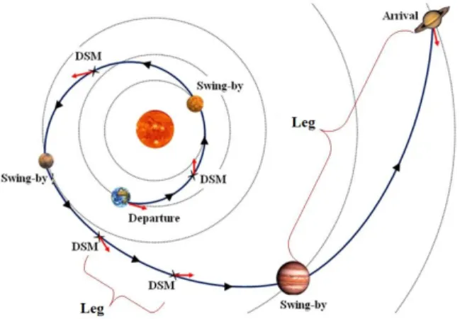
of design variables to be optimized is a variable). Consider, for example, the opti-mization of a space interplanetary trajectory. The spacecraft travels from the home planet to the target planet and it is desired to utilize the minimum fuel possible. As can be seen in Figure 1.1, the spacecraft can apply Deep Space Maneuvers (DSMs) which are propulsive impulses used to change the velocity of the spacecraft instanta-neously; these DSMs consume fuel proportional to the amount of the DSMs impulse. The spacecraft can also benefit from free change in momentum, through as many as needed flybys of other planets. When the spacecraft performs a flyby maneuver, we need to determine the height of closest approach to the flyby planet as well as the plane of the flyby maneuver. Hence, by changing the number of flybys the total number of variables change.
Figure 1.1: Interplanetary Trajectory Optimization Problem Topology
Besides the flyby planets, the spacecraft can have DSMs in any segment between any two planets. These segments are referred to as legs. The architecture of a solution
the mission architecture, the number of flybys, the planets of flybys, and the number of DSMs in each leg need to be optimized. These are called the architecture Other non architecture variables include launch and arrival dates, dates and times of flybys, dates and times of DSMs, amounts and directions of DSMs impulses. This is a VSDS optimization problem.
Another example is the optimization of a microgrid system where there are several energy sources and co-located energy storage devices that can either sink or source power with their corresponding sources. The net power at each source/storage is metered to the grid main bus using a boost converter. For an efficient design of the microgrid, the number of storage elements (N) and their capacities need to be opti-mized. Storage is expensive and designing a microgrid, with storage sized properly, is an open problem. Associated with computing the optimal N is the optimal values for the duty ratios at the converters that controls the power metered to the main bus from each source. A more complex situation is when we have M microgrids that have the ability to interconnect. This provides a large number of permutations for exchanging power. Systems design optimization problems are usually replete with local minima. Hence a global search algorithm is usually needed for optimizing the system variables, such as genetic algorithms (GAs) [10], particle swarm optimization [11], ant colony optimization [12], or differential evolution [13]. In VSDS optimization, the problem
can be formulated as follows: Minimize f(~x, N) Subject to ~g(~x)≤0, ~h(x~) =0, ~xl≤~x≤~xu (1.1) where ~x = [x1, x2, ..., xN] T
, N is the number of design variables, ~xu and ~xl are the upper and lower bounds of the variables~x, respectively. The number of variables N
in this formulation is variable, and its value dictates the architecture of the solution. The number of inequality constraints ~g and the number of equality constraints ~h, each is also a variable.
1.2
Genetic Algorithms
The research on developing algorithms that can handle VSDS optimization problems (sometimes referred to as variable length optimization) has started since about two decades. Standard GAs are not suitable for VSDS problems because they are designed to work only on problems of fixed number of variables. In standard GAs, the variables of the optimization problem are coded in chromosomes. Each chromosome represents a solution and consists of the variables that are coded as genes. In standard GA, the number of variables is assumed fixed and therefore, the number of the genes and the length of the chromosomes are fixed. By applying the evolutionary operations of
selection, mutation, and crossover, the population of these chromosomes converges to the global optimal solution [10]. The objective of optimization determines the fitness of the solution. The genetic operations of selection, mutation and crossover are applied on a population of these chromosomes, and through generations (iterations), theses populations converge to the optimal solution.
In the selection operation, two chromosomes are selected as parents from the gen-eration pool. In general, the chromosomes that have better fitness values (objective function), have higher probability to be selected as parents. After the parents are selected, mutation and crossover operations are applied on them. As an example, in binary coding, genes are coded as 0s and 1s; in the mutation process gene 1 may change to 0 with a probability ofpm. In the crossover operation, parts of the
chromo-some strings are swapped in parents. For example, in single point crossover, a random point is selected in both parents and the genes of one side of that point are swapped in parents with a crossover probability of pc to create new chromosomes. Some of
the best chromosomes (elites) are transferred to the next generation with no change. By repeating the GA operations in each generation, the population converges to the optimal solution.
Some variations of GAs have been proposed for VSDS problems. Genetic program-ming is a specialization of genetic algorithm in which each individual is a computer program [14, 15]. In genetic programming, the solutions are in the structure of trees
that can have variable lengths. A VSDS GA is presented in [16] in which a random operator is introduced to change the chromosome length, for the problem of Kauffman NK model. This random operator depends on the identity of genes which is given by their position relative to one end of the genotype. Reference [17] is a continuing work of [16] and analyzes the optimal location for the crossover point in VSDS problems. When two parents have different chromosome lengths, and given a selection for the crossover point in parent 1, reference [17] suggests that the crossover point in parent 2 be chosen such that the difference between the swapped segments is minimized. The method proposed in [17] is a search on all the possible crossover points in parent 2 to find the best cutoff point. The VSDS GA in reference [18] uses a two-point crossover, with different cutoff points in each parent, resulting in different lengths of the children chromosomes. This method is most useful in problems with variables of the same identity, like angles of a polyhedral where adding or removing one angle will result in a new polyhedral (e.g. triangle to rectangle or vice versa).
Reference [19] presents a number of variable length representation evolutionary al-gorithms that improves the sampling of a VSDS, with application in evolutionary electronics. In reference [20], the number of different chromosome lengths is set a priori, and both parents have the same crossover point (same gene index of cutoff). Therefore the length of the chromosome is switched from parents to children in [20] (the length of child 2 is equal to length of parent 1 and length of child 1 is equal to
length of a solution. A different approach in VSDS GA is to have equal-length chro-mosomes in each generation, yet the chromosome length is allowed to change among different generations as presented in [21, 22]. In this method, the GA starts with short-length chromosomes and the best solution in a generation is transferred to the next generation with a longer chromosome length. In this way, the GA handles fixed-size chromosomes in each generation, and there is no need to define new evolutionary operations for GA.
A structured chromosome genetic algorithm was developed in [23, 24] where the stan-dard one layer chromosome is replaced with a multi-layer chromosome for coding the variables; the number of genes in one layer is dictated by the values of some of the genes in the upper layers. Hence, it was possible to code solutions of different architec-tures. Yet, this structured-chromosome approach introduces new definitions for the crossover operation such that meaningful swapping between chromosomes of different layers is guaranteed. Some other algorithms are designed for specific problems. For instance, references [25] and [26] present tailored algorithms that search for the opti-mal structural topology in truss and frame structures, respectively. The dissertation in [27] presents a study on topology optimization of nanophotonic devices and makes a comparison between the homogenization method [28] and genetic algorithms [10]. As can be seen from the above discussion, many of the VSDS optimization algorithms are problem specific. The dynamic-size multiple population genetic algorithm has a high computational cost [29].
1.3
Space Trajectory Optimization
Space trajectory optimization is the process of searching for the optimal trajectory from one celestial body or orbit to another, such that the mission requirements are satisfied and a given objective is optimized. The objective can be minimizing the mission cost or fuel consumption, minimizing the mission duration, maximizing the number of visited asteroids, or a combination of these objectives. The spacecraft can have continuous or impulsive thrusters, for which various trajectory design tech-niques have been developed. In this dissertation, the impulsive thrust spacecraft is considered. The earliest research on space trajectory optimization goes back to the work of Walter Hohmann on trajectory design of a spacecraft with impulsive thrusters between two coplanar orbits [30]. Cornelisse [31] showed that in the patched conics method, the cost of an interplanetary trajectory mission can be reduced by applying a DSM. Several works have studied the effect of DSMs in different space missions [32, 33, 34, 35]. Planetary flybys utilize the gravity of a planet to change the mo-mentum vector of a spacecraft. Such trajectories that use DSMs and flybys are called Multi Gravity-Assist Deep Space Maneuver (MGADSM) trajectories.
To design a MGADSM interplanetary trajectory, many variables should be optimized depending on the mission type, such as launch and arrival dates and times, number of
flybys, planets to flyby, number of DSMs, epoch of each DSM, direction and magni-tude of each DSM, time of flight (TOF) between each two successive celestial bodies (leg), and flyby altitudes and rotation angles. These variables can be categorized into two groups of discrete design variables and continuous design variables, as shown in
Table 1.1. Since some variables are related to others (e.g. flyby attitude depends on whether there is a flyby or not), the problem can be considered as VSDS problem, in which the number of optimization variables vary among different trajectory mis-sions. In other words, the number of flybys and DSMs are not known a priori and they determine the number of other variables needed to model the problem. These variables that determine the total number of variables in a solution are referred to as the architecture variables.
Table 1.1
Design variables in an interplanetary trajectory optimization problem
Discrete Variables Continuous Variables Number of flybys (m) Departure date (td)
Flyby planets (P) Arrival date (ta)
Number of DSMs in each leg (n)
TOF
Flyby pericenter altitude (hp)
Flyby rotation angles (η) DSMs epoch ()
DSMs magnitudes and di-rections
problems, including heuristic algorithms [36, 37, 38, 39, 40, 41], deterministic algo-rithms [42, 43, 44], or a combination of them [45, 46]. Deterministic methods use grid or tree search to explore the design space. Although these methods converge globally, they can be extremely exhaustive, especially in complex missions with high number of flybys/rendezvous and DSMs or large time windows. The obtained solu-tions also are usually sensitive to the grid size. Heuristic methods on the other hand do not need discretization of the search space and are more adaptive and hence are not usually exhaustive. Yet they rely on heuristics and parameters tuning. Genetic algorithms (GAs) [47, 48, 49, 50, 51], differential evolution [41, 52, 53, 54], and ant colony optimization [55] are some of the heuristic algorithms that have been used in MGADSM optimization problems.
In MGADSM problems, since in general the flyby and DSM structures are not known a priori, it is not possible to use the standard GAs without simplifications on the problem or modification to the algorithms [36, 56, 57]. One way of simplifying the problem is to prune the state space (assume fixed flyby sequence and number of DSMs) to limit the possible mission scenarios. A deterministic search is used in [57, 58] where the flyby sequence and DSMs are fixed and the search space is limited to a grid of points where the global optimization methods can be used. Another way of simplifying the problem is to use a nested loop solver to optimize the trajectory [37, 59]. The outer loop finds the optimal flyby sequence and the inner loop optimizes
of flybys, this problem is a VSDS optimization. Early methods pruned the outer loop to solutions that the designer considered to include the optimal flyby sequence [60]. Later, automatic methods were proposed to find the flyby sequence in MGA trajectories. Some graphical methods use the energy contours against two variables that define the orbits for different planet flybys [61, 62]. This method can be used when all the flybys are considered non-powered and it is assumed that there is no DSMs. In [59] a maximum length for the flyby sequence is assumed and the outer loop is optimized using a binary genetic algorithm. By adding null variables that represents a ”no flyby”, variable-sized flyby sequences can be modeled in this method. For example, for a maximum flyby of two, the Earth-Venus-Mars (EVM) sequence is equivalent to a mission from Earth to Mars with a flyby around Venus and a null flyby that is not considered in the cost function. Genetic algorithm is also used for multiple phase maneuvers where there is both impulsive and continuous maneuvers [37]. Genetic Programming [15] is also among the earliest approaches that addressed the VSDS optimization problems. One of the earliest attempts in implementing gene expression in GA is to perform “cut and splice” on the chromosomes and applying a self adaptive recombination operator on them to yield individuals of variable lengths [63, 64]. In recent years, the role of histone in the regulation of DNA including gene expression and functionality of each cell was discovered [65], which resulted in the use of epigenetics through modification of histone in strongly-typed genetic programming [66]. A dynamic-size multiple population genetic algorithm was developed in [29]
where each generation consists of a number of sub-populations; all chromosomes in each sub-population are of the same length. Hence each sub-population evolves over subsequent generations as in a standard GA. The size of each sub-population, however, changes dynamically over subsequent generations such that more fit sub-populations are allowed to increase in size whereas lower fit sub-sub-populations decreases in size. This approach has been applied to the trajectory optimization problem and demonstrated success in finding best know solution architectures. The computational cost of this method, however, is relatively high since it implements GA over several sub-populations in parallel. Also, only a finite number of architectures (assumed a priori) can be investigated using the method in [29].
1.4
Motivations and Objectives
Inspired by the concept of gene expression in biology, the concept of Hidden Genes Genetic Algorithm (HGGA) was introduced to search for the optimal architecture and autonomously generate new design spaces [2, 3]. Reference [3] applied a simplified version of the HGGA for interplanetary trajectory optimization and demonstrated success in finding the best known solution architectures for known benchmark prob-lems. This original version of the HGGA implemented in [3] assumes a long chromo-some for each solution where chromo-some of the genes are hidden. In this version, genes in a
Hence, the HGGA will not attempt to hide genes if the chromosome is a feasible solution. Therefore, this developed method of HGGA lacks a rigorous mechanism for selecting the hidden genes in each generation.
In this dissertation, the objective is to develop new mechanisms for hiding genes. These mechanisms should have the following properties:
1. They should autonomously decide which genes should be hidden.
2. They should not be problem specific; i.e. they should be applicable to any VSDS problem with no modification of the algorithm in any kind or simplifi-cation on the problem. The problems can be constrained or non-constrained, discontinuous, non-differentiable, stochastic, or highly nonlinear.
3. They must promise convergent solutions.
4. They should produce comparable results to other algorithms for VSDS prob-lems.
Note that the proposed algorithms in this dissertation are stochastic optimization algorithms. Hence, there is no guarantee that the solutions found with these al-gorithms are global optima. In this dissertation however, the results found by the designed algorithms are referred to as the optimal points/solutions.
1.5
Organization of the Dissertation
This dissertation consists of six chapters covering the objectives described in the previous section. In preparing this dissertation, the materials of papers written during this research are utilized. Chapter 2 covers the necessary background material on GAs and HGGAs. The concept of HGGAs in biology is explained and the original feasibility criteria for HGGAs is described. Chapter 3 is focused on developing new HGGA mechanisms. The concept of tags and alleles in HGGAs are presented and several stochastic and deterministic evolution mechanisms of the tags and alleles are proposed. In Chapter4, the performance of these mechanisms are tested on various VSDS problems, including mathematical problems and space trajectory optimization problems. InChapter5, the Markov Chain convergence analyses of the HGGAs with the proposed mechanisms are performed and finally the conclusion of the dissertation is presented in Chapter 6.
Chapter 2
Hidden Genes Genetic Algorithms
2.1
Introduction
In this chapter 1, the concept HGGAs is presented. To handle a VSDS (or
architec-ture) optimization problem, the idea of turning genes on and off was adapted from biology in genetic algorithm. By setting the chromosome length equal to the length of the longest possible chromosomeLmax (maximum number of design variables) and
turning some genes off, different solutions (of different architectures) with lengths of 1 to Lmax can be built while having the same length for all the chromosomes.
More-over, having similar lengths for all the chromosomes enables the implementation of the standard GA operations like crossover and mutation on them. The genes that are 1The material of this chapter are copied in part from References [4, 6, 7]
hidden are variables that do not affect the fitness of the solution; yet they carry in-formation, go through GA operations, and may become active (not hidden) in future generations. In the next section, the equivalent of HGGAs in biology is explained and an initial hidden genes assignment mechanism is described.
2.2
Modeling Genes and Chromosomes
In standard GAs, the mechanics of natural selection and genetics are simulated [10]. For each solution a chromosome is considered which is a set of coded variables called genes. Figure2.1 shows a typical chromosome that consists ofN genesg1, g2, . . . , gN.
The value of gi determines the value of that variable in that solution. The fitness of
the solution is determined based on the objective of optimization.
Figure 2.1: In standard GA, a chromosome (code) is a string of genes that represent a solution
The algorithm starts by applying the genetic operations of selection, crossover, and mutation on a population of these chromosomes. Through generations (iterations), this population converges to optimal solutions. In the selection operation, the chro-mosomes that are more fit, have higher probability of being selected as parents. After parents are selected, the crossover and mutation operations are applied on them to
create new children chromosomes. For example, in the single point crossover, a ran-dom point in parents strings is selected and the gene strings of both sides of that point are swapped in parents to create new individuals. The crossover probability of
pc is applied to the crossover operation to make sure that the fit individuals found in
the previous population survive without modification. In the mutation operator, each gene is mutated with probability of pm. For example, in binary coding, gene 0 may
change to 1 through mutation operator. By repeating the selection, crossover, and mutation operations in each generation, the population converges to a (near) optimal solution.
2.3
Hidden Genes in Biology
In genetics, the deoxyribonucleic acid (DNA) is organized into long structures called chromosomes. Contained in the DNA are segments called genes. Each gene is an instruction for making a protein. These genes are written in a specific language. This language has only three-letter words, and the alphabet is only four letters. Hence, the total number of words is 64. The difference between any two persons is essentially because of the difference in the instructions written with these 64 words. Genes make proteins according to these words. Since, not all proteins are made in every cell, not every gene is read in every cell. For example, an eye cell doesn’t need any breathing genes on. And so they are shut off in the eye. Seeing genes are also shut
Figure 2.2: Chemical tags (purple diamonds) and the ”tails” of histone proteins (purple triangles) mark DNA to determine which genes will be tran-scribed. (picture is modified from [1])
off in the lungs. Another layer of coding tells what genes a cell should read and what genes should be hidden from the cell [67]. A gene that is being hidden, will not be transcribed in the cell. There are several ways to hide genes from the cell. One way is to cover up the start of a gene by chemical groups that get stuck to the DNA. In another way, a cell makes a protein that marks the genes to be read; Figure 2.2 is an illustration for this concept. Some of the DNA in a cell is usually wrapped around nucleosomes but lots of DNA are not. The locations of the nucleosomes can control which genes get used in a cell and which are hidden [67].
2.4
Concept of HGGAs in Optimization
The concept of Hidden genes is applied in GA to make some genes hidden (inactive), so that their value does not affect the fitness of objective function. The genes that are hidden are variables that should not appear in a specific solution. This concept allows GA to be able to handle VSDS and architecture optimization problems. In such problems, the number of design variables is variable and the length of the chromosome changes by selecting different values for some of the design variables. LetLmax be the
length of the longest possible chromosome (maximum number of design variables). In hidden gene concept, all the solutions (chromosomes) have the same length and hence the operators of standard GA can be applied to them. Genes that are hidden will be ineffective in fitness of the objective function, although they take part in the genetic operations in generating future generations.
Figure 2.3: Hidden genes and effective genes in two different chromosomes [2]
Consider two chromosome with different lengths. Assume that there are four genes in the first chromosome and three genes in the second chromosome (represented by bi-nary bits inFigure2.3). Also assume that the maximum number of genes (variables) in a chromosome is six. To make this problem a fixed-sized design space problem, two hidden genes are added to the first chromosome, and three hidden genes are added to the second chromosome. These added genes are hidden and therefore do not affect the fitness of the objective function. Since all the chromosome have the same length now, the standard GA operators can be applied to them. These added (hidden) genes go through crossover and mutation like active genes. Based on the mechanism that assign the hidden genes, a hidden gene in parents can be active in children (and hence effective in fitness evaluation).
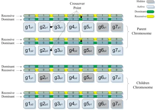
A simple example of a single-point crossover operator in HGGA is shown in Figure
2.4. In this figure, the crossover point is between the second and third genes. After the genes are swapped, the location of hidden genes in children may be similar to or different than the hidden genes in the parents. The genes that should be hidden are selected based on a specific hidden gene assignment method. In the initial studies on HGGA [2, 3], a primitive mechanism (calledfeasibility mechanism”) was introduced.
In these works, the hiding criteria was feasibility, meaning that the genes were all active unless the solution was infeasible. In that case, the genes would be hidden one by one until a feasible solution is achieved.
Figure 2.4: Crossover operation in HGGA [2]
2.5
Conclusion
The concept of hidden genes and their equivalent in biology were introduced in this chapter. To determine the status of genes, the feasibility mechanism can be utilized where genes are hidden one by one from one side of the chromosome until a feasible solution is acquired. However, this mechanism is not robust specially when variables are simulated in various locations of the chromosome as genes. In the next chapter, new mechanisms are proposed for hiding gens. In these mechanisms, the status of the genes can evolve through generations while the genes are evolving.
Chapter 3
Hidden Genes Assignment
Methods
3.1
Introduction
In this chapter1, new mechanisms are proposed to hide genes. The concept of tags is
described and eight stochastic mechanisms with tags, three logical mechanisms, and the concept of alleles are presented. In the logical mechanisms, the logical OR and
OR operators are used. For x and y expressions, the logical OR operator is true if
either ofxoryare true. The logical AND operator results in true if xandyare true.
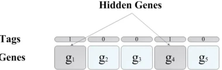
As described in Section 2, the protein of each gene makes it to be read or hidden. This gave us the idea to use tags for genes to make them hidden or active. To code such tags, binary digits of 0 and 1 are assigned to each tag, as shown in Figure 3.1. If the value of tagi is 1, then the corresponding gene xi is hidden, and if it is 0, gene
xi is not hidden (active).
Figure 3.1: HGGA and the tags concept
Chromosomes evolve over successive generations. Genes along with their tags go through evolutionary operations. Genes evolve through the standard operations de-fined in the CGA. The tags, however, may evolve with different operations. A set of operations used to evolve tags is here referred to as a mechanism for tags’ evolution.
3.2
HGGAs Mechanisms
There are 12 different mechanisms for tags evolution that will be investigated in this section. In the mechanisms that have a crossover operator for the tags, the singe-point crossover is used, unless otherwise stated. Some of the evolution mechanisms are logical. Here we introduce two definitions. Consider two parents selected for
reproduction and consider one offspring child. The Hidden-OR evolution logic is defined as follows: a gene in the child chromosome is hidden if the same gene is hidden in any of the parents. The Active-OR evolution logic is defined as: a gene is active in the child if the same gene is active in any of the parents.
1. Mechanism A: tags evolve using a crossover operator. The crossover point location in the tags can be different from that in the genes. Before the crossover, tags go through a mutation with probability of 10%.
Figure 3.2: Schematic of Mechanism A
2. Mechanism B: When two parents are selected for reproduction, then the process of evolving the tags is as follows:
i - produce two temporary children through a single-point crossover opera-tion on genes, and an Active-OR logic on tags. Both of these temporary children will have the same tags.
iii - consider the parents chromosomes (genes and tags) as points in IRL+Lt space whereLt is the number of tags.
iv - the child (output of Mechanism B) is the weighted arithmetic crossover on the parents and is closer to the parent that has better fitness ¯f for its temporary child.
For example, for the IR3 space in Figure 3.3, the child is closer to parent 1
because its temporary child has better fitness value. λ is a random number in (0,0.5). If ¯f1 = ¯f2, then the child can be randomly closer to either parents.
Figure 3.3: Representation of arithmetic crossover in IR3.
In this mechanism, the mutation operator is only allied to the genes.
3. Mechanism C: The arithmetic crossover operator is used for the genes only. The tags in the child will have the same tags of one of the parents depending on the value of fm1 =f+
PLt
i=1tagi
, where f is the fitness of the parent. The offspring tags will be the same as that of the parent that has better value of
Figure 3.4: Schematic of Mechanism B.
of hidden genes.
4. Mechanism D: same as Mechanism C, but the offspring tags have the same values as that of the parent with better value of fm2 =f −
PLt
i=1tagi
. In other words, this mechanism favors less number of hidden genes.
5. Mechanism E: tags evolve only through a mutation operation with a certain mutation probability different than the mutation probability of the genes. So, two parents are selected; then mutation for the genes is carried out and another mutation for the tags is carried out. These two parents then go through a crossover operation on the genes with a certain probability as in the CGA, while the tags remain unchanged during this crossover operation.
6. Mechanism F: tags are considered as discrete variables where they are appended to the genes to create a long chromosome that has both genes and tags. Then the mutation and crossover operations are carried out in a similar way to that of the CGA.
7. Mechanism G: this mechanism is similar to Mechanism F except that the tags do not go through a mutation operation.
8. Mechanism H: this mechanism is similar to Mechanism F except that the tags do not go through a crossover operation. This is carried out by limiting the crossover point to be within the genes only.
9. Alleles: in biology, an allele is an alternative form of a gene and in human cells, there are two alleles of a gene in each position on a chromosome, one dominant and one recessive. Dominant traits are expressed only when the alleles of a pair are heterozygous (the individual only has one copy of the allele). For example, the allele for brown eyes is dominant, meaning that there is only one allele of brown eyes needed to have brown eyes. On the other hand, the recessive traits are expressed only if the alleles of a pair are homozygous (the individual has two copies of the allele). These principles and their traits was first discovered by Gregor Mendel [68, 69] and is named as Mendel’s Law of Segregation. Knowing this concept in biology, two sets of tags (alleles) are considered for genes in HGGA, in which only the dominant allele decides whether a gene is hidden or active but both dominant and recessive alleles go through GA operations and affect the next generation’s status. Therefore a recessive allele in the current generation may become a dominant allele in the next generation. For the evo-lution process, the mutation operation is first carried out in the genes and tags.
crossover operator is applied to the tags such that the crossover point in the dominant and recessive tags are similar.
Figure 3.5: Schematic of Alleles Mechanism.
10. Logic A: the member of the current generation (¯n) is split into two groups of equal size. For the first group, the Active-OR logic is used for tags evolution (a gene is active in the child if the same gene is active in any of the parents). For the second group, the Hidden-OR logic is used for tags evolution (a gene is hidden in the child if the same gene is hidden in any of the parents).
11. Logic B: similar to Logic A; but the Hidden-OR logic is used for all the members in the generation.
Figure 3.6: Schematic of Logic A.
Figure 3.7: Schematic of Logic B.
Figure 3.8: Schematic of Logic C.
3.3
Conclusion
In this chapter, the concept of binary tags was introduced in genetic algorithms to enable hiding some of the genes in a chromosome, so that they can be used to search for optimal architectures in VSDS problems. The proposed binary tags concept mimics biological cells in hiding the genes that are not supposed to be effective in the cell, while they could be effective in other cells. Various mechanisms for assigning the chromosome hidden genes were proposed and investigated in this chapter. These mechanisms make assigning the status of the genes more robust compared to the feasibility criteria and can be applied to any problem with various number of hidden genes for different types of variables. By evolving tags through generations, the status of the genes evolve at the same time that their values evolve. This extended
functionality in HGGAs is robust and easy to implement. All the mechanisms are tested on different VSDS problems in the following chapter.
Chapter 4
Test Cases
4.1
Introduction
In this chapter1, the proposed mechanisms are tested on two types of VSDS problems.
The first type is mathematical problems that are used as the primary performance evaluation for the mechanisms. Their performance is compared to the initial concept of HGGAs (feasibility criteria). After that, the mechanisms are tested on three space trajectory optimization problems. These problems have different levels of complexity and are adapted from the standard space trajectory optimization benchmark. The performance of the mechanisms are compared and their capabilities are evaluated.
4.2
VSDS Mathematical Functions
Multi-minima mathematical functions can be very useful in testing new optimization algorithms. However, there is not many multi-minima VSDS mathematical func-tions in the known benchmark mathematical optimization problems. Four benchmark mathematical optimization problems were modified to make them VSDS functions; and then they were used to test the new HGGA mechanisms. These functions are: the Egg Holder, the Schwefel 2.26, and the Styblinski-Tang functions. These functions and their variable ranges are as follows [70]:
1. Egg Holder: continuous, differentiable, and multimodal.
FEG(X) = N X i=1 (−(xi+1+ 47)sin( p |xi+1+xi/2 + 47|)− xisin( p |xi−(xi+1+ 47)|)), −512≤xi ≤512 (4.1)
2. Schwefel 2.26: continuous, differentiable, and multimodal.
3. Styblinski-Tang: continuous, differentiable, and multimodal. FSch(X) = 1 2 N X i=1 (x4i −16x2i + 5xi), −5≤xi ≤5 (4.3)
The general concept of modifying these functions to be VSDS functions is here de-scribed. Consider the optimization cost function defined as:
F(X) =
N
X
i=1
fi (4.4)
If tagi is 1 (hidden), then fi is set to zero. In other words, if a variable (gene) i is
hidden, then the correspondingfi is zero, or does not exist. This is consistent with the
physical systems test cases presented inSection1.1. Unlike the tags, the genes evolve through the standard GA selection, mutation and crossover operations. In general, standard GA are not suitable for solving VSDS problems. However, a significant advantage of using the above modified mathematical functions is the possibility of using standard GA if we assume all variable are active (not hidden). If the optimal solution has xj hidden ∀j ∈ Γ, and Γ ⊆ {1,2,· · · , N}, then the standard GA can
find that optimal solution, if we assume all variables are not hidden. In such case, the optimal solution that the standard GA would search for is x∗j where f(x∗j) = 0, ∀j ∈Γ.
functions. For the genes, a single point crossover and an adaptive feasible mutation operators are selected. The GA parameters used in these simulations are listed in
Table 4.1.
Table 4.1
Genetic Algorithm Options
Option V alue Population Size 400 Number of Generation 300 Elite Count 20 StallGenLimit Count 25 Crossover Fraction 0.95 TolFun 1e−6
where Elite Count is the number of solutions that go to the next generation
with-out any change and the algorithms stops if the average relative change of the best solution over StallGenLimit generations is less than or equal to TolFun. Note that the crossover fraction in Table 4.1 is for the genes and the tags evolve based on the characteristics of each mechanism. In Equation 4.4, if fi is a function of xi only,
there are N tags, and if fi is a function of xi and xi+1, then there are N −1 tags.
In all the problems, the number of variables without tags is 5. Each test case is simulated 20 times. Superior, a high-performance computing cluster at the Michigan Technological University, was used in obtaining the results presented in this section. This computing cluster is Generation 2 with 47 CPU compute nodes, each having 32 CPU cores (Intel XeonE5−26832.10 GHz) and 256 GB RAM2. The best solutions,
average, variance, computational time (in seconds), average number of generations until convergence, and success rate of 20 simulations are presented in Table 4.2-4.4. The problems are also solved with the initial concept of HGGAs presented in [2]. The results show that Mechanisms A and G, Logic A and G, and alleles concept have better overall performance compared to others. Moreover, based on the overall results presented in Table 4.2-4.4, the Egg Holder function seems to be the most difficult problem among the three chosen problems with higher variance and variation in the best solution found. In the Egg Holder function, all the proposed mechanisms except Mechanism B, C, and D could find solutions with lower cost value compared to the initial HGGA concept. In the Schwefel 2.26 and Styblinski-Tang functions, several mechanisms could find solutions with similar or close cost value to the solution of ini-tial HGGA concept. Although the computational time of the iniini-tial HGGA concept is lower for both test functions. However in the Schwefel 2.26 function, the success rate of the alleles concept is higher than the initial HGGA concept with the same cost value as the best solution. In the Styblinski-Tang function, the best solution among the tested mechanisms has a cost value of −195.8308 and most of the mechanisms
are able to find close solutions to that with high success rate. Mechanisms B, C, D, and Logic B have the highest cost (not desired) and lowest success rate in all the problem. However, this is expected for Logic B since it favors solutions with more hidden genes. In the tested problem however the best solution is to have all the genes active and therefore the performance of Logic B is not good. Regardless, in problems
where the optimal solution has some hidden and some active genes, Logic B might have better performance. The success rate of the Egg Holder function is shown in Figure 4.1 as an example. On each of these boxes, the
Figure 4.1: Success rate of some mechanisms in Egg Holder function.
By repeating the same numerical experiment, the obtained solution in each experi-ment is compared to the best obtained solution and a success rate can be updated as the experiment being repeated. A success rate of 0.3 means that if the simulations are repeated ten times, it is expected that three simulations have a cost value of around 95% of the best solution found overall. The box diagram of the mechanisms for the Egg-Holder function is shown in Figure 4.2. In this figure, A through H refer to mechanisms A through mechanism H, and LA, LB, and LC refer to logic A, logic B, and logic C, respectively. On each box, the central red mark is the median, the
dotted black line is the data considered in the calculations, and the red ‘+’ symbols are the outliers.
Figure 4.2: Box diagram of all the mechanisms in Egg Holder function.
The results of this section give more insight on the performance of the proposed HGGA mechanisms and can be used as an initial statistical analysis. The mechanisms showed potential for more investigation and hence, in the next section they are tested on space trajectory optimization problems.
Table 4.2
Egg Holder function results
Mechanism Best Average Variance Tc Ng SR
Logic A −3674.8391 −3330.7773 55850.2062 191.1277 242.25 30 Logic B −3010.1431 −1992.4732 127557.2779 176.4492 222 5 Logic C −3636.4812 −3351.7976 38493.6971 170.9710 215.55 30 Mechanism A −3627.2132 −3191.2960 39502.0731 121.9006 140.5 20 Mechanism B −2282.3187 −1665.2146 70489.6712 67.1561 45.1 5 Mechanism C −2445.1901 −1785.3663 109847.1527 67.6609 47.95 5 Mechanism D −2521.0772 −1736.6389 85834.8496 63.9779 45.2 5 Mechanism E −3607.1362 −3014.7806 72811.4486 71.2453 77.65 5 Mechanism F −3592.4893 −3249.7519 56730.4356 210.2351 285.55 20 Mechanism G −3679.5732 −3276.8970 56740.0155 185.6655 250.85 25 Mechanism H −3455.9918 −3097.3507 34409.3814 220.8240 281.8 20 Alleles −3664.1354 −3377.8405 46136.7272 644.6538 233.35 35 Initial HGGA −2808.1814 −2496.6042 45111.6674 111.7339 127.8 30 Table 4.3
Schwefel 2.26 function results
Mechanism Best Average Variance Tc Ng SR
Logic A −418.9828 −417.6561 28.1062 116.1333 141.35 95 Logic B −335.1862 −258.0072 963.0126 165.8180 208.55 5 Logic C −418.9828 −418.8164 0.4639 105.3200 127.8 100 Mechanism A −418.7245 −410.5598 67.1025 74.5818 78.65 85 Mechanism B −263.7859 −223.3435 600.5483 74.6767 50.95 10 Mechanism C −350.4428 −251.4763 1722.6184 80.2498 59 10 Mechanism D −286.7516 −233.8988 868.0824 76.9453 57.15 10 Mechanism E −418.2302 −394.9007 517.0262 57.4893 60.7 55 Mechanism F −418.9828 −417.2749 28.2410 191.4418 256.2 95 Mechanism G −418.9828 −416.0680 38.4820 140.2377 188.65 95 Mechanism H −418.8752 −401.3159 310.9379 204.2924 267.95 50 Alleles −418.9829 −418.9218 0.07207 369.3322 132.4 100 Initial HGGA −418.9829 −416.6141 53.1574 63.0096 67.05 90
Table 4.4
Styblinski-Tang function results
Mechanism Best Average Variance Tc Ng SR
Logic A −195.8307 −195.8281 0.00011 74.4599 84.95 100 Logic B −195.8307 −155.7955 386.6748 97.8044 115.6 10 Logic C −195.8308 −195.8302 1.3061e−06 71.8116 80.85 100 Mechanism A −195.8304 −195.7179 0.04677 98.74251 107.65 100 Mechanism B −176.0926 −158.9485 172.4940 99.1229 70.4 35 Mechanism C −190.5350 −165.1095 185.9181 90.3370 67.2 15 Mechanism D −189.2275 −164.6126 151.5187 86.1996 63.35 5 Mechanism E −195.8097 −188.1418 137.0943 74.4072 83.2 70 Mechanism F −195.8307 −195.8301 6.7591e−07 75.6282 91.9 100 Mechanism G −195.8308 −195.8304 2.4139e−07 75.3374 91.7 100 Mechanism H −195.8308 −195.1230 9.9912 84.8920 98.5 95 Alleles −195.8308 −195.8301 6.4460e−07 246.5077 83.35 100 Initial HGGA −195.8308 −195.8308 1.4025e−15 49.8379 50.95 100
4.3
Space Trajectory Optimization
The purpose of interplanetary trajectory design is to select different variables such that a spacecraft travels from of celestial body to another with the best objective function. To get to the final destination, the spacecraft can have multiple revolu-tions around the sun, different flybys around other celestial bodies, and also multiple DSMs in each leg. The number of flybys and DSMs are the variables that describe the topology of the mission and make the problems a VSDS optimization problem. Other variables of this problem include the launch and arrival time, flight direction, time of flight for each leg, pericenter altitude for each flyby, rotation angles, epochs of DSMs, and the DSM vectors (direction and magnitude). These variables can be cat-egorized into two groups of discrete design variables and continuous design variables
(Table 4.5).
Table 4.5
Design variables in an interplanetary trajectory optimization problem
Discrete Variables Continuous Variables Number of flybys (m) Departure date (td)
Flyby planets (P) Arrival date (ta)
Number of DSMs in each leg (n)
TOF
Flight direction (fdir) Flyby pericenter altitude
(hp)
Flyby rotation angles (η) DSMs epoch ()
DSMs magnitudes and di-rections
It is assumed in this study that the spacecraft operates with impulsive thrust and can have multiple DSMs in each leg. The objective function is to minimize the fuel consumption, which can be divided into departure (launch) impulse, arrival impulse, and DSMs maneuvers. ∆vtot =||∆Vd||+||∆Va||+ n X i=1 ||∆VDSM||+ m X i=1 ||∆Vps|| (4.5)
where ||∆Vd|| is the launch impulse, ||∆Va|| is the arrival impulse, n is the total
number of DSM maneuvers, m is the number of powered gravity assist maneuvers, ||Pn
i=1∆VDSM|| is the total costs of DSM maneuvers, and
Pm
i=1||∆Vps|| is the total
When there are no DSMs or flybys for a mission, the trajectory problem becomes a Lambert’s problem. Lambert’s problem is a two-body boundary value problem that computes the trajectory using initial and final heliocentric position vectors and TOF. The initial and final heliocentric positions of the spacecraft are assumed to be the same as the heliocentric position vector of the home planet and target planet at the initial and final time, respectively. The solution of the Lambert’s problem determines the departure and arrival impulses, and hence the transfer orbit.
In the case of an n-impulse trajectory with no flybys (n DSMs in one mission leg), the independent design variables are assumed the departure and arrival time, the ∆V
vector of n impulses, and the epoch of the DSMs. Knowing the departure time, the planet heliocentric position vector can be determined (assumed equal to the helio-centric position vector of the spacecraft). Since the epoch of the first DSM and the initial velocity vector are known, the Kepler’s equation can be used to propagate the position and velocity vector of the spacecraft at the DSM epoch. The velocity vector of the spacecraft after the DSM can be computed as the summation of the velocity vector of the spacecraft before the DSM and the DSM impulse vector. This procedure is repeated for all the transfer orbits of the trajectory except the last one, where the Lambert’s problem is solved. For the last transfer orbit, the arrival time and hence the orbit’s TOF are known. The planet’s position vector can be determined (equal to the spacecraft position vector at arrival) and therefore, the Lambert’s problem can be used. This results in the arrival impulse for capture by the planet.
Figure 4.3: Geometry of a non-powered flyby.
The spacecraft can have multiple powered or non-powered gravity-assist maneuvers (flybys). The momentum change in a flyby maneuver can impact the ∆V needed for the spacecraft during the mission. The spacecraft position vector during the flyby is assumed not to change and is equal to the heliocentric position vector of the planet at the flyby instance.
r− =r+=rp (4.6)
where r− and r+ are the position vectors of the spacecraft before and after the flyby
maneuver andrp is the heliocentric position vector of the planet at the flyby instance.
The velocity vector of the spacecraft after the flyby maneuver is determined by cal-culating the magnitude and direction of the velocity for powered and non-powered
† Non-powered flyby: It is assumed that during the flyby, the linear momentum
of the spacecraft changes only due to the gravity field of the planet. Hence, the magnitude of incoming and outgoing relative velocities are the same:
|v−∞|=|v+∞|=v∞ (4.7)
where v−∞ and v+∞ are the incoming and outgoing relative velocity vectors,
re-spectively and are calculated as:
v∞ =vS/C −vp (4.8)
vS/C is the spacecraft velocity vector and vp is the planet velocity vector
(Figure 4.3). The direction of the outgoing velocity can be determined by the flyby plane rotation angle δ.
sin(δ/2) = µp
µp +rperv2∞
(4.9)
where µp is the gravitational constant of the planet and rper is the pericenter
radius of the flyby which is a design variable. The maximum rotation angle is when the pericenter radius is minimum. If the required rotation angle is greater than the maximum achievable rotation angle, a powered flyby maneuver
is needed. The total spacecraft velocity change in a non-powered flyby is:
∆vnpf = 2v∞sin(δ/2) (4.10)
† Powered flyby: Higher rotation angles can be gained by applying a small impulse
during the flyby [71]. The spacecraft velocity on the periapsis trajectory (vm)
is [72]:
vm =
q
v2
∞+ 2µp/rper (4.11)
Hence, the required change in velocity for powered flyby is:
∆vpf =v+m−v − m = q v+ ∞2 + 2µp/rper− q v− ∞2+ 2µp/rper (4.12)
The outgoing velocity of the spacecraft in heliocentric inertial frame can be calculated as follows [3]:
v+∞=C(v+∞)L (4.13)
where (v+∞)Lis the outgoing relative velocity vector expressed in the local frame
ˆiˆjkˆ and C = [ˆi ˆj ˆk] is the transformation matrix between local frame and inertial frame. As shown in Figure 4.4, (v+
Figure 4.4: The local and inertial frames [3].
The local frame is defined such that ˆiis in the direction of the incoming relative velocity and ˆj is perpendicular to ˆi and is in the plane of the flyby maneuver. Line Γ in Figure 4.4 is the intersection of ˆjkˆ plane (Π plane) and the inertial Ecliptic plane ˆIJˆ. The angle between ˆI and Γ is Ω, and the angle between Γ and ˆj is η. Also, ι is the inclination of plane Π to the Ecliptic plane. By this nomenclature, the unit directions can be derived as [3]:
ˆi= v−∞ |v−
∞|
ˆ j = cos(−Ω) sin(−Ω) 0 −sin(−Ω) cos(−Ω) 0 0 0 1 × 1 0 0 0 cos(−ι) sin(−ι) 0 −sin(−ι) cos(−ι) × cos(−η) sin(−η) 0 −sin(−η) cos(−η) 0 0 0 1 1 0 0 (4.16) ˆ k = ˆi׈j (4.17)
For the full MGADSM problem withm flybys and ni DSMs in each leg (i= 1. . . m),
the calculations for each leg is carried out as explained above. Departure and arrival dates and the TOF of each leg (except the last leg) are design variables. The TOF of the last leg can be calculated knowing the total TOF of the mission and the summation of the TOF of the other legs. Assume that there aren1 DSMs in the first leg. Hence,
there are n1 + 1 transfer orbits in that leg. The calculations of the first nl orbits
are similar to the explanations on the n-impulse trajectory. For the last orbit, the velocity vector at the end point is the incoming heliocentric velocity of the flyby. The flyby is assumed non-powered if at least one DSM is in the following leg. Knowing the
(the spacecraft initial heliocentric velocity vector for the next leg) can be determined by carrying out the non-powered flyby calculations. This procedure is repeated for all the legs. In case of no DSMs in a leg, the initial flyby of that leg is assumed a powered flyby and the corresponding calculations can be used.
For all the problems, the J2 effect is ignored. Since Lambert’s problem can have multiple solutions, the maximum number of revolutions is set to 5 and the best solution from Lambert’s problem is selected as the trajectory for the current transfer orbit. The criteria to choose the best Lambert’s solution; i.e. choose the number of revolutions, is to select the one that results in the lowest segment cost. This cost can be the post-flyby maneuver, departure impulse, or a DSM impulse.
To illustrate how this problem is a VSDS optimization problem, two sample solutions are shown as chromosomes inFigure4.5. In this example, the hidden genes are shown with gray color. The top part of the figure shows the chromosomes in HGGA, with hidden genes and equal lengths, and the bottom part of the figure shows the equivalent chromosomes with no hidden genes and different lengths. As seen, depending on the number of flybys and DSMs, the length of the solutions can be variable. In the first solution, there is one flyby and one DSM, and in the second solution there are two flybys and two DSMs. Assume that it is required to send a spacecraft to planet Jupiter with the lowest cost (fuel consumption) within certain ranges for launch and arrival dates. The two solutions shown in Figure 4.5 can be interpreted as follows:
Figure 4.5: An example of two different solutions for an interplanetary trajectory problem in HGGA (Earth to Jupiter), and the equivalent chro-mosomes with no hidden genes in GA.
1. First Solution: A trajectory with one flyby around Venus (Earth-Venus-Jupiter) and one DSM in the second leg.
2. Second Solution: A trajectory with two flybys around Venus and Earth (Earth-Venus-Earth-Jupiter or EVEJ) and two DSMs in the first and the third legs.
This is a VSDS problem; the proposed tags/Alleles mechanisms can be used to search for the optimal solution and architecture.
In this study, three benchmark problems are investigated: Earth to Mars, Earth to Jupiter, and Earth to Saturn. The best known solutions for these problems can be found in the European Space Agency (ESA) website 3 and also in [3, 73].
The HGGA mechanisms are capable to search for the optimal variables including flyby sequences, DSMs’ epochs, magnitudes, and directions, launch and arrival dates, and flight direction. To reduce the computational cost, the problems are solved in two phases. In the first phase, the number of design variables is reduced by assuming that there are no DSMs (zero-DSM phase). Reducing the number of design variables in this phase allows for search in larger range of remaining variables. Hence, more planets can be explored for flyby sequence and wider launch, arrival, and flyby dates can be investigated. The second phase is a multi-gravity-assist with DSMs (MGADSM phase) that uses a fixed flyby sequence (obtained in the first step) to optimize the rest of the design variables including the DSMs in the mission. The range of launch, arrival, and flyby dates in the MGADSM phase are selected around the results of the zero-DSM phase. This approach has shown to be computationally efficient [3] compared to a single model where all the variables including DSMs and flyby sequences are optimized together. However, it should be kept in mind that in some missions (such as Messenger), solving the problem in two phases may result in exclusion of fit solutions. For example, some mission trajectories are only fit when there are DSMs and by removing the DSMs, they become unfit and hence get omitted from the zero-DSM phase. Therefore, the feasibility of optimizing the trajectory in two phases should be studied beforehand for each mission.
Each simulation is repeated 100 times for the purpose of statistical analysis on the http://www.esa.int/gsp/ACT/inf/projects/ gtop/cassini2.html, date retrieved: December 06, 2017
efficiency of the method. For all the problems, the elite count is 20, the crossover probability is 0.95, and the algorithms stops if the average relative change of the best solution over 25 generations is less than or equal to 10−6. The create function
for initial population is uniform, the selection function is roulette wheel. Single point crossover and adaptive feasible mutation functions are used for the genes. For the sake of comparison, the lower and upper boundaries of the variables in all problems are compatible with the work done in [3, 73] and the results reported by ESA advanced concept team. Similar to the simulations of the mathematical test functions, Superior, the high-performance computing cluster at the Michigan Technological University, was used in obtaining the results presented in this section.
4.3.1
Earth to Mars Mission Trajectory Optimization
The upper and lower boundaries of the variables are listed in Table 4.6. In the mission to Mars, the spacecraft can have up to two flybys around any planet in Solar system and up to two DSMs in each leg. Hence, the chromosome has two genes for the flyby planets in the zero-DSM phase, and each flyby planet can be any one from one (Mercury) to eight (Neptune). Each flyby gene carries the planet identification number. One tag (two tags in the case of using the Alleles concept) is assigned to each flyby gene and if the tag of any of the flybys is one, the corresponding flyby is
the third planet-Earth) and five (second flyby is around the fifth planet-Jupiter). If the tags are [1,0], the flyby around Earth is hidden and the solution has only one flyby around Jupiter. Similarly, for the MGADSM phase, there can be a maximum two DSMs in each leg. Since the maximum number of flybys is two, the maximum number of legs is three, and hence, the maximum number of DSMs is six. For each DSM, we need to compute the optimal time (TDSM) at which this DSM occurs. A
gene and a tag are added for each DSM time TDSM, and hence, there are six gens and
six tags for TDSM i (i= 1· · ·6) in this mission. Note that if a flyby is hidden, then its
leg disappears and all the DSMs in that leg automatically become hidden. Note also that even if a flyby exists, a DSM in its leg can be hidden depending on the value of its own tag. The range for each DSM is set between [−5,−5,−5] km/s and [5,5,5]
km/s in three directions as shown in Table 4.11. Hence, the chromosome will have genes for 6×3 = 18 scal

![Figure 2.3: Hidden genes and effective genes in two different chromosomes [2]](https://thumb-us.123doks.com/thumbv2/123dok_us/960262.2625506/44.918.259.721.704.879/figure-hidden-genes-effective-genes-different-chromosomes.webp)
![Figure 2.4: Crossover operation in HGGA [2]](https://thumb-us.123doks.com/thumbv2/123dok_us/960262.2625506/46.918.156.807.113.495/figure-crossover-operation-in-hgga.webp)