ARROW@TU Dublin
ARROW@TU Dublin
Dissertations School of Computing
2018
Image Classification Using Bag-of-Visual-Words Model
Image Classification Using Bag-of-Visual-Words Model
Kaiqiang HuangTechnological University Dublin
Follow this and additional works at: https://arrow.tudublin.ie/scschcomdis
Part of the Computer Sciences Commons
Recommended Citation Recommended Citation
Huang, Kaiqiang (2018). Image classification using bag-of-visual-words model. Masters dissertation, DIT, 2018.
This Dissertation is brought to you for free and open access by the School of Computing at ARROW@TU Dublin. It has been accepted for inclusion in Dissertations by an authorized administrator of ARROW@TU Dublin. For more information, please contact
[email protected], [email protected], [email protected].
This work is licensed under a Creative Commons Attribution-Noncommercial-Share Alike 3.0 License
Bag-of-Visual-Words model
Kaiqiang Huang
A dissertation submitted in partial fulfilment of the requirements of
Dublin Institute of Technology for the degree of
M.Sc. in Computing (Data Analytics)
I certify that this dissertation which I now submit for examination for the award of MSc in Computing (Data analytics), is entirely my own work and has not been taken from the work of others save and to the extent that such work has been cited and acknowledged within the text of my work.
This dissertation was prepared according to the regulations for postgraduate study of the Dublin Institute of Technology and has not been submitted in whole or part for an award in any other Institute or University.
The work reported on in this dissertation conforms to the principles and requirements of the Institutes guidelines for ethics in research.
Signed:
Recently, with the explosive growth of digital technologies, there has been a rapid proliferation of the size of image collection. The technique of supervised image clas-sification has been widely applied in many domains in order to organize, search, and retrieve images. However, the traditional feature extraction approaches yield the poor classification accuracy. Therefore, the visual-words model, inspired by Bag-of-Words model in document classification, was used to present images with the local descriptors for image classification, and also it performs well in some fields.
This research provides the empirical evidence to prove that the BoVW model outperforms the traditional feature extraction approaches for both binary image clas-sification and multi-class image clasclas-sification. Furthermore, the research reveals that the size of the visual vocabulary during the process of building BoVW model impact on the accuracy results of image classification.
Keywords: Image processing, Bag-of-visual-words, Image classification, Supervised machine learning
I would first like to thank my thesis supervisor Prof. Sarah Jane Delany in the School of Computing at Dublin Institute of Technology. I cannot complete this thesis at Master’s level without her powerful support, flexible arrangement, patient guidance, comprehensive suggestion and encouragement.
I would like to thank my parents for their support, care and love during my thesis, even during my Master’s study.
Lastly, I would to thank my loving girlfriend Dan Xu, who always encourages me to pursue the Master degree, and supports me at all time.
Declaration I
Abstract II
Acknowledgments III
Contents IV
List of Figures VII
List of Tables IX List of Acronyms X 1 Introduction 1 1.1 Background . . . 1 1.2 Research project . . . 2 1.3 Research methodologies . . . 3 1.4 Document outline . . . 3
2 Review of existing literature 5 2.1 Image processing . . . 5
2.1.1 Global feature . . . 6
2.1.2 Local feature . . . 9
2.2 BoVW methodology . . . 12
2.3 Image classification . . . 17
2.3.1 Overview . . . 17
2.3.2 Machine learning approaches . . . 18
2.3.3 Evaluation measurement . . . 21
2.4 Statistical test . . . 22
2.5 Conclusion . . . 23
3 Experiment design and methodology 25 3.1 Introduction . . . 25 3.2 Data used . . . 25 3.3 Evaluation methodology . . . 31 3.3.1 Approach . . . 31 3.3.2 Performance measures . . . 32 3.3.3 Statistical test . . . 32
3.4 Experimental software design . . . 33
3.4.1 Development environment . . . 33
3.4.2 Software design . . . 34
3.5 Conclusion . . . 35
4 Experimentation and results 36 4.1 Introduction . . . 36
4.2 Binary classification experiment . . . 36
4.2.1 Implementation . . . 36
4.2.2 Results and statistical test . . . 37
4.3 Multi-class Classification Experiment . . . 41
4.3.1 Results . . . 42
4.4 Selecting vocabulary size experiment . . . 44
4.4.1 Implementation . . . 44
5 Conclusion 50
5.1 Research overview . . . 50
5.2 Problem definition . . . 51
5.3 Experiment results and evaluation . . . 51
5.4 Strength and limitation . . . 52
5.5 Future work . . . 53
References 55 A SPSS Output 63 A.1 Binary classification experiment . . . 63
2.1 An example of color histogram representation (Commons, 2016) . . . . 7
2.2 DoG representation (Sinha, 2017) . . . 11
2.3 Gradient magnitude and orientation (Sinha, 2017) . . . 11
2.4 The process of generating BoVW model (Tsai, 2012) . . . 13
2.5 The Summary of image classification challenge (Johnson, 2017) . . . 17
2.6 SVM representation . . . 19
3.1 Examples for binary classification . . . 27
3.2 Examples of Group A (Animal Class) for multi-class classification . . . 29
3.3 Examples of Group B (Non-relevance Class) for multi-class classification 30 3.4 The flow chart of the supervised image classification . . . 31
3.5 The similar class diagram for software design based on MATLAB . . . 35
4.1 Histograms of average accuracy for each sub-dataset in binary classifi-cation . . . 39
4.2 The visualization for the results of multi-class classification experiment. 43 4.3 The visual results for selecting vocabulary size experiment . . . 46
4.4 The comparison of visual word occurrences for an image in bathtub category . . . 47
A.1 The output of descriptives and Friedman test for binary classification experiment . . . 63
A.2 The output of descriptives for the experiment of selecting vocabulary size experiment . . . 64
2.1 Confusion Matrix . . . 21
2.2 Critical values for the two-tailed Nemenyi test (Demˇsar, 2006) . . . 23
3.1 Comparison between Caltech101 and Caltech256. The clutter categories are excluded.(Griffin, Holub, & Perona, 2007) . . . 26
3.2 The summary of datasets for binary classification . . . 27
3.3 Dataset for vocabulary size selection . . . 28
3.4 Multi-class Classification: Group A (Animal-relevant Class) . . . 29
3.5 Multi-class Classification: Group B (Non-relevance Class) . . . 30
3.6 Hardware for Development Environment . . . 34
4.1 The results of average accuracy for binary classification . . . 38
4.2 The descriptive statistic on accuracy for binary classification . . . 39
4.3 The results of the rank differences . . . 41
4.4 An example of confusion matrix for 10-class classification . . . 42
4.5 The results of average accuracy for Group A and Group B in multi-class classification experiment . . . 43
BD(i) The ith dataset for binary classification experiment
BoW Bag-of-Words
BoVW Bag-of-Visual-Words
DoG Differences of Gaussian
RGB Red, Green and Blue
FP False Positive
FN False Negative
HOG Histogram of Oriented Gradients
HSV Hue, Saturation and Value
HSR High Spatial Resolution
LBP Local Binary Patterns
LoG Laplacian of Gaussian
MRI Magnetic resonance imaging
MDA(i) The ith dataset in Group A for Multi-class classification experiment
MDB(i) The ith dataset in Group B for Multi-class classification experiment
SIFT Scale-Invariant Feature Transform
SURF Speed Up Robust Feature
TP True Positive
Introduction
1.1
Background
Over the last decades, with the development of the Internet and social media, the increasing number of images has been generated and studied using methods to acquire, process, analyze, and understand in the computer vision community. One of the most key subfields in computer vision is image classification, which copes with constructing systems that attempt to identify objects represented in images. However, the task of image classification is a complicated process, and it is difficult to gain the high accuracy by the supervised machine learning algorithms (Kurian & Karunakaran, 2012). For examples, the effect of illumination is sensitive to the pixel level that could cause the significant variations in the intensity of the pixels. And also, the visual objects often exhibit variation for their sizes in the real world, and the most of objects do not have the rigid feature that can be deformed in extreme ways. Therefore, the main challenge of image classification is to find out the feature representation of the images, which are the vectors of feature extracted by images.
In the earlier work(Torralba, Fergus, & Freeman, 2008), the feature of raw pixel was regarded as one of the most straightforward possible image representation. However, it could discard all of the high-frequency image features, resulting in the poor accuracy for image classification. Furthermore, the color histogram with RGB color space is one of the oldest known representation approaches for image classification (Swain &
Ballard, 1991). Similar to the feature extraction approach of raw pixel, it still does not provide a significant improvement for image classification.
The Bag-of-Words (BoW) model (Z. S. Harris, 1954) has been successfully applied in the field of document classification and text categorization where the occurrence of each is used as a feature for training a classifier. As the motivation, the state-of-the-art approach, called Bag-of-Visual-Words (BoVW) model, was proposed by Csurka, Dance, Fan, Willamowski, and Bray (2004) for image representation with the SIFT descriptors used in supervised image classification. Similar to the process of BoW, the local descriptors, which are extracted from the regions of interest, are clustered to a vector, which is called a visual word, and many visual words are combined as the visual vocabulary.
1.2
Research project
As introduced in the background, the performance made by traditional feature extrac-tion approach and BoVW model is theoretically different. Therefore, as a motivaextrac-tion, the aim of the research is to compare traditional feature extraction techniques, namely raw pixel and color histogram, to the BoVW model with the SIFT descriptor and SURF descriptor for the supervised image classification. Then, the research question is stated as follows.
Can the feature extraction approaches of SIFT and SURF with the BoVW model outperform the feature extraction approaches of raw pixel and color histogram for image classification using the linear SVM algorithm ?
According to the defined research question, the objective of the research is to de-termine whether the BoVW model can produce the greater accuracy than traditional feature extraction approach for image classification. Some experiments will be per-formed in order to fulfill the aim of this research and obtain the high-quality results.
1.3
Research methodologies
This research focuses on the comparison of BoVW feature extraction for image clas-sification to more traditional techniques with the existing data source, and therefore, it belongs to secondary research. According to the secondary research, the existing literature about supervised image classification is reviewed and studied.
The methodology of this research belongs to empirical and quantitative research. The designed experiments will be performed to yield the expected results in order to answer the proposed research question. Moreover, the chosen statistical test will be conducted to prove the defined hypotheses. In addition, this research will be made conclusion based on the results generated by the experiments, so it belongs to inductive.
1.4
Document outline
This research contains four more chapters and the relevant overview is outlined below for each chapter.
Chapter 2(Review of existing literature) provides the existing literature review about the contents of image processing with global and local feature, BoVW model in-troduction and its related work in the different fields, image classification inin-troduction and evaluation measurement, and statistical test methods.
Chapter 3(Experiment design and methodology) provides the design of three ex-periments in details, which are the exex-periments of binary classification, multi-class classification, and selecting vocabulary size. The data that will be used in the exper-iments is provided and analyzed. Also, the methodologies of the approaches, evalua-tion, and statistical test are presented and discussed. Also, the experimental software design is provided at a high level for conducting each experiment and obtaining all results.
Chapter 4(Experimentation and results) provides the details about the imple-mentation, results, and statistical test for each experiment. Furthermore, the deep discussion and key findings are presented and analyzed based on the given results.
Chapter 5(Conclusion) concludes the summary of results and findings in this research. And also, it provides the general description for each conducted experiment. Moreover, the limitation of this research and the future work are presented.
Review of existing literature
This chapter presents the detailed literature review to introduce the image processing, and also describe the related work about the field of image classification, especially using BoVW pattern. Also, this project investigates how the BoVW approaches com-pare to the more traditional approaches of feature representation for image analysis in the area of image classification. Therefore, at first, section 2.1 presents the essential knowledge and literature of image processing at a high level, including global feature and local feature. Then, the brief histories, motivations, and developments of BoVW in many industries are presented in section 2.2. After that, section 2.3 presents the overview of image classification with supervised and unsupervised learning approaches and the evaluation methodologies. Lastly, the introduction of statistical testing is shown in details in section 2.4.
2.1
Image processing
All image analysis requires representing an image as a vector of features that represent some aspects of the image. There are a large variety of ways to extract and detect features from images used by the computer vision community. These vary from the most straightforward gray-scale representation and color histograms to more complex BoVW approaches. They are used in a variety of applications, such as image classi-fication and retrieval system (Stottinger, Hanbury, Sebe, & Gevers, 2012; Liu & Bai,
2012), robot navigation and mapping system (Nicosevici & Garcia, 2012) and object recognition and matching system (Dollar, Wojek, Schiele, & Perona, 2012; Miksik & Mikolajczyk, 2012).
2.1.1
Global feature
The global feature is proposed to describe an image through the whole perspective, and it is interpreted as a distinctive feature of the image with each pixel. In the global feature representation, the image is represented by the multidimensional feature vectors where describe the whole image. In a nutshell, the approach of global feature generates a single vector with values, measured by different aspects of the images, such as color, texture, and shape. Furthermore, the advantages of global features are that they are much faster and easier to compute, and require small amounts of memory than local feature’s requirement. Moreover, it also has some limitations as they are not invariant to significant transformations and sensitive to clutter and occlusion (Hassaballah, Abdelmgeid, & Alshazly, 2016).
Raw pixel
The feature of the raw pixel regarding as the global feature is inspired by the research (Torralba et al., 2008). It is one of the most straightforward possible image represen-tations based on the proposed tiny images. It works slightly better if the tiny image is made to have zero mean and unit length. This is not a particularly good representa-tion because it discards all of the high-frequency image content and is not especially shift invariant. Torralba et al. (2008) proposed several alignment methods to alleviate the latter drawback. It demonstrates that the simple non-parametric methods, along with the tiny image dataset, can give reasonable performance on object classification.
Color histogram
Color histogram is one of the oldest known global features used in image processing. The early work proposed to use color histograms with RGB (Red, Green, and Blue)
color space in image retrieval (Swain & Ballard, 1991). However, RGB model doesn’t correspond to the way humans perceive color (Chatzichristofis, Zagoris, Boutalis, & Papamarkos, 2010; Sural, Qian, & Pramanik, 2002). However, HSV color space is explicitly designed to model human color perception, and is therefore used in most papers on histograms as a global feature. Another problem is that the color his-togram has high sensitivity to noise interference, such as illumination intensity change and quantization error, and also the high dimensional color histogram is also another problem (Wang, Wu, & Yang, 2010). Some color histogram feature spaces usually take up more than one hundred dimensions. The color space of HSV (Hue, Saturation, and Value), therefore, is widely used to apply on histograms as the global feature to match the human color perception (Stricker & Orengo, 1995).
(a) An odd-eyed cat (b) RGB-Histogram of the Odd-eyed cat
Figure 2.1: An example of color histogram representation (Commons, 2016)
Furthermore, a color histogram only concentrates on the proportion of the number of different types of colors, regardless of the spatial location of the colors. The values of a color histogram are from statistics. They illustrate the statistical distribution of colors and the essential tone of an image. For the further study, the relationship between color histogram data and physical properties of objects in the image, showing that they cannot only represent the color and illumination of objects, but also relate to the surface roughness and image geometry, and provide an improved estimation of illumination and object color (Novak & Shafer, 1992). The figure 2.1 shows the
example of an odd-eyed cat image and its RGB-based color histogram.
As discussed above, the color histogram is generated by RGB color space, which has the drawbacks as well. Another study presented that using a uniform color space can deliver the better retrieval performance, such as CIE L*a*b*, namely Lab (Konstantinidis, Gasteratos, & Andreadis, 2005). In Lab color space, the term of L stands for the lightness of the color as 0 producing black and 100 producing a diffuse white. The term of a means the comparison between redness and greenness, then the term of b means the comparison of yellowness and blueness. However, the conversion from RGB to Lab is computationally expensive due to the calculation of cubes root. In a word, the main disadvantage of the histogram for classification is to represent the color of the object studied and ignored its shape and texture. The color histogram could be in the situation that two same images have the different object contents just to share the color information. On the contrary, without space or shape information, similar objects of different colors based on the comparison of the color histogram may not be distinguished.
Texture
Texture, treated as useful features for images, is commonly used in human visual systems for recognition and interpretation (ping Tian et al., 2013). In literature, a large number of techniques have been proposed to extract texture features where the texture feature is extracted and classified into the feature extraction approaches of spatial texture and spectral texture (Zhang, Wong, Indrawan, & Lu, 2000; WANG & Shi, 2006). For the former approach, texture features are calculated by the pixel frequencies or finding the local pixel structures in the original image domain, while the latter transforms an image into the frequency domain, and then computes features from the transformed images. Furthermore, the most well-known approach for texture feature extraction, called Gabor filter has been widely used in image texture feature extraction (Manjunath & Ma, 1996). Moreover, the Gabor filter was proposed to sample the entire frequency domain of an image by characterizing the center frequency and orientation parameters.
2.1.2
Local feature
Local feature representation aims to particularly describe the images based on regions of interest while remaining invariant to viewpoint and illumination changes. The images, therefore, are represented according to the local property by the local feature descriptors. In comparison, the local features provide the even higher performance that global feature’s (Jegou et al., 2012). The process of extracting local feature contains two primary stages that are feature detection and feature description as following.
Feature detection
Computing of Laplacian-of-Gaussian (LoG) that is a linear combination of second derivatives is a memory-dependent and time-consuming process. To speed up the process, Lowe (2004) proposed the state-of-the-art approach based on local 3D extrema in the scale-space pyramid, along with Difference of Gaussian (DoG) filters. The DoG is an analogy to LoG. Hence, the type of features extracted by DoG can be treated as the same type of features as LoG. However, they have the typical limitation that is the local maxima can be detected by the area of straight edges, leading to the issues of sensitivity on outliers or light changes (Mikolajczyk & Schmid, 2004).
Harris Corner Detector, was proposed by (C. Harris & Stephens, 1988), is a corner detection approach, which is commonly used in computer vision algorithms to extract corners and infer features of an image. It takes into account the difference between the corner point directly rather than using the displacement block at every 45-degree angle, and is proved to be able to distinguish the angle more accurately (Dey, Nandi, Barman, Das, & Chakraborty, 2012). Furthermore, Harris-Laplace detector was proposed as the scale invariant corner detector (Mikolajczyk & Schmid, 2004), and it is consist of the Harris corner detector and the Gaussian scale space representation. In spite of the invariance of rotation and illumination changes by Harris corner detector, the points are not invariant to the scale. The Harris-Laplace approach significantly reduces the number of redundant interest points compared to Multi-scale Harris. The points are invariant to scale changes, rotation, illumination, and the addition of noise. Moreover, the interest points are highly repeatable. However, the Harris-Laplace detector returns
the much smaller number of points compared to the LoG or DoG detectors.
The feature detectors, such as DoG and Harris-Laplace, present the invariance of rotation, orientation, and consistent scaling. However, the scale can be different in each direction rather than uniform scaling if the localization and scale are useless for the affine transformation so that it leads to the fail of the scale invariant detectors in affine transformations. With the development of image processing, some features detectors have been extended to extract features invariant to affine transformations. Schaffalitzky and Zisserman (2002) modified the Harris-Laplace detector by affine normalization as the extension. And also, Mikolajczyk and Schmid (2004) proposed the approach for scale and affine invariant interest point detection.
Feature description
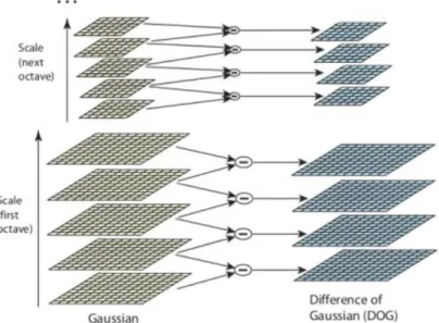
Scale-Invariant Feature Transform (SIFT) is an algorithm in computer vision to detect and describe local features in images, proposed by Lowe (2004). The SIFT descriptor is invariant to consistent scaling, orientation, illumination changes, and partially in-variant to affine transformation. There are four main steps in SIFT algorithm. The first step is scale-space extrema detection. As known, it is impossible to use the same window to detect keypoints with different scale. Therefore, SIFT makes use of DoG, which is obtained as the difference of Gaussian blurring of an image with two dif-ferent values. It is processed for various octaves of the image in Gaussian Pyramid, shown in 2.2. After obtaining DoG, the images can be found for local extrema through scale space. After getting the potential locations for keypoints, SIFT is required to acquire more precise results as refinement because scale-space extrema detection gen-erates few unstable keypoints. The aim of this step is to remove the low contrast keypoints. Besides, the DoG is sensitive to edges so that it is necessary to be removed according to the detector of Harris corner. After that, orientation is assigned to each keypoint to keep invariance to image rotation. A neighborhood is taken around the keypoint location depending on the scale, and the gradient magnitude and direction is calculated in that region for all pixels around the keypoint using equation 2.3. The most important gradient orientations are identified using the histogram. Lastly, the
keypoint descriptor is generated, and a 16*16 neighborhood around the keypoint is taken. It is divided into 16 sub-blocks of 4*4 size. For each sub-block, 8 bin orienta-tion histogram is created. Therefore, a total of 128 bin values are generated. SIFT descriptor representation is designed to avoid the problems of boundary changes in location, orientation and scale do not cause radical changes in the feature vector.
Figure 2.2: DoG representation (Sinha, 2017)
Figure 2.3: Gradient magnitude and orientation (Sinha, 2017)
Speeded up robust feature (SURF), was proposed by Bay, Tuytelaars, and Van Gool (2006), is local feature descriptor inspired by SIFT descriptors. The SURF descriptor is based on the same principles and steps as SIFT. However, the details are different. The algorithm contains three critical steps, including interest point detection, local neighborhood description, and matching. The SURF was designed to the approxi-mation to LoG with box filter, which is the better to calculate the convolution using box filter for integral images. Besides, the SURF depends on the determination of Hessian matrix for both scale and location. During the step of orientation assignment,
the SURF makes use of wavelet responses in horizontal and vertical direction for a neighborhood, and also, enough Gaussian weights are applied to it. The dominant orientation is estimated by calculating the sum of all responses within a sliding ori-entation window of angle 60 degrees. Then, a square region is extracted in order to describe the region around the points. The point of interest is divided into 4x4 square sub-regions, and the Haar wavelet responses are extracted at 5x5 regularly sample points. Compared to SIFT, the SURF can accelerate the calculation process since it employs 64-dimensional feature vector to describe the local feature as advantages rather than 128 dimensions in SIFT.
Furthermore, the Histogram of Oriented Gradient (HOG) was proposed to extract local features in images, which is the variant of SIFT (Dalal & Triggs, 2005). In this research, it indicated that the HOG provides the excellent performance relative to other existing feature sets including wavelets. Also, Ojala, Pietikainen, and Maenpaa (2002) proposed the approach of Local Binary Patterns (LBP) to extract the spatial information of the texture with the invariant to monotonic transformations of the gray levels. In a nutshell, the different approaches of feature extraction in image processing, global feature and local feature, could deliver the different performance because of the existence of various situations for images, such as scalability, illumination, and rotation. Hence, the performance of each approach should be multiple evaluated by different image datasets for image classification.
2.2
BoVW methodology
2.2.1
Introduction
Initially, the methodology of bag-of-words (BoW) is commonly used in the field of natural language processing and information retrieval, such as text categorization, and the term of BoW was early proposed by Z. S. Harris (1954) in a linguistic context. This model aims to represent texts with the number of times a term appears in the texts without the consideration of grammar and word order. After years, the methodology of BoVW was inspired by BoW model in the field of computer vision, proposed by
Csurka et al. (2004). In the process of image classification, a visual word is used in the BoVW model, generated by clustering low-level visual features of local regions points, such as color and texture along with the process of vector quantization. In other words, the BoVW is a sparse vector of occurrence counts of a vocabulary of local image features, which can be described as a histogram of visual words as well. It is possibly amazing that the BoVW schema could be effective and productive to match or surpass the other state-of-the-art performance in some developed applications because of the lack of spatial information and structure. However, the lack of spatial relationships between patches could lead to the issue of high misclassification rate in computer vision.
2.2.2
BoVW process
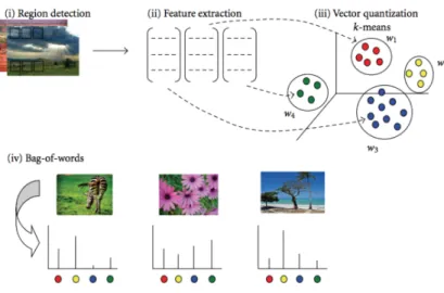
The process of creating BoVW model is shown in figure 2.4, which can be concluded to four key steps as follows. Firstly, it is to detect regions or points of interest. Then, computing local descriptors over those regions or points. After that, quantizing the descriptors into words to form the visual vocabulary. Lastly, finding the occurrences for each specific word in the vocabulary for constructing the BoVW model, namely the histogram of word frequencies (Tsai, 2012).
Figure 2.4: The process of generating BoVW model (Tsai, 2012)
of images. It is computed at predefined locations and scales, and also some popular detection methods were discussed by Mikolajczyk, Leibe, and Schiele (2005). In their research, they compared some well-known detectors based on affine normalization, and the conclusion is that the Hessian-Affine detector outperforms among others. Addi-tionally, the interest points are detected by both sparse and dense approach (Horster & Lienhart, 2007). The interest points are detected at local extrema in the DoG pyramid for sparse features (Lowe, 2004). For dense features, the interest points are defined at sampled grid points.
Computing feature descriptor is an important step to decide how to represent the neighborhood of pixels near the localized region apart from making the decision where features exist in images. In BoVW literature, the SIFT descriptor (Lowe, 2004) is widely used as feature descriptors. In addition, SURF is the alternative to SIFT descriptor, and it has been widely used and applied as well (Bay et al., 2006). The process of SURF contains the procedures of feature detection and description. The purpose of SURF is to produce the similar features as produced by SIFT on Hessian-Laplace interest points, but more effective and accurate. In the study (Mikolajczyk et al., 2005), there has the comparison of some feature descriptors and concludes that the SIFT-based descriptors outperform the other descriptors in many areas. According to the study (Mikolajczyk & Schmid, 2005), the authors compared the performance of local descriptors, which are extracted by the Harris-Affine detector, and it indicated that SIFT-based descriptors deliver the best performance.
After detecting regions and extracting features for images, the final step of con-structing the visual vocabulary for BoVW model is in accordance with vector quan-tization. Basically, the k-means clustering algorithm is used during this step, and the number of visual words generated is based on the number of clusters predefined. van de Sande, Gevers, and Snoek (2011) explained that the process of vector quantiza-tion during building BoVW model has the high computaquantiza-tional cost using the k-means algorithm, which is to find the k number of neighbor clusters for each point. However, there have the limitations of creating the visual vocabulary in the traditional BoVW model, that is, it ignores the spatial information for images because of its orderless
collection. Therefore, Lazebnik, Schmid, and Ponce (2006) proposed the approach of spatial pyramid matching, treated as an alternative consideration of the orderless images. This method can allow the BoVW model to contain the spatial information during the process of generating visual vocabularies to improve the performance of image processing.
2.2.3
Related work
Medical science
Due to the rapid development of modern medical facilities, increasingly numerous medical images are captured and generated. For example, more than 640 million med-ical images have been stored over 100 National Health Service Trusts in UK in 2008 (Khaliq, Blakeley, Maheshwaran, Hashemi, & Redman, 2010). However, there have some special difficulties to classify images on the sizable medical database, such as im-balance number of training images among different classes, intra-class variability, and inter-class similarity. The research presented a BoVW-based approach to obtain high classification accuracy on ImageCLEF 2007 medical database, and the methodolo-gies are based on BoVW for feature extraction with SIFT descriptors and the kernel of radial basis function of support vector machine classifier used in training phrase (Zare, Seng, & Mueen, 2013). Also, magnetic resonance imaging (MRI) is a powerful, non-invasive medical imaging technique widely used in neuroscience and brain disease research (Fatahi, Speck, et al., 2015), and in recent years BoVW has used to analyze MRI to complete the tasks of image classification. Daliri (2012) proposed the BoVW model with the feature extraction of SIFT descriptors from different slides in MR im-ages and used SVM to classify them. Furthermore, Rueda, Arevalo, Cruz, Romero, and Gonz´alez (2012) proposed the model of BoVW model for brain MR images with the features of gray pixel intensities, based on SVM. As can be seen, the BoVW pattern will be further developed to the filed of medical science in the future.
Aerial imagery
The high spatial resolution (HSR) images can be captured and generated by devices, such as satellites and radars, in the domain of aerial imagery. The HSR aerial images can provide abundant spatial and textural information for classification (Xu, Fang, Li, & Wang, 2010). Therefore, the factors of feature detection and description are the crucial points in HSR image classification. Recently years, the BoVW model in image semantic analysis has been considered to improve image processing by many researchers. This state-of-the-art approach of image processing has been successfully applied to general visual categorization (Perronnin, 2008), texture categorization (Qin, Zheng, Jiang, Huang, & Gao, 2008) and object classification of aerial image (Xu et al., 2010). As concerned, the image classification based on BoVW model will be effectively and widely used in the filed of aerial imagery to improve military defense and civil applications.
Robotics
With the development of robotics over decades, the designed robots are purposed to assist human beings to complete tasks. Also, during the awareness process of robots, the image recognition is the necessary progress to allow robotic system to understand what images present. Recently years, the BoVW model has been developed to enhance the process of image classification in robotic system, such as robot navigation and mapping (Nicosevici & Garcia, 2012) and handicapped assistance (Ergene & Durdu, 2017). In the paperwork Nicosevici and Garcia (2012) explained that while discarding the geometric information in images, BoVW proved to be very robust methods to detect visual similarities between images, allowing efficient loop-closure detection even in the presence of illumination and camera perspective changes and partial occlusions. Besides, Ergene and Durdu (2017) proposed to make use of BoVW model to build the visual vocabulary to produce image classification on robotic hands with linear SVM. As the consideration of robotics development, the BoVW could have the potentially great effect on the image recognition in the domain of robotics in the future.
2.3
Image classification
2.3.1
Overview
Image classification is one of the fundamental problems in the domain of computer vision, which has attracted many attentions over the last decade. The goal of image classification is to predict the categories of the input images using its features. The image classification contains four main steps (Kamavisdar, Saluja, & Agrawal, 2013). First of all, the image pre-processing is important preparation before feature extraction to improve the quality of features, such as noise removal, image transformation, and principal component analysis. After that, the feature detection and extraction are conducted to generate the set of descriptors to describe images. Then, the training stage aims to train the selection of the particular features that describes the pattern at best with the machine learning algorithms. Lastly, the testing stage categorizes detected objects into predefined classes by using the suitable method that compares the image patterns with the target patterns.
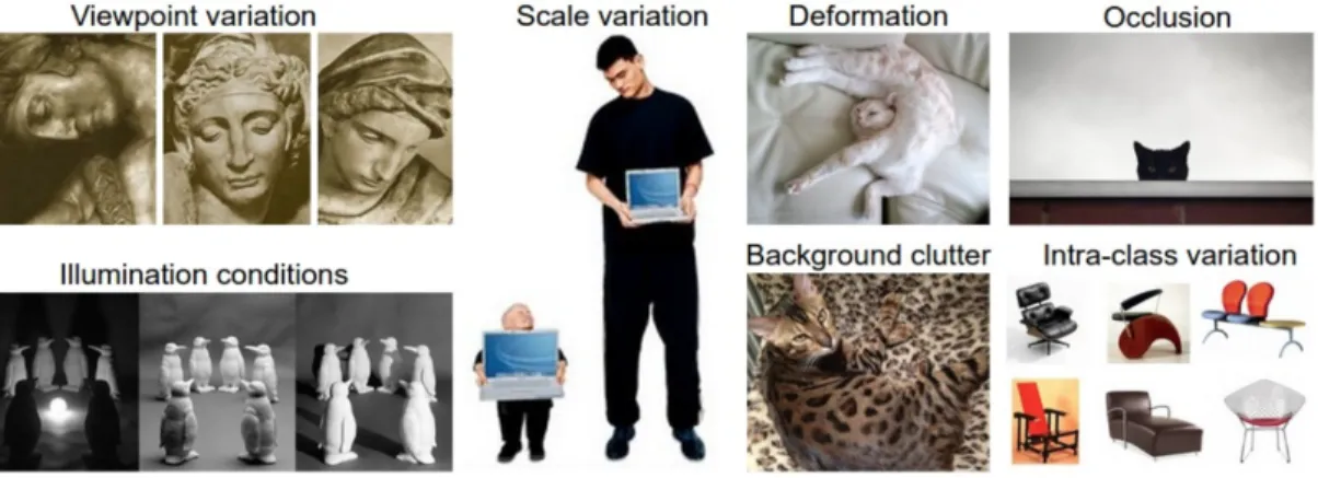
Figure 2.5: The Summary of image classification challenge (Johnson, 2017)
Furthermore, it still has many difficulties and challenges in image classification (Kurian & Karunakaran, 2012). The effect of illumination is sensitive to the pixel level that could cause the significant variations in the intensity of the pixels. A single object can be oriented in many ways concerning the camera by changing position while capturing that lead to the problem of viewpoint variation. Also, the visual objects
often exhibit variation for their sizes in the real world, and the most of objects do not have the rigid feature that can be deformed in extreme ways. Furthermore, the objects of interest could mix into their background, making them difficult to identify. And the objects can be occluded, only the small part of an object can be visible. In addition, the object classes can often be relatively broad. There could have many different types of these objects with the different appearance. The summary of challenges in image classification is shown in figure 2.5.
2.3.2
Machine learning approaches
Generally, there are two types of approaches in machine learning, which are the su-pervised learning for labeled data and unsusu-pervised learning for unlabeled data. Su-pervised learning is to infer a function from labeled training data. It analyzes the training data and produces an inferred function, which can be mapped to the data to be assigned labels. Unsupervised machine learning is to infer a function to describe the hidden structure from unlabeled data, which means the information of categorization is not included in the observations. This approach is not widely used in the task of image classification, but it is used to generate the visual vocabulary in BoVW model, such as using k-means algorithm (Csurka et al., 2004).
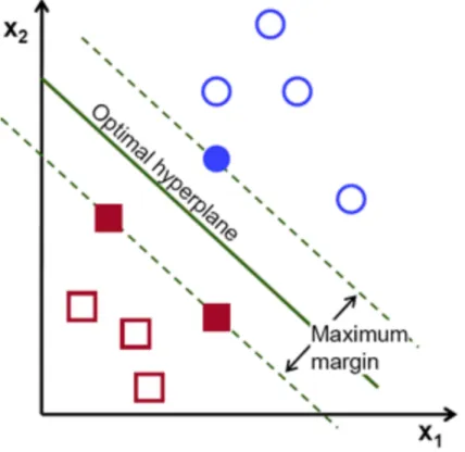
Support Vector Machine (SVM) is the state-of-the-art supervised machine learning technique that is widely used in image classification. SVM builds the set of hyper-planes in a high or infinite dimensional space, which can be used for classification, regression, and outliers detection. The hyperplanes in SVM can be adjusted within the maximum margin, shown in figure 2.6. In many situations, it indicated that classi-fication results in the issue of over-fitting in high dimensional feature spaces, however, in SVM over-fitting is controlled through the principle of structural risk minimization (Cortes & Vapnik, 1995). The problem of misclassification is minimized by maximizing the margin between the points and the boundary (Mashao, 2003).
Figure 2.6: SVM representation
The SVM is naturally used for binary classification. However, it also can be ex-tended to multi-class image classification, along with the strategies of one-against-one and one-against-all (Melgani & Bruzzone, 2004). The one-against-all inspires the most common SVM multi-class approach and involves the division of an N class dataset into N two-class cases. Also, the one-against-one approach consists in building a machine for each pair of classes resulting in N(N-1)/2 machines. Each classification gives one vote to the winning class, and the point is labeled with the class having most votes while applied to a test point. This approach can be further modified to weight in the voting process. In the research (Gualtieri & Cromp, 1999), it explained that the one-against-one approach outperforms one-against-all, because one-against-all can be compromised according to unbalanced training datasets. Additionally, the kernel method, called kernel trick as well, also plays a significant role in SVM-based classifi-cation. In fact, the state of linear is extraordinary, and the systems in the real world are not truly linear. Therefore, the non-linear model is suitable to solve the problem
of non-linearity rather than the linear model. There have some non-linear kernel func-tions with SVM, including polynomials and Radial Based Function. In a word, SVM gains flexibility in the choice of the form of the threshold and contains a nonlinear transformation. It also provides an excellent generalization capability, resulting in the reduction in computational complexity and simplicity of making decision rules.
Random Forest is another very successful classification algorithm, which was pro-posed as a combination of tree predictors so that each tree depends on the values of a random vector sampled independently with the same distribution for all trees in the forest (Breiman, 2001). In another word, it is a pattern for constructing a clas-sification ensemble with the set of decision trees, growing in the randomly selected subspace of data. It can be applied to object classification with the relatively small number of classes (Moosmann, Triggs, & Jurie, 2007). Also, the attractions of ran-dom forests have been widely developed in image classification (Bosch, Zisserman, & Munoz, 2007). Some approaches have been proposed to build random forest models from subspaces of data (Breiman, 2001; Ho, 1998). One of the most well-known forest structure, proposed by Breiman (2001), is to randomly select a subspace of features at each node to grow branches of decision trees, then to use bagging method to generate training data subsets for building individual trees, finally to combine all individual trees to form random forests model. In addition, owing to the image features of high dimensionality sparsity and multi-class labels, they could contain the uninformative feature, resulting in the problem of serious misclassification. Within the process of constructing forest, informative features could be possibly missed with the selection of small subspace from high dimensional data (Amaratunga, Cabrera, & Lee, 2008). In a nutshell, the over-fitting, mentioned before, is a serious problem, resulting in the unexpected data. However, the classifier does not tend to over-fit the model when enough trees are involved in the forest for the random forest algorithm. Then, the other advantage for random forest is that it can deal with missing values. Moreover, it is difficult to conclude that there was a significant difference performance between ran-dom forest and SVM used in image classification, and the different data distribution and various unexpected factors could significantly impact on image classification.
2.3.3
Evaluation measurement
The evaluation is the most significant stage after obtaining the classification results. Therefore, it can report how the performance of classifiers and even the performance of feature extraction approaches in image classification. With the respect of classifica-tion accuracy, it is commonly described as a metric computed from confusion matrix (Provost, Fawcett, Kohavi, et al., 1998) according to the testing sets, and also, it is es-timated by different classifications, compared to indicate the significance of differences in the classification results (Foody & Mathur, 2004).
Typically, the confusion matrix contains the information about actual and pre-dicted classifications done by the classification pattern. The following table 2.1 de-scribes the confusion matrix for a two-class classifier where the term of true positives (TP) is the number of correct predictions that an instance is positive, the term of false positive (FP) is the number of incorrect predictions that an instance is positive, the term of false negatives (FN) is the number of incorrect of predictions that an instance negative, and term of true negatives (TN) is the number of correct predictions that an instance is negative.
Predicted Positive Predicted Negative Actual Positive True Positives (TP) False Negatives (FN)
Actual Negative False Positives (FP) True Negatives (TN) Table 2.1: Confusion Matrix
According to the representation of confusion matrix, the common and intuitive measure is calculated as the number of all correct predictions divided by the total number of the datasets, known as accuracy that is shown in equation 2.1.
Accuracy= T P +T N
T P +F P +T N +F N (2.1)
Furthermore, the other measurement still plays a crucial role in the evaluation of classification that are sensitivity and specificity. Sensitivity, also called recall or true
positive rate, is calculated as the number of correct positive predictions divided by the total number of positives, shown in equation 2.2.
Sensitivity = T P
T P +F N (2.2)
Specificity, also called true negative rate, is calculated as the number of correct negative predictions divided by the total number of negatives, shown in equation 2.3.
Specif icity = T N
T N +F P (2.3)
Additionally, precision, called positive predictive value, is calculated as the number of correct positive predictions divided by the total number of positive predictions, shown in equation 2.4.
P recision= T P
T P +F P (2.4)
2.4
Statistical test
Over the last decade, the field of machine learning has been increasingly aware of the need for statistical validation of comparisons (Demˇsar, 2006). Dietterich (1998) examines McNemars test on misclassification matrix as powerful as the 52 cv t-test in the case of the unreliability of running the algorithm morn than once, and using t-test is discouraged after cross validation. Nadeau and Bengio (2000) proposed the corrected re-sampled t-test that adjusts the variance over subsets of examples. However, none of the studies above found the approach to cope with evaluating the performance of multiple classifiers and the performance of classifiers, tested by multiple datasets. Therefore, the non-parametric testing is proposed to compare classifiers in information retrieval (Sch¨utze, Hull, & Pedersen, 1995). And also, V´azquez, Escolano, Ria˜no, and Junquera (2001) studied ANOVA (Fisher, 1956) and Friedman’s test (Friedman, 1940) for comparison of multiple models on single data.
As discussed above, the Friedman test is a non-parametric equivalent of the repeated-measures ANOVA, along with the ranks of the algorithms for each dataset. The
statistic of Friedman is distributed based on χ2F with k-1 degrees of freedom, shown in equation 2.5. (Demˇsar, 2006). It can identify whether the significant difference appears over multiple datasets.
χ2F = 12N k(k+ 1) X j Rj2−(k(k+ 1) 2) 4 (2.5)
The Nemenyi test (Nemenyi, 1962), treated as post-hoc test, is used to compare all classifiers to each one when null-hypothesis is rejected in Friedman test. It indicates which paired classifiers have the significant difference over multiple datasets if the corresponding average ranks differ by at least the critical difference, shown in equation 2.6.
CD =qα r
k(k+ 1)
6N (2.6)
Additionally, the table 2.2 describes the critical values for the two-tailed Nemenyi test, as using after Friedman test.
#approaches 2 3 4 5 6 7 8 9 10
q0.05 1.960 2.343 2.569 2.728 2.850 2.949 3.031 3.102 3.164
q0.10 1.645 2.052 2.291 2.459 2.589 2.693 2.780 2.855 2.920
Table 2.2: Critical values for the two-tailed Nemenyi test (Demˇsar, 2006)
2.5
Conclusion
This chapter reviewed regarding peer-reviewed papers in details, along with the field of image classification based on BoVW model in computer vision. First of all, in the sec-tion 2.1, the prior procedure of image classificasec-tion, known as image processing, were studied, including both representations of global feature and local feature. Further-more, the stages of feature detection and feature description while representing local feature were extensively discussed, and also, the state-of-the-art feature descriptors were introduced and compared, such as SIFT, SURF, and HOG. Next to the section 2.2, it reviewed the model of BoVW used in the task of image classification, along
with the relevant research work in different domains. Then, the process of generating BoVW was introduced and discussed in details. Also, the different selections of the approaches during the process of generating BoVW model were extensively discussed and compared, such as the selections of feature descriptors and the selections of vector quantization algorithms. In addition, the limitations of BoVW model were presented and explained as well.
After that, in the section 2.3 the overview of image classification were introduced at the high level, including the general process and its challenges. The supervised machine learning algorithms were considered to introduce in general, and the SVM and random forest were intensively discussed and compared in image classification. Additionally, the measurement of classification evaluation was presented and described with a little math knowledge. Furthermore, the section 2.4 was intensively discussed, and also the Friedman test and the relevant post-hoc test was deeply introduced and studied with a little math knowledge.
The next chapter, namely experiment design and methodology, will be presented to design the methodologies and experimental software for image classification based on the proposed research question in chapter 1 and the existing literature reviews in this chapter.
Experiment design and
methodology
3.1
Introduction
In this chapter, the experiments are designed and presented in details for this research, including the descriptions of image datasets, the methodologies of all experiments, the design of experimental software, and the conclusion of this chapter. The structure of this chapter is described as following. Firstly, in the section of data used, the image data sources will be described in general and illustrate its advantages. Secondly, in the section of evaluation methodology, the methodology will be presented in the aspects of approaches, performance measures, statistical tests. Thirdly, in the section of experimental software design, the detailed software structure will be designed and presented. Finally, the conclusion of this chapter will be presented, and describe what it will go through in the next chapter.
3.2
Data used
As the part of this research, the data source selection plays a significant role in the process of image classification, since it can impact on classification performance. The image data source, called Caltech-256, is used to the task of image classification for this
research. The original version, called Caltech-101 (Fei-Fei, Fergus, & Perona, 2007), was collected by selecting a set of object categories that downloaded instances from Google Images, and then manually screening out all images that did not fit the cate-gory. However, Caltech-256 was collected in similar methods with some improvements, such as more than a double number of categories, the increase of minimum number of images for any category from 31 to 80, and the avoiding of artifacts because of image rotation (Griffin et al., 2007). The summary between Caltech-101 and Caltech-256 is illustrated in table 3.1. As can be seen, there has a dramatic improvement from Caltech-101 to Caltech-256, including the number of categories, total images and min-imal instances for each category. Therefore, the Caltech-256 is conducted to involved in image classification experiments to answer research question defined in the previous chapter.
Dataset Released Categories Images total Min Med Mean Max
Caltech-101 2003 101 9144 31 59 90 800
Caltech-256 2006 256 30607 80 100 119 827
Table 3.1: Comparison between Caltech101 and Caltech256. The clutter categories are excluded.(Griffin et al., 2007)
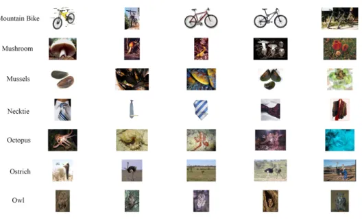
The datasets will be determined to select from Caltech-256 and use to both exper-iments of binary classification and multi-class classification, which will be discussed and presented in details in the next chapter. Classification across all 256 images is a complex process so separate binary and multi-class datasets were extracted from the source data. It is time-consuming and dependent on the high-quality personal computer or laptop. Therefore, the dataset used to binary classification experiment contains 21 paired-category sub-datasets, assembled from 7 categories that are moun-tain bike, mushroom, mussels, necktie, octopus, ostrich and owl from Caltech-256, shown in table 3.2 and figure 3.1. Besides, BD(i) denotes that the ith sub-dataset for binary classification experiment. In a word, each sub-dataset only contains two categories with the same number of instances for each category. For example, The cat-egories of mountain bike and mushroom both have 82 instances in BD1 sub-dataset.
Classes #Instances BD1 mountain bike, mushroom 82, 82 BD2 mountain bike, mussels 82, 82 BD3 mountain bike, necktie 82, 82 BD4 mountain bike, octopus 82, 82 BD5 mountain bike, ostrich 82, 82 BD6 mountain bike, owl 82, 82 BD7 mushroom, mussels 174, 174 BD8 mushroom, necktie 103, 103 BD9 mushroom, octopus 111, 111 BD10 mushroom, ostrich 109, 109 BD11 mushroom, owl 70, 70 BD12 mussels, necktie 103, 103 BD13 mussels, octopus 111, 111 BD14 mussels, ostrich 109, 109 BD15 mussels, owl 70, 70 BD16 necktie, octopus 111, 111 BD17 necktie, ostrich 103, 103 BD18 necktie, owl 70, 70 BD19 octopus, ostrich 111, 111 BD20 octopus, owl 70, 70 BD21 ostrich, owl 70, 70
Table 3.2: The summary of datasets for binary classification
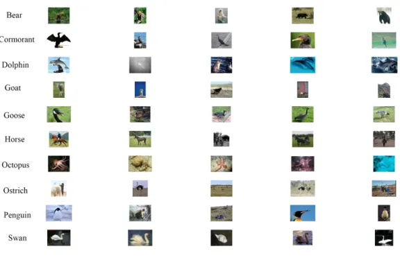
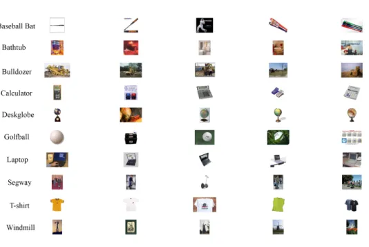
The generated dataset for multi-class classification experiment is shown in table 3.4 and figure 3.2 for Group A, and table 3.5 and figure 3.3 for Group B. The MDA(i) and MDB(i) denotes that the ith dataset in Group A and the ith dataset in Group B for multi-class classification experiment, respectively. Each category is related to the class of animal in group A, and each category is randomly selected from the rest of categories, which do not belong to the class of animal in group B. Therefore, there has a difference that group A contains similar categories and images, and group B contains non-relevant categories and images. Each group contains eight sub-datasets that the number of classes is increasing from 3 classes to 10 classes. And also, the latter sub-dataset is generated by adding a new category, based on the former. For example, MDB1 has the categories that are baseball bat, bathtub and bulldozer, and MDB2 has the categories that are baseball bat, bathtub, bulldozer, and calculator. In addition, each sub-dataset contains the same number of instances for each category, based on the minimal number of instances among categories. It can keep balance for the proportion of each category in one sub-dataset to deliver the correct classification results.
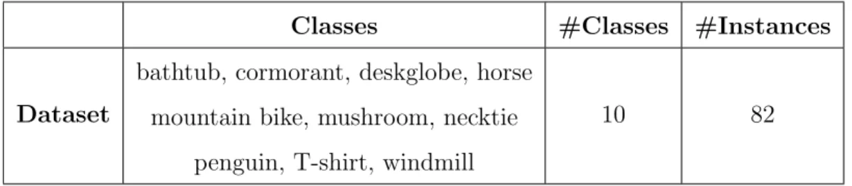
In addition, the dataset, designed for the experiment of selecting vocabulary size , is displayed in table 3.3. It contains ten classes, which are randomly selected and obtained from both used datasets of binary classification experiment and multi-class classification experiment. As can be seen, the types of categories, such as animal-relevant and non-animal-relevant, would not impact on the results in the process of vocabulary size selection. In another word, the results of this experiment are yielded, excluding the influence of samples selection.
Classes #Classes #Instances
Dataset
bathtub, cormorant, deskglobe, horse mountain bike, mushroom, necktie
penguin, T-shirt, windmill
10 82
Classes #Classes #Instances
MDA1 bear, cormorant, dolphin 3 102
MDA2 bear, cormorant dolphin, goat
4 102
MDA3 bear, cormorant, dolphin goat, goose
5 102
MDA4 bear, cormorant, dolphin goat, goose, horse
6 102
MDA5
bear, cormorant, dolphin goat, goose horse,octopus
7 102
MDA6
bear, cormorant, dolphin goat, goose, horse
octopus, ostrich
8 102
MDA7
bear, cormorant, dolphin goat, goose, horse octopus, ostrich, penguin
9 102
MDA8
bear, cormorant, dolphin, goat goose, horse, octopus ostrich, penguin, swan
10 102
Table 3.4: Multi-class Classification: Group A (Animal-relevant Class)
Classes #Classes #Instances MDB1 baseballbat, bathtub, bulldozer 3 82 MDB2 baseballbat, bathtub bulldozer, calculator 4 82 MDB3 baseballbat,bathtub,bulldozer calculator,deskglobe 5 82 MDB4 baseballbat,bathtub,bulldozer calculator,deskglobe,golfball 6 82 MDB5 baseballbat,bathtub,bulldozer calculator, deskglobe golfball, laptop 7 82 MDB6 baseballbat,bathtub,bulldozer calculator,deskglobe,golfball laptop,segway 8 82 MDB7 baseballbat,bathtub,bulldozer calculator,deskglobe,golfball laptop,segway,T-shirt 9 82 MDB8 baseballbat,bathtub,bulldozer calculator,deskglobe,golfball,laptop segway,T-shirt,windmill 10 82
Table 3.5: Multi-class Classification: Group B (Non-relevance Class)
3.3
Evaluation methodology
In this section, the general evaluation methodologies are stated and described in the aspects of approaches, performance measures and statistical test, and these method-ologies will be applied to all experiments.
3.3.1
Approach
As the discussion made about the purpose of this research and the description of datasets, the selected datasets will be divided into 2 partitions, treated as the training sets and the testing sets to implement the process of image classification. In the meantime, the proportion of partitions are set as 70% for training sets and 30 % for testing sets.
Figure 3.4: The flow chart of the supervised image classification
The flow chart 3.4 is designed to illustrate the fundamental stages during the process of image classification. In general, it contains training stage and testing stage. In the training stage, the images are conducted to the process of feature extraction, such as global feature and BoVW model along with the local feature. Then, the extracted features are trained with SVM algorithm to generate the SVM classifier model. According to the paperwork (Csurka et al., 2004), it empirically proved that the SVM classifier delivers the best performance for the task of image classification over the other supervised machine learning classifiers. In the testing stage, the images to be tested are processed using the same approach of feature extraction, and the
classification results are generated by the corresponding classifier model. Moreover, the linear SVM with one-against-one approach will be used in the experiment of multi-class multi-classification.
Additionally, the number of iterations for all experiments runs is set as three times so that it can provide the robustly experimental results. Besides, the results generated by this way can be conducted to statistical test to prove the correctness of hypotheses given by Chapter 1. Also, some approaches of image processing, introduced and dis-cussed in chapter 2, will be used to present images before entering the training stage, such as raw pixels and color histogram representation, and BoVW pattern with the SIFT and SURF descriptors, respectively. Furthermore, the different designed exper-iments, given by Chapter 4 in details, will make use of the approaches as mentioned earlier approaches to present images based on the purpose of each experiment.
3.3.2
Performance measures
The most important part of this research is to evaluate the given results by the con-ducted experiments so that it can achieve and conclude the aim of this research. In the field of image classification, the confusion matrix is the popular and proper method to evaluate the performance of classifiers, even the performance of image processing methods. In another word, the confusion matrix is usually used as the quantitative method of characterizing image classification accuracy. For all designed experiments in this research, the average accuracy will be calculated based on the output of con-fusion matrix, and it also will be used in the stage of statistical test in order to find whether the significant difference exists during groups.
3.3.3
Statistical test
The statistical test provides a mechanism for making quantitative decisions about processes, and also statistical methodologies are required to make sure that the data is interpreted correctly and that apparent relationship is significant and not merely chance occurrences. Therefore, it is the essential procedure after obtaining the results,
given by experiments in this research. In addition, the average accuracy, obtained by confusion matrix, is not sufficient to prove the defined hypotheses, since it could lead to the problem of different conclusions due to the samples selection during experimen-tations.
As the designed datasets for experiments, there have some comparisons between the different approaches of image processing over multiple datasets. Therefore, the non-parametric test, called Friedman test, will be applied to find out the differences between each image processing approach without the assumption of normal distribu-tion test (Demˇsar, 2006). However, the Friedman test only can reveal whether there have the differences over multiple datasets, but it cannot indicate whether the sig-nificant differences exist for each approach of image process again the other one. To solve this problem, the post-hoc test is proposed to process if the null-hypothesis is re-jected. The Nemenyi test is used when all image processing approaches are compared to each other (Demˇsar, 2006) in order to explain the significant difference between the performance of two approaches based on the corresponding average ranks differ by at least the critical difference. The formula for calculating critical value is displayed in equation 2.6, and the table of critical value is shown in table 2.2.
3.4
Experimental software design
3.4.1
Development environment
All experiments will be carried out using a MacBook pro with the macOS High Sierra that is version 10.13.2, and the hardware is displayed in table 3.6. Besides, the designed software will be implemented in MATLAB with the version of R2017b 64bit under academic license.
Furthermore, the computer vision toolbox, supported by MATLAB, provides a comprehensive suite of algorithms and tools for object detection and recognition. The system toolbox is a suite of several machine learning, feature-based, and motion-based techniques for object detection and recognition. Also, the VLFeat open source library with the version of 0.9.20, treated as third-party package in this research, implements
Type of Hardware Description Processor Name Intel Core i7
Processor Speed 2.2 GHZ
Total Number of Cores 4
L2 Cache (per Core) 256 KB
L3 Cache 6 MB
Graphics Intel Iris Pro 1536 MB
Memory 16 GB 1600 MHz DDR3 Table 3.6: Hardware for Development Environment
popular computer vision algorithms specializing in image understanding and local features extraction and matching. It is written in C for efficiency and compatibility, with interfaces in MATLAB for ease of use, and detailed documentation throughout. It supports Windows, Mac OS X, and Linux.
3.4.2
Software design
According to the designed process of image classification above, the relevant coding using MATLAB is designed as follows. The figure 3.5, similar to class diagram, illus-trates the structure of software that will conduct all designed experiments in MAT-LAB. In general, the top level script is main.m for this study, which is proposed to call all functions defined by myself. The functions of extracting features are defined, such as raw pixels extraction, color histogram extraction, SIFT extraction, and SURF extraction. Then, the outputs returned by the function of SIFT extraction and the function of SURF extraction is processed by the function of building the visual vo-cabularies. Besides, the function of SVM classifier is also designed to provide the high-performance classification. This figure indicates what the variables of input and output are presented.
Figure 3.5: The similar class diagram for software design based on MATLAB
3.5
Conclusion
The objective of this chapter is to provide the design of the experiments and method-ologies in order to accomplish the objective of this research, discussed in chapter 1. This chapter begins with the explanations of selecting image data source reasons, and the general methodologies of creating the relevant datasets for all designed experiments as well. Then, the evaluation methodologies are designed and discussed, including used approaches, performance measures, and statistical test. Lastly, the experimental soft-ware is designed and presented that will be applied to all proposed experiments. The next chapter will present the descriptions, results, and evaluations of each experiment in details, and also, the key findings and analysis will be discussed.
Experimentation and results
4.1
Introduction
This chapter presents the details and results of all experiments based on the designed methodologies in Chapter 3. In total, there were three experiments conducted. Firstly, the binary classification experiment is to determine whether BoVW is the best ap-proach of image processing over baseline apap-proaches. Secondly, the aim of multi-class classification experiment is to find out how the performance of BoVW model extends to multiple classes. Lastly, the experiment of selecting vocabulary size presents the importance of vocabulary size selection during the process of creating BoVW on clas-sification results. Furthermore, the evaluation and discussion of results and findings will be presented for all experiments.
4.2
Binary classification experiment
4.2.1
Implementation
Considering the overview of approaches of image processing in the field of image clas-sification in chapter 2, the aim of binary clasclas-sification experiment is to determine which image processing approach can deliver the best performance in the process of image classification using a linear SVM classifier among raw pixels, color histogram,
and BoVW model with SIFT and SURF descriptors, respectively. For performance comparison, on the one hand, the approaches of raw pixels and color histogram are treated as baseline approach, and on the other hand, the BoVW model is treated as state-of-the-art approach with SIFT and SURF descriptors as well, respectively.
The designed dataset to be used in this experiment is illustrated in Table 3.2 in chapter 3. In general, this dataset contains 21 sub-datasets, having only two classes with the same number of instances for each sub-dataset. It is convenient to evaluate the results, generated by this experiment, without the consideration of sample distri-butions. In addition, due to the selection of different parameters, the paper (Lowe, 2004) provides empirical evidence, such as the number of octaves is 4 and number of scale levels is 5. Therefore, the SIFT parameter in this experiment will be set in the same way. And, the images are shrunk to small square resolution with 16 * 16 blocks for the parameter of raw pixel features. Furthermore, as consideration about the influ-ence of vocabulary size during the process of vector quantization for creating BoVW model (Hou, Kang, & Qi, 2010), the vocabulary size is statically defined to 500 that allows to reduction of the computation cost and time with a still high performance of classification. In the linear SVM algorithm is involved in training stage to generate the predictive models for all selected approaches of image processing.
4.2.2
Results and statistical test
As discussed in the literature review, in the binary classification, the accuracy, calcu-lated by the confusion matrix from SVM classifier, is the most common measurement to evaluate the performance of classification on the various approaches of image rep-resentation. Owing to the three iterations during running, the average accuracy is calculated for each sub-dataset in binary classification experiment, where the sum of accuracies and divided by 3. The results of average accuracy for binary classification experiment is shown in table 4.1. Also, for easy viewing results, the multiple his-tograms are provided in figure 4.1, showing the comparison of average accuracy using the different features for each sub-dataset. Besides, the descriptive statistic is provided as well in table 4.2.
As can be seen, the mean accuracy for SURF, regarded as the common measure, is the highest among all feature extraction approaches, which is 0.916, in contrast, the mean of raw pixel is the lowest, which is 0.657. According to the values of range, standard deviation and its error, it indicates that the SURF has the most accurate and stable performance with the less error on feature extraction in image classification. However, it has not been enough to make conclusion so far, because there has a slight difference in the values of mean accuracy between the approaches of SIFT and SURF. It cannot prove which can yield the best performance in the real world without the inferential test. Furthermore, the difference will be statistically tested among all approaches afterward.
RawPixel Color SIFT SURF
BD1 0.78 0.81 0.91 0.92 BD2 0.64 0.74 0.89 0.91 BD3 0.66 0.72 0.91 0.90 BD4 0.72 0.80 0.89 0.88 BD5 0.75 0.81 0.90 0.94 BD6 0.68 0.8 0.92 0.88 BD7 0.66 0.68 0.80 0.85 BD8 0.71 0.82 0.9 0.93 BD9 0.51 0.73 0.89 0.91 BD10 0.73 0.74 0.93 0.94 BD11 0.50 0.68 0.90 0.89 BD12 0.58 0.71 0.87 0.90 BD13 0.64 0.74 0.85 0.91 BD14 0.61 0.73 0.79 0.89 BD15 0.63 0.68 0.95 0.89 BD16 0.70 0.81 0.94 0.93 BD17 0.77 0.82 0.91 0.98 BD18 0.69 0.89 0.95 0.96 BD19 0.70 0.80 0.95 0.94 BD20 0.45 0.76 0.94 0.93 BD21 0.68 0.74 0.96 0.95