Initializing neural networks for hierarchical multi-label text classification

Initializing neural networks for hierarchical multi-label text classification

1_{Computer Laboratory, 15 JJ Thomson Avenue} 2_{Language Technology Lab, DTAL}

University of Cambridge, UK

[email protected], [email protected]

Abstract

Many tasks in the biomedical domain re-quire the assignment of one or more pre-defined labels to input text, where the la-bels are a part of a hierarchical structure (such as a taxonomy). The conventional approach is to use a one-vs.-rest (OVR) classification setup, where a binary clas-sifier is trained for each label in the tax-onomy or ontology where all instances not belonging to the class are considered nega-tive examples. The main drawbacks to this approach are that dependencies between classes are not leveraged in the training and classification process, and the addi-tional computaaddi-tional cost of training par-allel classifiers. In this paper, we apply a new method for hierarchical multi-label text classification that initializes a neural network model final hidden layer such that it leverages label co-occurrence relations such as hypernymy. This approach ele-gantly lends itself to hierarchical classifi-cation. We evaluated this approach using two hierarchical multi-label text classifica-tion tasks in the biomedical domain using both sentence- and document-level classi-fication. Our evaluation shows promising results for this approach.

1 Introduction

Many tasks in biomedical natural language pro-cessing require the assignment of one or more la-bels to input text, where there exists some struc-ture (such as a taxonomy or ontology) between the labels: for example, the assignment of Medical Subject Headings (MeSH) to PubMed abstracts (Lipscomb,2000).

A typical approach to classifying multi-label

documents is to construct a binary classifier for each label in the taxonomy or ontology where all documents not belonging to the class are consid-ered negative examples, i.e. one-vs.-rest (OVR) classification (Hong and Cho, 2008). This ap-proach has two major drawbacks: first, it makes the hard assumption that the classes are indepen-dent which often does not reflect reality; second, it is more computationally expensive (albeit by a constant factor): if there are a very large number of classes, the approach becomes computationally unrealistic.

In this paper, we investigate a simple and com-putationally fast approach for multi-label classifi-cation with a focus on labels that share a structure, such as a hierarchy (taxonomy). This approach can work with established neural network archi-tectures such as a convolutional neural network (CNN) by simply initializing the final output layer to leverage the co-occurrences between the labels in the training data.

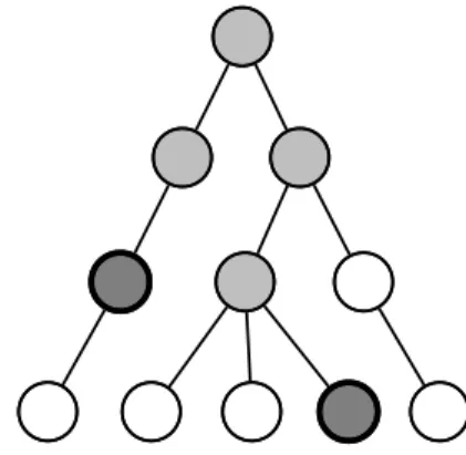
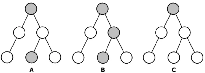
Figure 1: Hierarchical multi-label classification. Nodes represent possible labels that can be as-signed to text: a dark grey node denotes an explicit label assignment and light grey denotes implicit assignment due to a hypernymy relationship with the explicitly assigned label.

First, we need to define hierarchical multi-label classification. In multi-label text classification, in-put text can be associated with multiple labels (la-bel co-occurrence). When the la(la-bels form a hi-erarchy, they share a hypernym–hyponym relation (Figure1). When multiple labels are assigned to the text, if it is explicitly labeled by a subclass it must also implicitly include all of the its super-classes.

The co-occurrence between subclasses and su-perclasses as labels for the input text contains in-formation we would like to leverage to improve multi-label classification using a neural network.

In this paper we experiment with this approach using two hierarchical multi-label text classifica-tion tasks in the biomedical domain, using both document- and sentence-level classification.

We first briefly summarize related literature on the topic of multi-label classification using neural networks, we then describe our methodology and evaluation procedure, and then we present and dis-cuss our results.

2 Related work

There have been numerous works that focus on solving hierarchical text classification. Sun and Lim (2001) proposed top-down level-based SVM classification. More recently, Sokolov and Ben-Hur (2010); Sokolov et al. (2013) predict ontol-ogy terms by explicitly modeling the structure hi-erarchy using kernel methods for structured output space.Clark and Radivojac(2013) use a Bayesian network, structured according to the underlying ontology to model the prior probability.

Within the context of neural networks, Kurata et al.(2016) propose a scheme for initializing neu-ral networks hidden output layers by taking into account multi-label co-occurrence. Their method treats some of the neurons in the final hidden layer as dedicated neurons for each pattern of label co-occurrence. These dedicated neurons are initial-ized to connect to the corresponding co-occurring labels with stronger weights than to others. They evaluated their approach on theRCV1-v2 dataset (Lewis et al.,2004) from the general domain, con-taining only flat labels. Their evaluation shows promising results. However, their applicability to the biomedical domain with more a complex set of labels that share a hierarchy remains an open question.

Chen et al. (2017) propose a convolutional

neural network (CNN) and recurrent neural net-work (RNN) ensemble method that is capable of efficiently representing text features and mod-eling high-order label correlation (including co-occurrence). However, they show that their method is susceptible to overfitting with small datasets.

Cerri et al.(2014) propose a method for hierar-chical multi-label text classification that incremen-tally trains a multi-layer perceptron for each level of the classification hierarchy. Predictions made by a neural network in a given level are used as in-puts to the neural network responsible for the pre-diction in the next level. Their method was eval-uated against several datasets with convincing re-sults.

There are also several relevant works that pro-pose the inclusion of multi-label co-occurrence into loss functions such as pairwise ranking loss (Zhang and Zhou,2006) and more recent work by

Nam et al. (2014), who report that binary cross-entropy can outperform the pairwise ranking loss by leveraging rectified linear units (ReLUs) for nonlinearity.

3 Method

In this section, we describe the approach of initial-izing a neural network for multi-label classifica-tion. We base ourCNNarchitecture on the model ofKim(2014), which has been used widely in text classification tasks, but this approach can be ap-plied to any other architecture.

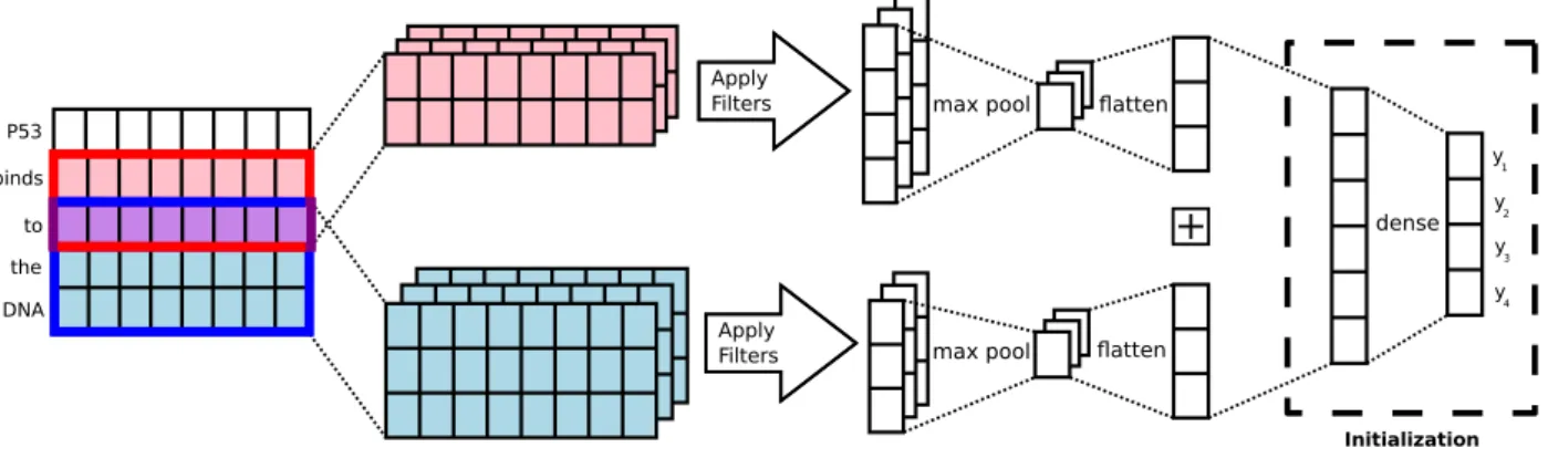
Briefly, this model consists of an initial embed-ding layer that maps input texts into matrices, fol-lowed by convolutions of different filter sizes and 1-max pooling, and finally a fully connected layer. The architecture is illustrated in Figure2.

To perform multi-label classification using this architecture, the final output layer uses logistic (sigmoid) activation functionσ:

σ(x) = 1

1 + e−x (1)

wherexis the input signal. The output range of the function is between zero and one; if it is above a cut-off thresholdTσ(which is tuned by grid search on the development dataset) then the predictiony0

k for label yk is positive. We use a binary cross-entropy loss functionL:

L(θ,(x, y)) =−XK k=1

yklog(yk0)+(1−yk) log(1−y0k) (2) where θ is the model parameters andK is the number of classes.

As shown in Figure 2, the multi-label initial-ization happens in output layer of the network. Figure3illustrates the initialization process. The rows represent the units in the final hidden layer, while the columns represent the output classes.

The idea is to initialize the final hidden layer with rows that map to co-occurrence of labels in the training data. This can be implicit hy-pernymy relations between the labels, or explicit occurrence in the annotation. For each co-occurrence, the valueω is assigned to the associ-ated classes and a value of zero is assigned to the rest. The valueωis the upper bound of the normal-ized initialization proposed byGlorot and Bengio

(2010), which is calculated as follows:

ω =

√

6

√

nh+nk (3)

wherenhis the number of units in the final hidden layer andnk is the number of units in the output layer (i.e. classes). This value was also success-fully used byKurata et al.(2016) in their initial-ization procedure.

The motivation for this initialization is to incline units in the hidden layer to be dedicated to repre-senting co-occurrence of labels by triggering only the corresponding label nodes in the output layer when they are active.

The number of units in the final hidden layer can exceed the number of label co-occurrences in the training data. We must therefore decide what to do with the remaining hidden units. Kurata et al.

(2016) assign random values to these units (shown in Figure3(B)). We will also use this scheme, but in addition we propose another variant: we assign the value zero for these neurons, so that the hid-den layer will only be initialized with nodes that represent label co-occurrence.

We implement the neural network and the ini-tialization using Keras (Chollet,2015). the hyper-parameters for our model and baselines are those ofKim(2014), summarized in Table1.

We use word2vec embeddings trained on PubMed byChiu et al.(2016).

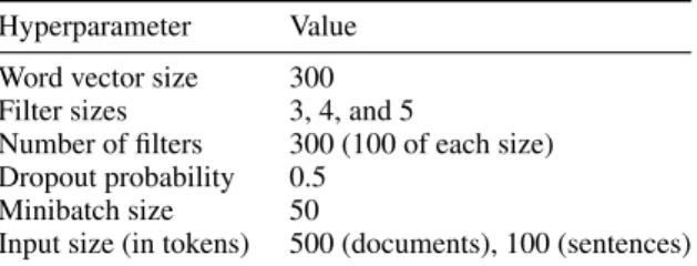
Hyperparameter Value Word vector size 300 Filter sizes 3, 4, and 5

Number of filters 300 (100 of each size) Dropout probability 0.5

Minibatch size 50

Input size (in tokens) 500 (documents), 100 (sentences) Table 1: Our baseline model, based onKim(2014) model hyperparameters.

4 Data

We investigate our approach using two multi-label classification tasks. In this section, we describe the nature of these tasks and the annotated gold standard data.

Task 1: The Hallmarks of Cancer The

Hall-marks of Cancer describe a set of interrelated bi-ological properties and behaviors that enable can-cer to thrive in the body. Introduced in the sem-inal paper by Hanahan and Weinberg (2000)— the most cited paper in the journalCell—the hall-marks of cancer have seen widespread use in BioNLP for many systems and works, including the BioNLP Shared Task 2013, ‘Cancer Genetics task’ (Pyysalo et al.,2013), which involved the ex-traction of events (i.e. biological processes) from cancer-domain texts. Baker et al.(2016) have re-leased an expert-annotated dataset for cancer hall-mark classification for both sentences and docu-ments from PubMed. The data consists of multi-labelled documents and sentences using a taxon-omy of 37 classes.

Task 2: The exposure taxonomy Larsson et al.

(2017) introduce a new task and an associated an-notated dataset for the classification of text (doc-uments or sentences) for chemical risk assess-ment: more specifically, the assessment of ex-posure routes (such as ingestion, inhalation, or dermal absorption) and human biomonitoring (the measurement of exposure biomarkers). The tax-onomy of 32 classes is divided into two branches: Biomonitoring and Exposure routes.

We split both datasets (by documents) into train, development (dev), and test splits in order to eval-uate our methodology. Table 4 summarizes key statistics for these splits.

Apply Filters Apply Filters P53 binds the DNA max pool

max pool flatten

flatten dense y₁ y₂ y₃ y₄ Initialization to

Figure 2: Convolutional Neural Network (CNN) architecture with the initialization layer outlined. The CNNarchitecture is based on the model ofKim(2014).

y 1 y2 y3 y4 y 1,y3 y 2,y4 0 0 y₂,y₄ y₁, ω ω 0 ω 0 ω 0 ω ω ω 0 0 0 0 { } {} { { } } y 1 y2 y3 y4 y 1,y3 y 2,y4 0 0 y₂,y₄ y₁, ω ω 0 ω 0 ω 0 ω ω ω { } {} { { } } # # # # A B

Figure 3: The two initialization schemes: (A) ini-tializing non label co-occurrence nodes with zero, (B) initializing non label co-occurrence with a ran-dom value (#) drawn from a uniform distribution.

Task 1 Task 2

Document Sentence Document Sentence

Train 1,303 12,279 2,555 25,307

Dev 183 1,775 384 3,770

Test 366 3,410 722 7,100

Total 1,852 17,464 3,661 36,177

Table 2: Summary statistics for Tasks 1 and 2. We also measure the overlap in the data between pairs of labels. We use Jaccard similarity J to measure this overlap using the following equation:

J(A, B) = A_A∩_∪B_B (4) Where A and B are sets of instances labelled with these classes. Table 4summarizes the aver-age and maximum pairwise Jaccard similarity be-tween the labels in both tasks.

Table 4 shows that Task 1 labels have slightly more overlap than those of Task 2.

Task 1 Task 2

Document Sentence Document Sentence

Avg 4.1 2.3 5.7 3.0

Max 49.3 49.4 45.7 42.5

Table 3: Jaccard similarity scores (expressed as percentages) between label pairs.

The large difference in values between docu-ment and sentence label overlap is due to the fact that documents have more labels per instance than sentences. The average score is much lower as most pair combinations would not have overlaps; where there is overlap it is typically significant (as shown by the Max row in Table4).

5 Evaluation

In this section, we describe our experimental setup and our baselines.

5.1 Experimental setup

We ascertain the performance of our approach un-der a controlled experimental setup. We compare two baseline models (described in the next sec-tion), and two variants of the initialization mod-els corresponding to the two initialization schemes described in Figure 3. We will refer to the first scheme (allocating all units in the final hidden layer to representing label co-occurrences and ze-roing all other units) as INIT-A, and the second scheme (allocating a random value drawn from a uniform distribution for non co-occurrence hidden units) as INIT-B. We use the hyperparameters in Table1and data splits in Table4for all models.

We check the model’s performance (F1-score) on development data at the end of every epoch. We

select the model from the best-performing epoch and train it until its performance does not improve for ten epochs.

5.2 Baselines

We compare two baselines in our setup: one-vs.-rest (OVR) and multi-label baseline (MULTI -BASIC)

One-vs.-rest (OVR) We train and evaluateK

in-dependent binary CNN classifiers (i.e. a single classifier per class with the instances of that class as positive samples and all other instances as neg-atives).

Multi-label baseline (MULTI-BASIC) We train

and evaluate a multi-label baseline based on Fig-ure 2 without initialization of the final hidden layer. This enables us to directly compare the effect of the initialization step. As with the ini-tialization models (INIT-A and INIT-B), we grid search the sigmoid cut-off parameterTσon the de-velopment data at the end of each epoch to be used with the selected best model on the test split.

5.3 Post-processing label correction

The predicted output labels from all of our mod-els can be inconsistent with respect to the label hi-erarchy: a subclass label might be positive while its superclass is negative, thereby contradicting the hypernmy relation (illustrated in Figure4(A)).

We can apply two kinds of post-processing cor-rections to the predicted labels in order for them to be well-formed. We call the firsttransitive cor-rection(Figure4(B)), wherein we correct all su-perclass labels (transitively) to be positive. The alternative isretractive correction (Figure4(C)), where we ignore the positive classification of the subclass label, and accept only the chain of su-perclass labels (from the root), as long as they are well-formed.

We apply both of these post-processing correc-tion policies to all of the models, and observe the effect on their performance.

6 Results

In this section, we describe the results for the eval-uation setup described in the last section. We as-sess the performance of the models by measuring the precision (P), recall (R), andF1-scores of the labels in the model using the one-vs.-rest setup.

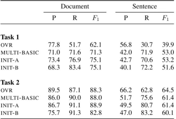
Document Sentence P R F1 P R F1 Task 1 OVR 77.8 51.7 62.1 56.8 30.7 39.9 MULTI-BASIC 71.0 71.6 71.3 42.0 71.9 53.0 INIT-A 73.4 76.9 75.1 42.7 70.6 53.2 INIT-B 68.3 83.4 75.1 40.1 72.2 51.6 Task 2 OVR 89.5 87.1 88.3 66.2 62.8 64.5 MULTI-BASIC 86.0 90.0 88.0 51.7 75.6 61.4 INIT-A 86.7 91.1 88.9 49.5 80.7 61.4 INIT-B 75.7 91.3 82.8 47.0 83.2 60.1

Table 4: Performance results for Tasks 1 and 2. All figures are micro-averages expressed as per-centages.

Table 6 shows the micro-averaged scores across all labels for both tasks.

The results show that for Task 1, all multi-labeled models significantly outperform the OVR model in F1-score, which is explained by a very substantial improvement in recall. INIT-A outper-forms all models in this task, particularly at the document level where there is 5 point improve-ment overMULTI-BASIC.

The results for Task 2 on are more mixed. Over-all, all models achieve a similar F1-score at the

document level. However, there is a clear im-provement in recall at the cost of lower preci-sion when compared to OVR. The best perform-ing model at the document level isINIT-A. On the sentence level,OVRseems to outperform all multi-label models by a good margin. This indicates that the multi-label approach did not aid sentence-level classification in this particular task.

The figures in Table6do not show a complete picture as the interactions between the labels are not taken into account.

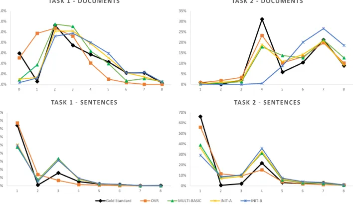
We can observe the proportion of the number of labels assigned to each instance by the classi-fiers, and compare these proportions to the anno-tated gold standard test data. Figure5shows this distribution for each classifier. We can see in Fig-ure5that the overall distributions for all sentence-level classifiers (for both tasks) are closer to the gold standard distribution (compared to document level). This is due to the fact that most sentences have no assigned labels. For Task 2, the classifiers tend to assign more labels than the gold standard.

out-A B C

Figure 4: Illustrating post-processing label correction, with (A) showing the output prediction from the neural network model, (B) applying transitive correction, (C) applying retractive correction.

liers. For Task 1, we observe thatOVR dispropor-tionately assigns exactly one label per document compared to gold standard (where documents have two to three labels on average). In Task 2,INIT-B assigns more labels per document than the gold standard (and every other model).

In addition to looking at the number of labels per class, we also measure the proportion of exact label matches that each model predicts as shown in Table6.

Task 1 Task 2

Doc. Sent. Doc. Sent.

OVR 18.0 67.9 43.4 61.7

MULTI-BASIC 26.2 59.3 40.9 54.2

INIT-A 33.9 65.9 45.6 53.1

INIT-B 31.3 62.6 12.7 49.7

Table 5: The proportion (%) of exact matches. For document classification in Task 1, INIT-A outperforms all models, while OVR significantly underperforms. However, OVR performs signif-icantly better than all other models when classi-fying sentences when considering exact matches only.

Finally, we look at how consistent (well-formed) the predictions output by each model are. We do this by running the post-processing label correction policies described in Section 5.3. Ta-ble6summarizes these results.

For Task 1, OVRshows the largest variance af-ter the application of any method of correction, whereas no multi-labeled model shows this vari-ation. This indicates that the post-processing cor-rections had little effect on the predicted results as they were already well-formed. For Task 2, there is very little variance for all multi-labeled models, with only a slight change forOVR.

Document Sentence O T R O T R Task 1 OVR 62.1 63.9 60.6 39.9 42.2 37.5 MULTI-BASIC 71.3 71.3 71.2 53.0 53.0 53.0 INIT-A 75.1 75.0 75.2 53.2 53.2 53.3 INIT-B 75.1 74.9 75.3 51.6 51.5 51.6 Task 2 OVR 88.3 88.4 88.2 64.5 65.3 63.3 MULTI-BASIC 88.0 87.7 88.1 61.4 61.3 61.7 INIT-A 88.9 88.7 89.0 61.4 61.3 61.5 INIT-B 82.8 82.8 82.8 60.1 59.8 60.4 Table 6: Post-processing label correction. O is the predicted output, T is transitive correction, and R is retractive correction. All figures are micro-averagedF1-scores expressed as percentages.

7 Discussion

The strength of using the hidden-layer initializa-tion for multi-label classificainitializa-tion lies in leverag-ing the co-occurrence between labels. Naturally, if such co-occurrences are relatively rare in the dataset, then this approach becomes less effective. This implies that this approach is especially at-tractive for hierarchical multi-label classification, because of the implicit hypernym–hyponym rela-tions between the labels, which by definition guar-antees co-occurrence of labels in the datasets. The superclass labels must be included when labeling a given example in order to model the hierarchical nature of the labels.

Another key strength of this approach is its low computational cost, which is only proportional to the size of the input text, and the number of label co-occurrences.

However, when there is a large amount of train-ing data, the number of label co-occurrences can be larger than the number of the hidden units. In such a case, one possible option is to select an

ap-02468

Gold Standard OVR MULTI-BASIC INIT-A INIT-B 0.0% 5.0% 10.0% 15.0% 20.0% 25.0% 30.0% 35.0% 0 1 2 3 4 5 6 7 8 TASK 1 - DOCUMENTS 0% 10% 20% 30% 40% 50% 60% 70% 80% 90% 1 2 3 4 5 6 7 8 TASK 1 - SENTENCES 0% 5% 10% 15% 20% 25% 30% 35% 1 2 3 4 5 6 7 8 TASK 2 - DOCUMENTS 0% 10% 20% 30% 40% 50% 60% 70% 1 2 3 4 5 6 7 8 TASK 2 - SENTENCES

Figure 5: The distribution of instances according to the number labels per instance. The number of labels per instance (x-axis), andy-axis is the proportion of instances in the test dataset that have that number of labels. The black line indicates the distribution of the gold standard annotation (i.e.ground truth). propriate subset of label co-occurrences using a

certain criteria such as the frequency in the train-ing data. For the datasets used in this paper, this was not necessary.

Overall, the results of the evaluation show that initializing the model using only label co-occurrences (INIT-A) generally produced a higher performance compared to the other models, in-cluding the random initialization of remaining hid-den units in the final hidhid-den layer (the INIT-B model) as proposed byKurata et al.(2016). How-ever, there was one key exception in Task 2 sen-tence level classification, where the one-vs.-rest OVRmodel achieved the best results.

Both variants of the initialization models in-vestigated here achieved generally positive results when the scope of text is larger (i.e. documents), where there are more labels assigned per text in-stance. However, due to time and computational constraints, this initialization method was not fully utilized as we could only investigate its perfor-mance under a closed set of hyperparamaters for theCNNmodel.

It may be possible for this approach to yield even better results if further parameters are

in-cluded in the CNN models (e.g. more filters and filter sizes). It is also important to note that col-lectively the one-vs.-rest models have much more parameters than any of the the multi-label models in our experiment setup, and therefore they have a higher capacity to capture correlations. In spite of this, the multi-label models have largely outper-formed theOVRmodel.

8 Conclusions

There are many tasks in the biomedical domain that require the assignment of one or more labels to input text. These labels often exists within some hierarchical structure (such as a taxonomy).

The conventional approach is to use a one-vs.-rest classification setup: a binary classifier is trained for each label in the taxonomy or ontol-ogy where all instances not belonging to the class are considered negative examples. The main draw-backs to this approach are that dependencies be-tween classes are not leveraged in the training and classification process, and the additional computa-tional cost of training a classifier for each class.

We applied a new method for multi-label clas-sification that initializes a neural network model

final hidden layer to leverage label co-occurrence. This approach elegantly lends itself to hierarchical classification.

We evaluated this approach using two hierarchi-cal multi-label classification tasks using both sen-tence and document level classification. We use a baseline CNN model with a sigmoid output for each class, and a binary cross-entropy loss func-tion. We investigated two variants of the initial-ization procedure. One used only co-occurrence (and hierarchical information), while the other randomly assigned random values to the remain-ing hidden units in the final hidden layer as pro-posed by Kurata et al.(2016). The experimental results for both tasks show that overall, our pro-posed initialization procedure (INIT-A) achieved better results than all of the the other models, with the exception of sentence-level classification in Task 2, where one-vs.-rest classification attained the best result. We believe that this approach shows promising potential for improving the per-formance for hierarchical multi-label text classifi-cation tasks.

For future work, we plan to try different ini-tialization schemes in addition to the upper bound parameter by Glorot and Bengio(2010) that was used in the paper, and the application of this ap-proach to other tasks and datasets such as Medical Subject headings (MeSH) text classification. Acknowledgements

The first author is funded by the Common-wealth Scholarship Commission and the Cam-bridge Trust. This work is supported by Medical Research Council grant MR/M013049/1 and the Google Faculty Award. We thank Tyler Griffiths for his help in proofreading and editing this paper. References

Simon Baker, Ilona Silins, Yufan Guo, Imran Ali, Jo-han H¨ogberg, Ulla Stenius, and Anna Korhonen. 2016. Automatic semantic classification of scien-tific literature according to the hallmarks of cancer. Bioinformatics32(3):432–440.

Ricardo Cerri, Rodrigo C Barros, and Andr´e CPLF De Carvalho. 2014. Hierarchical multi-label clas-sification using local neural networks. Journal of Computer and System Sciences80(1):39–56. Guibin Chen, Deheng Ye, Erik Cambria, Jieshan Chen,

and Zhenchang Xing. 2017. Ensemble application of convolutional and recurrent neural networks for multi-label text categorization. IJCNN.

Billy Chiu, Gamal Crichton, Anna Korhonen, and Sampo Pyysalo. 2016. How to train good word em-beddings for biomedical NLP. In Proceedings of BioNLP.

Franc¸ois Chollet. 2015. Keras. https://github. com/fchollet/keras.

Wyatt T Clark and Predrag Radivojac. 2013. Information-theoretic evaluation of predicted onto-logical annotations. Bioinformatics29(13):i53–i61. Xavier Glorot and Yoshua Bengio. 2010.

Understand-ing the difficulty of trainUnderstand-ing deep feedforward neural networks. InAistats. volume 9, pages 249–256. Douglas Hanahan and Robert A Weinberg. 2000. The

hallmarks of cancer.Cell100(1):57–70.

Jin-Hyuk Hong and Sung-Bae Cho. 2008. A proba-bilistic multi-class strategy of one-vs.-rest support vector machines for cancer classification. Neuro-computing71(16):3275–3281.

Yoon Kim. 2014. Convolutional neural net-works for sentence classification. arXiv preprint arXiv:1408.5882.

Gakuto Kurata, Bing Xiang, and Bowen Zhou. 2016. Improved neural network-based multi-label classifi-cation with better initialization leveraging label co-occurrence. InProceedings of NAACL-HLT. pages 521–526.

Kristin Larsson, Simon Baker, Ilona Silins, Yufan Guo, Ulla Stenius, Anna Korhonen, and Marika Berglund. 2017. Text mining for improved exposure assess-ment.PloS one12(3):e0173132.

David D Lewis, Yiming Yang, Tony G Rose, and Fan Li. 2004. Rcv1: A new benchmark collection for text categorization research. Journal of machine learning research5(Apr):361–397.

Carolyn E Lipscomb. 2000. Medical subject headings (mesh). Bulletin of the Medical Library Association 88(3):265.

Jinseok Nam, Jungi Kim, Eneldo Loza Menc´ıa, Iryna Gurevych, and Johannes F¨urnkranz. 2014. Large-scale multi-label text classificationrevisiting neu-ral networks. In Joint European Conference on Machine Learning and Knowledge Discovery in Databases. Springer, pages 437–452.

Sampo Pyysalo, Tomoko Ohta, and Sophia Ananiadou. 2013. Overview of the cancer genetics (CG) task of BioNLP Shared Task 2013. InBioNLP Shared Task 2013 Workshop.

Artem Sokolov and Asa Ben-Hur. 2010. Hierarchi-cal classification of gene ontology terms using the gostruct method. Journal of bioinformatics and computational biology8(02):357–376.

Artem Sokolov, Christopher Funk, Kiley Graim, Karin Verspoor, and Asa Ben-Hur. 2013. Combin-ing heterogeneous data sources for accurate func-tional annotation of proteins. BMC bioinformatics 14(3):S10.

Aixin Sun and Ee-Peng Lim. 2001. Hierarchical text classification and evaluation. InData Mining, 2001. ICDM 2001, Proceedings IEEE International Con-ference on. IEEE, pages 521–528.

Min-Ling Zhang and Zhi-Hua Zhou. 2006. Multilabel neural networks with applications to functional ge-nomics and text categorization. IEEE transactions on Knowledge and Data Engineering18(10):1338– 1351.