Contents lists available at ScienceDirect
Data
in
Brief
journal homepage: www.elsevier.com/locate/dib
Data Article
Land
cover
maps
of
Antananarivo
(capital
of
Madagascar)
produced
by
processing
multisource
satellite
imagery
and
geospatial
reference
data
Dupuy
Stéphane
a ,c ,d ,∗,
Defrise
Laurence
b ,c ,d,
Gaetano
Raffaele
c ,d,
Andriamanga
Valérie
b,
Rasoamalala
Eloise
baCIRAD,UMRTETIS,F-97410Saint-Pierre,Réunion,France bCIRAD,UMRTETIS,101,Antananarivo,Madagascar cCIRAD,UMRTETIS,F-34398,Montpellier,France
dTETIS,AgroParisTech,CIRAD,CNRS,INRAE,UnivMontpellier,Montpellier,France
a
r
t
i
c
l
e
i
n
f
o
Articlehistory:
Received 24 June 2020 Accepted 26 June 2020 Available online 30 June 2020
Keywords:
Remote sensing Land cover map Spatial database Landsat-8 Sentinel-2 Pleiades OBIA Antananarivo
a
b
s
t
r
a
c
t
Wedescribeareferencespatialdatabaseand fourlanduse mapsofAntananarivocityproducedover2017referenceyear using amethodologycombining machinelearning and ob-jectbasedimageanalysis (OBIA).Thesemapsareproduced byprocessingsatelliteimagesusingtheMoringalandcover processingchaindevelopedinourlaboratory.Weusea sin-gleveryhighspatialresolution(VHSR)Pleiadesimage,atime seriesofSentinel-2and Landsat-8images, aDigitalTerrain Model (DTM) and the aforementioned reference database. According to the Moringa workflow, the Pleiades image is used to generate a suitable object layer at VHSR using a segmentation algorithm. Each object is then classified us-ingvariablesfromthetimeseriesandinformationfromthe DTM. The reference database used to train the supervised classification algorithmis here described, as well as the 4 land cover maps produced at four different hierarchically nested nomenclaturelevels. Fora number ofclasses going from2to20,overallaccuraciesrangefrom94%to74%.Such
∗ Corresponding author at: CIRAD, UMR TETIS, F-97410 Saint-Pierre, Réunion, France.
E-mailaddress:[email protected] (D. Stéphane). https://doi.org/10.1016/j.dib.2020.105952
2352-3409/© 2020 The Authors. Published by Elsevier Inc. This is an open access article under the CC BY license. ( http://creativecommons.org/licenses/by/4.0/)
2 D.Stéphane,D.LaurenceandG.Raffaeleetal./DatainBrief31(2020)105952
landcoverproductsareveryrareinMadagascar,sowehave decidedtomakethemopenlyaccessibleandusablebyland managersandresearchers.
© 2020TheAuthors.PublishedbyElsevierInc. ThisisanopenaccessarticleundertheCCBYlicense. (http://creativecommons.org/licenses/by/4.0/)
Specificationstable
Subject Computer Science, Earth Sciences, Social Sciences Specific subject area Remote Sensing, GIS, Land Cover Map
Type of data Vector How data were
acquired
The reference database was created with the QGIS software ( www.qgis.org) For the production of land use maps, the Moringa processing chain uses the Orfeo ToolBox software ( www.orfeo-toolbox.org) driven by Python scripts. The source code of the Moringa processing chain is available at
https://gitlab.irstea.fr/raffaele.gaetano/moringa.git Data format Raw data (Shapefile, Esri)
Parameters for data collection
To build the reference database, plots were chosen in order to have (i) a good
representativeness of each class and (ii) a homogeneous distribution of classes over the study area
Description of data collection
To build the reference database, GPS waypoints were collected during the end of 2017 rainy season. A Trimble Yuma2 tablet was used to collect the waypoints. Each waypoint was then converted into a polygon by digitizing the boundaries of the corresponding land cover using the VHSR Pleiades image as a support for photo-interpretation. To produce the land use maps, the Moringa processing chain was used, implementing aa supervised classification method for satellite images (Sentinel2, Landsat8 and Pleiades) based on the Random Forest algorithm driven by the reference database mentioned above. We produced four land use maps using the reference database and satellite image classifications as described below.
Data source location Antananarivo, capital of Madagascar located in the Indian Ocean (upper left corner: 18 °43 37.71 ’S and 47 °19 23.42 ’E // lower right corner: 19 °06 07.73 ’S and 47 °39 14.21 ’E)
Data accessibility Repository name: CIRAD Dataverse Data identification number:
Land Use Map: Dupuy, Stéphane; Defrise, Laurence; Gaetano, Raffaele; Burnod, Perrine, 2019, "Antananarivo - 2017 Land cover map", doi:10.18167/DVN1/NHE34C, CIRAD Dataverse, V2
Reference database: Laurence, Defrise; Andriamanga, Valérie; Rasoamalala, Eloise; Dupuy, Stéphane; Burnod, Perrine, 2019, "Antananarivo - Madagascar - 2017, Land use reference spatial database", doi:10.18167/DVN1/5TZOOW, CIRAD Dataverse, V1 Direct URL to data:
Data are referenced in the CIRAD Dataverse and are hosted on CIRAD’s Aware Geographic catalog. The web links are in the following files.
Land use map: http://dx.doi.org/10.18167/DVN1/NHE34C Reference database: http://dx.doi.org/10.18167/DVN1/5TZOOW
Related research article S. Dupuy, L. Defrise, V. Lebourgeois, R. Gaetano, P. Burnod, J.-P. Tonneau, analyzing Urban Agriculture’s Contribution to a Southern City’s Resilience through Land Cover Mapping: The Case of Antananarivo, Capital of Madagascar, Remote Sensing. 12 (2020). https://doi.org/10.3390/rs12121962.
Valueofthedata
• Themapscanbeusedbyinstitutionsandlandplannerstoupdateurbanandsanitation mas-terplans.
• Thereferencedatabasecanbeusedbyremotesensingspecialiststoassessnewmethodsfor landcovermappingandotherclassificationalgorithms.
Table1
Nomenclature presenting the four levels of precision and the number of polygons in reference database level 4. Level 1
Crop Land
Level 2 Land Cover Level 3 Crop Group Level 4 Crop Class Number of polygons
Non crop Urban area Built-up surface Mixed habitat 284
Residential area 149
Rural housing 110
Industrial, commercial and military area
Industrial, commercial and military area
99 Quarry, landfill and
construction site
Quarry, landfill and construction site
60
Brick extraction 111
Natural spaces Bare non-agricultural soil
Bare non-agricultural soil 87
Savannah Herbaceous savannah 111
Shrub savannah 155
Forest Forest Tree savannah 196
Pines 110
Waterbodies and wetland
Water bodies Water bodies 143
Wetland Wetland 80
Crop Annual and pluriannual crops
Irrigated crop Rice 350
Watercress 83
Vegetable crop Vegetable crop 371
Rainfed crop Cassava 192
Other rainfed crop 140
Fallows, pasture and agricultural bare soil
Fallows, pasture and bare agricultural soil
Fallows, pasture and bare agricultural soil
99
Fruit crop Fruit crop Fruit crop 138
TOTAL 3 068
1. Datadescription
Thedatadescribedinthispaperareoftwodifferenttypesrelatedtolanduseonthegreater Antananarivoarea:
• AGISreferencedatabaseinESRIshapefileformatcomposedof3068polygonsrepresentative ofthediversityoflandusesinAntananarivo.Eachpolygonisannotatedwithfourclasslabels correspondingtofourlevelsofnomenclature.Classnomenclaturesarehierarchicallynested, and the number of classes ranges from 2 atlevel 1 (crop vs. non-crop) to 20 at level 4. Detailed hierarchicalnomenclature is shownin Table 1 . Thisdatabase is used to generate trainingsamples in theMoringa supervised classification process in orderto identify land useclassesfromasetofvariablesextractedfromhighandveryhighspatialresolution satel-lite images.We usethe reference database to evaluate the accuracy of the provided land usemapswithacross-validationtechnique.Thespatialdistributionofreferencepolygonsis depictedin Fig. 1 .
• Fourlandusemapsproducedby processingmultisourcesatellite dataincludingaVeryHigh SpatialResolution(VHRS)Pleiadesimage,atimeseriesofHRSSentinel-2andLandsat-8 im-agesanda digitalterrain model.Eachmapcorrespondtolanduseatoneofthefourlevels ofnomenclature(from2to20classes),andisdistributedinvectorformat(shapefile).Each geometrycorresponds toanobjectprovidedbythesegmentation ofthePleiadesimage, at-tributedusinga classlabelatthe specificnomenclature level.Validationresultsshow that mapaccuraciesrangefrom76%forthemostdetailednomenclaturelevel(20classes)to94% fortheleastdetailedlevel(2classes).Thefourmapsproducedareillustratedin Figs. 2 –5 . FinalmapsinESRIshapefileformataredeliveredinthelocalUTMprojection (WGS84UTM 38South,EPSGcode32,738).DataarereferencedintheCIRADDataverse.Furtherdescriptionof thesedataandtheiruseinarealworldcasestudyisdetailedinthearticle [1] .
4 D.Stéphane,D.LaurenceandG.Raffaeleetal./DatainBrief31(2020)105952
Fig.1. Distribution of the collected polygons - Vector file in ESRI shape format available here: http://dx.doi.org/10.18167/ DVN1/5TZOOW.
2. Experimentaldesign,materials,andmethods
2.1. Materials
2.1.1. 2017referencedatabaseandnomenclature
The referencedatabase is organizedaccording to a multi-levelnomenclature (Cf. Table 1 ). Fieldsurveyswereperformedduringtheendofthe2017rainyseason(MarchtoApril), which correspondstothepeakofthegrowingseason.GPSwaypointswere collectedfollowingan op-portunisticsamplingapproach [2] .Waypointswerecollectedwithinthewholestudyareain or-dertohavearepresentativenessoftheexistingtypesofcropsandurbanstructures.GPSpoints havealsobeenrecorded foruncultivatedandunbuiltplots such assavannah, forest ormarsh. Eachwaypoint was then converted into a polygon by digitizing the boundariesof the corre-spondinglandcoveron aVHSRPleiadesimage (0.5m∗ 0.5mpixelsize). 981additional poly-gonsweredigitizedbyphotointerpretationofthePleiadesimage foreasilyrecognizableclasses (housing,brickextraction,rice, watercressandsavannah). Thefinal grounddatabasewasthus composedof3068polygons(Cf. Fig. 1 ).
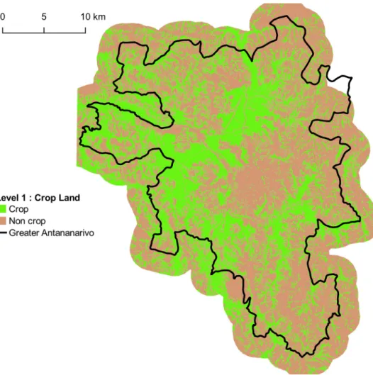
Fig.2. Land cover map corresponding to Level-1 with 2 classes. Vector file in ESRI shape format available here: http: //dx.doi.org/10.18167/DVN1/NHE34C. This figure is a modified version of Fig.5 published in this article [1].
2.1.2. Images
➢ VeryHighSpatialResolution(VHSR):
Two20×20kmPleiadestiles(withspatialresolutionof2mand0.5m)wereacquired simul-taneously on January 8, 2017,which corresponds to the middleof therainy season in Mada-gascar. Pleiades images were acquired with the support of CNES (Centre National d’Etudes Spatiales: government agency responsible for shaping and implementing France’s space pol-icy in Europe). Pleiades images are not free and are available under condition of eligibility via theTheia consortium(DataandServicescentreforcontinental surfaces)andtheDINAMIS programme. More information is available on the Theia website (https://www.theia-land.fr/ le- programme- isis- du- cnes- sintegre- a- dinamis ).
➢ HighSpatialResolution(HSR):
TheHighSpatialResolutiontimeseriesconsistsof50imagesacquiredbetweenOctober2016 andSeptember2017(including19imagesfromLandsat-8and62imagesfromSentinel-2(2tiles and31acquisitiondates)).Selectioncriteriafortheseimageswere:imagesshouldcoveratleast 20%ofthestudyareaandhavelessthan80%cloudcoverpertile.
6 D.Stéphane,D.LaurenceandG.Raffaeleetal./DatainBrief31(2020)105952
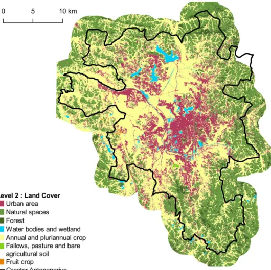
Fig.3. Land cover map corresponding to Level-2 with 8 classes. Vector file in ESRI shape format available here: http: //dx.doi.org/10.18167/DVN1/NHE34C. This figure is a modified version of Fig.5 published in this article [1].
TheSentinel2Aand2Bsatellites(S2AandS2B)havebeendeployedbytheEuropeanSpace Agency(ESA). The imagesoffer 13 spectral bandswitha spatialresolutionbetween10m and 60m.Theintervalbetweentwosubsequentacquisitionsis5daysconsideringbothsatellites.In thisstudy,Sentinel-2(S2)level-1CimagesprovidedbyESAwere usedandonly10bandswere keptwitharesolutionof10mand20m.
TheLandsat-8(L8)satellitewasdeployedbytheNationalAeronauticsandSpace Administra-tion(NASA).Therevisitingfrequencyis16days.L8imageshaveaspatialresolutionof15mfor thepanchromaticbandand30mforthemultispectralbands.
The characteristics of the L8 andS2 images are different, but in tropical areas with high cloud cover,the combinationof thesesensors increasesthe probability of regularly observing theentireterritory.
2.1.3. Topography
TheShuttle RadarTopography Mission(SRTM) digital elevationmodel (DEM) at30m spa-tial resolution was downloaded from United States Geological Survey (USGS) website (https: //earthexplorer.usgs.gov )totakeintoaccountthetopography(altitude,slope)ofthestudyzone.
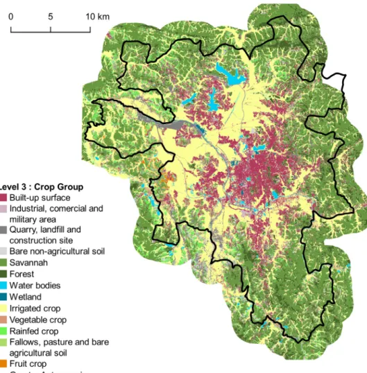
Fig.4. Land cover map corresponding to Level-3 with 13 classes. Vector file in ESRI shape format available here: http: //dx.doi.org/10.18167/DVN1/NHE34C.
2.2. Moringaprocessingchaintoobtainlandcovermapin2017
The Moringa processing chain was used to automate the production of land cover maps at Very High Spatial Resolution (VHSR) following a methodology that is particularly adapted to tropicalagricultural systems(cloudy acquisitions,smallfield sizes, heterogeneous and frag-mented landscapes)[3 ,4 ]. The Moringa chaincan be downloadedat thefollowing link: https: //gitlab.irstea.fr/raffaele.gaetano/moringa
The methodology is based on the combined use of Very High Spatial Resolution (VHSR) Pleiades imagery, time seriesof Sentinel-2 andLandsat-8 High Spatial Resolution (HRS) opti-cal imagesand a Digital Terrain Model (DTM) within an Object Based Image Analysis (OBIA) and Random Forest classification approach driven by a referencedatabase combining in situ andphoto-interpretation measurements.The chainisbuiltupon theOrfeo Tool Box(OTB) ap-plications,drivenbypythonscripts.Somepre-processingstepsareperformedunderQGiS.Main processesofthechainaresummarizedin Fig. 6 .Thefollowingparagraphsdescribespecific pa-rametersandusefulelementsoftheclassificationmethod.
8 D.Stéphane,D.LaurenceandG.Raffaeleetal./DatainBrief31(2020)105952
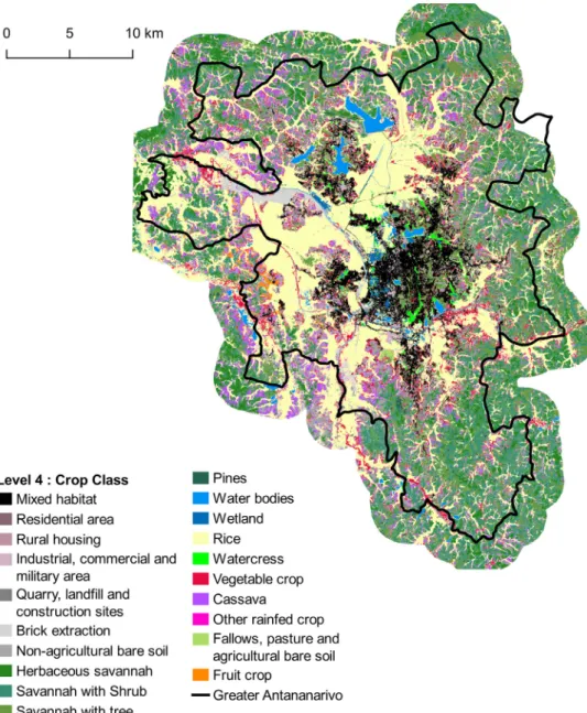
Fig.5. Land cover map corresponding to Level-3 with 20 classes. Vector file in ESRI shape format available here: http: //dx.doi.org/10.18167/DVN1/NHE34C. This figure is a modified version of Fig.5 published in this article [1].
2.2.1. VHSRpre-processing
Preprocessing steps were realized with Orfeo ToolBox [5] and consisted in Top of Atmo-sphere(TOA) reflectance calculation,andorthorectification ofPleiade image.Orthorectification ofpanchromaticandmultispectralimageswasbasedonSRTMdigitalelevationmodelandthe “Orthobase Madagascar” product (orthorectified mosaic of 2.5m panchromatic SPOT5 images wasacquiredtoserve asa referencefortheco-registration ofPleiades images). Theseimages are available underthe conditionof eligibility distributedby SEAS-OI (Survey ofthe Environ-ment Assisted by Satellite in the Indian Ocean): http://www.seas-oi.fr . The two PAN andMS
10 D.Stéphane,D.LaurenceandG.Raffaeleetal./DatainBrief31(2020)105952
Table2
Description of variables extracted to compute the classification (with HSR = High Spatial Resolution and VHSR = Very High Spatial Resolution). This table is a modified version of Table2published in this article [1].
Type HSR VHRS Topography
Spectral reflectance
Landsat-8: 7 bands and Sentinel-2: 10 bands
Spectral indices NDVI 1[7], MNDVI 2[8], NDWI 3[9],
MNDWI 4[10], brightness index 5and
RNDVI 6[11]
Textural indices Energy, Contrast et
Variance Haralick indices [12]calculated at 2 windows size: 5 ×5 and 11 ×11
Topographic indices
Altitude and slope
number 1024 6 2
1: Normalized Difference Vegetation Index. 2: Modified Normalized Difference Vegetation Index. 3: Normalized Differ- ence Water Index. 4: Modified Normalized Difference Water Index. 5: Square root of the sum of squared values of all bands. 6: Rededge NDVI (only for Sentinel-2).
tileswerethenmosaickedandtheresultedmosaicswere pansharpenedusingtheBayesian fu-sionalgorithmofthe OTB pansharpeningmodule inordertoobtain amultispectral mosaicat 0.5mspatialresolution.
2.2.2. HSRpre-processing
Pre-processingappliedtoHRSimagesisautomatedintheMoringachain:
• The62Sentinel-2tilesweremosaickedtoproduceatimeseriesof31mosaics.
• FortheLandsat-8pansharpeningprocessingisappliedtobringthespatialresolutionasclose aspossibletoS2images.
S2andL8imageswerecoregisteredtotheVHSRPleiadesreferenceusinganautomatic pro-cedure basedonthe homologouspointsextractionapplicationof OTB.Thisprocessing is con-ceived toimprove overlapping among thedifferent remote sensingsources, and iscrucial for thecharacterizationofsmallscaleobjects.
Fmasktool [6] wasusedtoproducethecloudmaskscorrespondingtoeachimageofthetime series.The chainproduces, fromthecloud masks,an image illustratingthenumberoftimesa pixelisnotcoveredbycloudsinthetimeseries.Thisillustrationlocatestheareaswherethere isariskofinstabilityoftheresultsonthemapsifthenumberofclearacquisitionsislow(Cf. Fig. 6 ).
2.2.3. Thevariablesusedintheclassification
➢ 6commonradiometricindicesusefulforlandusecharacterizationwerechosen(Cf. Table 2 ) ➢ TexturesareimportanttodetectvisiblepatternsontheTHRSimagesuchastreealignments inagricultural crops.In theMoringa chain,thesetextureindices aretheonly variables de-rived fromtheVHSRimage.The OTB"HaralickTextureExtraction"algorithmwasusedand appliedtothepanchromaticimage(Cf. Table 2 )
➢ Slopes were calculated using QGIS software. DTM andslopes are used as variables in the classificationprocess.
2.2.4. Objectbasedclassification
TheMoringa processingchainisdesignedto provideobject-basedsupervisedclassification, andoperatesbyfirstperformingthesegmentationoftheVHSRimagetogenerateasuitable ob-jectlayer.Themethoddescribedin [13] ,implementedinthelargescaleversionofOTB’s Gener-icRegionMergingapplication [14] ,wasusedtoperform thesegmentation.Toobtain a segmen-tationresultadapted toourstudy,parameters forthehomogeneitycriteriaandthemaximum
D. St ép h a n e, D. Laur ence and G. Ra ffa el e et al. / Dat a in Brief 31 (2020) 105952 11
Globalandclassaccuracyindicesbylevel.ThistableisamodifiedversionofTable4publishedinthisarticle[1].
LEVEL1 F1-SCORE LEVEL2 F1-SCORE LEVEL3 F1-SCORE LEVEL4 F1-SCORE
Noncrop 96.13% Urbanarea 91.6% Built-upsurface 83.5% Mixedhabitat 65.1%
Residentialarea 8.2%
Ruralhousing 52.8%
Industrial,commercialand militaryarea
81.8% Industrial,commercialand
militaryarea
84.1% Quarry,landfilland
constructionsite
86.8% Quarry,landfillandconstruction
site
68.0%
Brickextraction 94.7%
Naturalspaces 73.1% Barenon-agriculturalsoil 41.8% Barenon-agriculturalsoil 44.9%
Savannah 75.6% Herbaceoussavannah 62.4%
Shrubsavannah 58.4%
Forest 86.8% Forest 86.9% Treesavannah 63.0%
Pines 63.0%
Waterbodiesandwetland 90.4% Waterbodies 97.5% Waterbodies 97.4%
Wetland 61.9% Wetland 70.2%
Crop 91.7% Annualandpluriannualcrop 88.5% Irrigatedcrop 89.1% Rice 88.0%
Watercress 78.3%
Vegetablecrop 37.1% Vegetablecrop 41.1%
Rainfedcrop 47.4% Cassava 48.6%
Otherrainfedcrop 0%
Fallows,pastureandbare agriculturalsoil
63.7% Fallows,pastureandbare
agriculturalsoil
66.8% Fallows,pastureandbare
agriculturalsoil
67.7%
Fruitcrop 45.0% Fruitcrop 68.% Fruitcrop 67.7%
Overallaccuracy 94.78% 86.83% 84.08% 76.56%
12 D.Stéphane,D.LaurenceandG.Raffaeleetal./DatainBrief31(2020)105952
heterogeneitythresholdwere assessedusinga gridsearch onseveralrepresentativesubsetsof theVHSRpansharpenedimage.Thefollowingparameterswerefinallychosen:
➢ Scaleparameter:150 ➢ Shapeparameter:0.3 ➢ Compactnessparameter:0.7
Trainingsamplesweresubsequentlygeneratedbyintersectingtheso-obtainedsegmentation withthereferencepolygonsavailableintheGISdataset,andattributedusingthespatialmeans overeveryband andindexlistedin Table 2 .RandomForest (RF)classificationalgorithm[14 ,15 ] waschosenforclassificationconsideringitsrobustnesswhenworkingwithheterogeneousdata, such as in our study (data from several sensors combined with altitude, slopes and textural indices).
AnindependentRFmodelwasbuiltforeachnomenclaturelevel,andappliedforthe classifi-cationofthewholesetofobjects,whichwerebeforehandattributedinthesamewaydescribed forthetrainingsamples.At theendoftheprocess,thefourlandusemapsare madeavailable invectorandrasterformat.
2.2.5. Validationof2017maps
Wehereusethe k-foldcross-validationtechniqueto evaluatethe accuracyoftheprovided land use maps.The specific validation protocol(number of folds, accuracy metrics)for these mapsisthesamealreadyusedin[1 ,4 ]
Thesequalityindicators(globalaccuracy,Kappa,fscore)aregivenin Table 3 . 2.2.6. Smoothingbymajorityfilter
Amajorityfilterwasapplied totherasterizedclassificationtosmoothout contoursand re-move isolated pixels. OTB’s Classification Map Regularization tool was used. The size of the structuring element can be adjusted to measure the intensity of the smoothing. Tolimit the degradationoftheclassification,afilterofradius1,corresponding toa3×3pixelwindow,was chosen.
DeclarationofCompetingInterest
Theauthorsdeclarethattheyhavenoknowledgeofcompetingfinancialinterestsorpersonal relationshipswhichhave,orcould be perceived tohave, influencedthe workreported inthis article.
Acknowledgments
ThisworkwassupportedbyafinancialcontributionfromCiradandINRAEwiththeGlofood meta-programme(LEGENDEproject).
Thiswork wassupported by afinancial contributionfrom theEuropean Regional Develop-mentFund(EuropeanUnion),theFrenchStateandtheReunionRegion.
Thiswork benefited fromthe Pleiades images of the French CNES DINAMISprogram help (ISIS).
ThisworkbenefitedfromagrantfromAgroParisTechABIESdoctoralschool.
Supplementarymaterials
Supplementarymaterial associated withthisarticlecan be found,inthe onlineversion, at doi:10.1016/j.dib.2020.105952 .
References
[1] S. Dupuy, L. Defrise, V. Lebourgeois, R. Gaetano, P. Burnod, J.-.P. Tonneau, Analyzing urban agriculture’s contribution to a Southern City’s resilience through land cover mapping: the case of Antananarivo, capital of Madagascar, Remote Sens. (2020) 12 https://doi.org/, doi: 10.3390/rs12121962.
[2] V. Lebourgeois, S. Dupuy, É. Vintrou, M. Ameline, S. Butler, A. Bégué, A combined random forest and OBIA classifica- tion scheme for mapping smallholder agriculture at different nomenclature levels using multisource data (simulated sentinel-2 time series, VHRS and DEM), Remote Sens. (2017) 9 https://doi.org/, doi: 10.3390/rs9030259.
[3] R. Gaetano, S. Dupuy, V. Lebourgeois, G. Le Maire, A. Tran, A. Jolivot, A. Bégué, in: The MORINGA Processing Chain: Automatic Object-Based Land Cover Classification of Tropical Agrosystems Using Multi-Sensor Satellite Imagery, Ital- ian Space Agency, Milan, Italie, 2019, p. 3. http://agritrop.cirad.fr/594650/1/Living%20Planet_abstract2019_Gaetano. pdf.
[4] S. Dupuy, R. Gaetano, L. Le Mézo, Mapping land cover on Reunion Island in 2017 using satellite imagery and geospa- tial ground data, Data Brief 28 (2020) 104934 https://doi.org/, doi: 10.1016/j.dib.2019.104934.
[5] Jordi Inglada, Emmanuel Christophe, The Orfeo Toolbox remote sensing image processing software, in: Proceedings of the IEEE International Geoscience and Remote Sensing Symposium, 2009, pp. IV–733, doi: 10.1109/IGARSS.2009. 5417481. https://doi.org/.
[6] S. Qiu, Z. Zhu, B. He, Fmask 4, Improved cloud and cloud shadow detection in Landsats 4–8 and Sentinel-2 imagery, Remote Sens. Environ. 231 (2019) 111205 https://doi.org/, doi: 10.1016/j.rse.2019.05.024.
[7] J.W. Rouse Jr., R.H. Haas, J.A. Schell, D.W. Deering, Monitoring Vegetation Systems in the Great Plains With ERTS, Remote Sensing Center, Texas A&M University, College Station, Texas, 1974 https://ntrs.nasa.gov/archive/nasa/casi. ntrs.nasa.gov/19740022614.pdf.
[8] C. Jurgens, The modified normalized difference vegetation index (mNDVI) a new index to determine frost damages in agriculture based on Landsat TM data, Int. J. Remote Sens. 18 (1997) 3583–3594 https://doi.org/, doi: 10.1080/ 014311697216810.
[9] B. Gao, NDWI—A normalized difference water index for remote sensing of vegetation liquid water from space, Re- mote Sens. Environ. 58 (1996) 257–266 https://doi.org/, doi: 10.1016/S0034-4257(96)00067-3.
[10] H. Xu, Modification of normalised difference water index (NDWI) to enhance open water features in remotely sensed imagery, Int. J. Remote Sens. 27 (2006) 3025–3033 https://doi.org/, doi: 10.1080/01431160600589179. [11] C. Schuster, M. Förster, B. Kleinschmit, Testing the red edge channel for improving land-use classifications based on
high-resolution multi-spectral satellite data, Int. J. Remote Sens. 33 (2012) 5583–5599 https://doi.org/, doi: 10.1080/ 01431161.2012.666812.
[12] R.M. Haralick, K. Shanmugam, I. Dinstein, Textural Features for Image Classification, IEEE Transactions on Systems, Man, and Cybernetics, SMC-3 (1973) 610–621 https://doi.org/, doi: 10.1109/TSMC.1973.4309314.
[13] M.Baatz,in:MultiResolutionSegmentation:anOptimumApproachForHighQualityMultiScaleImage Segmenta-tion,2000,BeutrageZumAGIT-Symposium,Salzburg,Heidelberg,2000,pp.12–23.
[14] P.Lassalle, J.Inglada,J.Michel,M.Grizonnet,J.Malik,Largescaleregion-mergingsegmentationusingthelocal mutualbestfittingconcept,in:ProceedingsoftheIEEEGeoscienceandRemoteSensingSymposium,IEEE,2014, pp.4887–4890.