UNIVERSITY OF TARTU
Institute of Computer Science
Curriculum
Toria Ketevan
Predicting Academic Performance From
Admission Scores and Application Data –
A Case Study
Master’s Thesis (30 ECTS)
Supervisor(s): Marlon Dumas, Irene-Angelica Chounta
Predicting Academic Performance From Admission Scores and Application Data – A Case Study
Abstract:
During the admissions process at the University of Tartu’s Master's programme, students get an admission score, which is calculated based on their motivation letter and their Bachelor’s Grade Point Average (GPA). Ideally, the admission score should be predictive of student’s academic performance during their Master's studies. Hence, one would expect that the higher the admission score is, the better is the academic performance of the candidate once they join the Master's program. However, this hypothesis has not been tested in the context of University of Tartu's admission process. In this thesis, we evaluate the efficiency of the admission score and produce more accurate and reliable student’s academic performance prediction model by analysing the application documents using data mining techniques.
Keywords:
educational data mining, academic performance prediction, admission score, classification model, feature selection algorithms
CERCS: P175
Akadeemiliste tulemuste ennustamine sisseastumispunktide ja - avalduste põhjal - juhtumiuuring
Lühikokkuvõte:
Tartu Ülikooli magistriõppesse vastuvõtmisprotsessi käigus saavad tudengid punktid, mis arvutatakse välja nende motivatsioonikirja ja bakalauseuseõppe keskmise hinde alusel. Ideaalis peaksid sisseastumispunktid ennustama tudengi akadeemilisi tulemusi magistriõppes, mistõttu võib eeldada, et mida kõrgemad on sisseastumispunktid, seda paremad on kandidaadi akadeemilised tulemused pärast magistriõppesse astumist. Seda hüpoteesi pole aga Tartu Ülikooli vastuvõtmisprotsessi kontekstis testitud. Selles lõputöös hinnatakse sisseastumispunktide efektiivsust ning koostatakse täpsem ja usaldusväärsem tudengite akadeemiliste tulemuste prognoosimismudel, analüüsides sisseastumisdokumente andmekaevandamise metoodikate abil.
Võtmesõnad:
sisseastumislävend, hariduslik andmete hankimine, akadeemilise edukuse prognoos, klassifitseerimise mudel, tunnuste valimise algoritm
CERCS: P175
Table of Contents
1. Introduction 5
2. State of the art 10
3. Methodology 12
3.1. Methods 12
3.1.1 DreamApplyParser 12
3.1.2. Data mining tools 13
3.2. Data 13
3.2.1. Construction of the dataset 13
3.2.2. Transform data 16
3.2.3. Data clean and imputation process 16
3.2.4. Non-numeric values into numeric 16
3.2.5. Variable Types 17
4. Analysis/Results 20
4.1. Analysis of the existing model 20
4.2. Feature selection 24
4.3. Academic performance prediction model 30
4.3.1. Selecting classification algorithms 31
4.3.2. Naive Bayes 31 4.3.3. Random forest 34 5. Conclusion 38 5.1. Future improvements 38 6. Bibliography 39 4
1.
Introduction
Admission is the process through which students get enrolled in universities and colleges. Admission processes (AP) vary widely from country to country, and sometimes even from institution to institution. Nowadays, students can apply to an institution by submitting application forms online. After collecting and processing the data, educational stakeholders accept or decline the students based on different criteria. In this paper we are assuming that the universities accept students that they believe will show better performance, in terms of grades, then others. This should be the case for most, if not all of the universities, since according to this survey [4] "By one-point increase in a person's high school GPA, average annual earnings in adulthood increased by about 12 percent for men and about 14 percent for women" and successful graduates increase the university's reputation. Thus, to make a decision whether or not to accept the candidate, educational institutions have developed student performance prediction models which help them predict student's potential performance in that educational institution. Hence, having an effective performance prediction model is very important for an educational institution.
Educational institutions store various data related to student’s activities in educational settings. Apart from grades, it can include much more detailed and comprehensive information about student’s learning activities. For example, some online learning management systems (LMS) also track and store information such as how many times the exercise was repeated, how long was student thinking about each question and so on. These data are usually called educational data. By analysing the educational data, we can find interesting patterns which help to build effective student performance prediction models. However, doing such analysis is not a new practice. It is part of the so-called Educational Data Mining (EDM). EDM is an interdisciplinary field bringing together researchers from computer science, education, psychology, psychometrics, and statistics to analyze large data sets to answer educational research questions [3].
In Figure 1, we can see the visualisation of data mining applied to educational systems. As we can see from the picture, all of the participants of the education process are part of the cycle: Educators and responsible academics build and maintain the educational systems, while students interact with them. Result of those interactions, including academic data and other useful interaction data are gathered and data mining techniques are applied to it. Those techniques can be oriented to students and can be used to recommend various resources and activities that would improve their performance or make student’s performance predictions. Data mining techniques can also be oriented towards educators and can be used to evaluate the effectiveness of the learning process and to discover how it can be improved, for example by restructuring groups of students or increasing frequency of some activities that are more effective.
However, applying machine learning methods on educational data for building student performance prediction models has its difficulties. The original data contain numerous irrelevant and redundant information. These redundant data might affect the results of prediction[1]. Students academic performance hinges on diverse factors or characteristics such as demographics, personal, educational background, psychological, academic progress and other environmental variables. The interrelationship between these variables participating in the complex and multi-faceted problem of academic performance are not clearly understood, and they are often related in a complicated nonlinear way [2]. Other than that, educational data come from different sources and the data size is also different for each educational institution. The performance of machine learning methods is heavily dependent on the choice of data representation and the size of the dataset. That being said, there is no single approach which is effective for all the institutions to predict student academic performance.
This thesis focuses on improving the admission process at the University of Tartu. The University of Tartu (UT) is a classical university in the city of Tartu, Estonia. It is the only classical university in the country. According to Wikipedia, it is also the biggest and the most prestigious university in Estonia. There are nearly 14,000 students at the university, of which over 1,300 are foreign students.
The admission process at UT is the following. Admission applications are extracted from the student admission management system called Dreamapply . Next step is to1 check the diploma and find the final GPA in the diploma images. Diplomas come from different countries and look different which makes it a difficult process. Apart
1https://estonia.dreamapply.com/
from that, universities have different grading systems. From our previous experience, in most cases, it is country related. For example, universities from some countries have grades from 1 to 5 and 1 is the highest, while others grade from 1 to 4 and 4 is the highest. In order to be able to compare applicants, normalization of GPA scores is needed and this process is done very carefully. Normalization is done by converting the original GPA to number from 1 to 100. The following step of the admission process is to validate and score motivation letters. For validating motivation letters automatic text-recognition system tool called Urkund is used.2 Urkund tool gives the percentage of plagiarized text for each motivation letter. Finally, University professors check motivation letters and assign a score from 1 to 100. The final admission score of the applicant is calculated as a weighted sum of motivation letter score and normalized GPA with weights 2 and 3 and then normalizing back to score from 1 to 100. The admission offer is made based on this admission score.
Ideally, the admission score should be predictive of the future academic performance of the student. In other words, a higher admission score should be associated with higher academic performance. However, this hypothesis has not been tested in the context of the University of Tartu's admission process.
To evaluate the effectiveness of the admission process at the University of Tartu, we should study the correlation between the admission score and the final GPA. That being said, the first question of this research is: To what extent this admission score is correlated with student’s actual academic performance?
In this study we have collected the admission data for the years 2013 to 2018 for students who have applied for Software Engineering program at the University of Tartu. After data preparation, we decided to calculate the Pearson's correlation coefficient to find out the correlation between admission score and actual student performance. The correlation turned out to be positive but not strong, which meant that there might be a space for improvement. To expand on this, we wanted to detect, besides GPA and motivation letter, if there were other useful features such as demographics, personal, educational background and other environmental variables which affect student performance in UT. For example, the percentage of plagiarized text in motivation letter could also be a useful setting for student’s performance prediction. Other than that, It is relatively hard to get high grades in some universities compared to the other ones. This means that, apart from GPA we also might consider the university itself. For this purpose, it would be great to have some sort of ranking of the universities as a separate feature.
This leads us to our second research question: To what extent, machine learning techniques can be used to produce a more accurate and reliable admission score by automatically analyzing the admission application documents?
2https://www.urkund.com
Before we could do the analysis we had to collect the data. As mentioned earlier, UT uses student admission management system called DreamApply. We automated extraction of data from DreamApply by developing a software tool called DreamApplyParser, which authenticates into Dreamapply system, removes personal identifiers, extracts applicant’s data except GPA and exports it in CSV format. It also gives the ability to filter applicants by program name and generates .txt files for motivation letters. In order to extract GPA we would need to process diploma images which is very hard to automate due to variety of diploma formats. Hence, in the scope of this project it is still done manually. Besides exporting the fields, from DreamApply, DreamApplyParser also detects if the university, where applicant has previously studied, is ranked or not. There exist several global university rankings. We have decided to use QS world university rankings , since it’s popular and widely 3
used. QS is a list of the world's top universities produced by Quacquarelli Symonds. Currently, the application is using QS rankings from the year 2018.
After getting the raw data from DreamApplyParser, we applied a data preparation process by cleaning and transforming the data into data types which are more suitable for machine learning algorithms.
As mentioned earlier, In order to evaluate the effectiveness of current student performance prediction model, the correlation analysis was done by calculating Pearson’s correlation coefficient. Analysis showed us that admission score and GPA are not significantly correlated, as their correlation coefficient is 0.26 and p-value is 0.02301. The results are explained in more detail in upcoming sections.
Next, we checked the importance of other educational settings and found out that important features are motivation score, plagiarism score of the motivation letter, the country where the student got his/her last Bachelor’s degree, English score and the age of the student. Feature importance analysis was done using Pearson’s correlation matrix and feature selection algorithm named Boruta.
Finally, we checked the performance and accuracy of existing and new models using classification algorithms: Naive Bayes and Random Forest. According to results, the new model outperformed the old model almost twice, considering both accuracy and reliability.
For this study we used Input-Process-Output approach(IPO) where “Input” is the information entered into the system from outside, “Processing” is the process of transforming the input information and “Output” is the result of this transformation. IPO model is a widely used technique in software engineering and machine learning to determine, process and develop new information. Figure 2 is a visualisation of the
3https://www.topuniversities.com/university-rankings 8
present study which starts from student admission data preparation, followed by data transformation in order to develop a student performance prediction model.
This study is organized as follows. Section II reviews the most recent and related works in educational data mining. Section III describes the technologies used in the data preparation process and in data mining as well as the process of data preparation itself. Section IV answers the research questions by discussing correlation analysis and feature engineering process. Afterwards, it describes the process of developing student admission prediction model. Section V outlines the conclusions.
2.
State of the art
Educational data mining has become widespread nowadays. There are many academic studies in this domain. We used online databases like IEEE Xplore, Splingler and ScienceDirect are used to get the chosen literature. The starting point for finding material for the review of the state of the art was Google Scholar using the following keywords: Educational data mining, academic performance prediction, admission score, classification model and feature selection algorithms. Below, we briefly discuss research papers which are similar to our study or describe machine learning techniques used in educational data mining.
Zaffar, et. al. [1] present an analysis of the performance of feature selection algorithms on student dataset. The data were taken from the source Kaggle . The4
research evaluates feature selection algorithms (WEKACfsSubsetEval, ChiSquaredAttributeEval, FilteredAttributeEval, GainRatioAttributeEval, Principal Components, ReliefAttributeEval) implemented in data mining tool called WEKA. The results of those feature selection techniques are applied on fifteen classification algorithms: BayesNet (BN), Naïve Bayes (NB), NaiveBayesUpdateable (NBU), MLP, Simple Logistic (SL), SMO, Decision Table (DT), Jrip, OneR, OneR, DecsionStump (DS), J48, Random Forest (RF), RandomTree (RT), REPtree (RepT). The effectiveness of the algorithms are measured through Precision, Recall, F-measure and prediction accuracy. In this study, among all these available feature selection methods, principal components show better results by using it with Random Forest classifier.
Kumar, et. al. [5] give a comprehensive survey of research papers which discuss different data mining methods, especially the mostly used and popular algorithms in educational data mining. The survey is very helpful for achieving good overview of EDM methods and tools used in years 2003 to 2015. According to the paper effective data mining techniques used in EDM for predicting student performance are classification algorithms (decision trees, SVM and logistic regression), regression algorithms (linear regression and neural networks) and density estimation (Gaussian function).
The motivation of this study done by Aziz, et. al. [6] is very similar to ours. The authors aim to develop students’ academic performance prediction models for the first semester Bachelor of Computer Science from Universiti Sultan ZainalAbidin (UniSZA). The models are developed using three selected classification methods: Naïve Bayes, Rule Based, and Decision Tree. The result reveals the models of Rule-Based and Decision Tree algorithm gives the highest prediction accuracy value of 68.8%.
4https://www.kaggle.com/
Guo, et .al. [2] also present a model to predict student academic performance which they train on relatively large real world students dataset. They use deep learning architecture which takes advantages of unlabeled data by automatically learning multiple levels of representation. They also present the results which show the effectiveness of the proposed method. In contrast to our study, this study uses large dataset which makes it possible to show the effectiveness of the deep learning approach.
Nghe, et. al. [8] worked collaboratively to predict student academic performance for Can Tho University (CTU), a large national university in Viet Nam, and the Asian Institute of Technology (AIT), a small international postgraduate institute in Thailand. Contributors of the paper compare the accuracy of decision tree and Bayesian network algorithms. The predictions are done to be used for identifying and assisting failing students and for selecting very good students for scholarships. The results show that the Decision Tree algorithm consistently outperformed the Bayesian Network algorithm.
The research papers discussed above either aim to predict student’s academic performance using machine learning techniques or give a survey of such research papers. As we mentioned in the previous chapter, the effectiveness of machine learning techniques heavily depend on data representation and size. The main difference between the related studies is the amount and the context of the data. Hence, in this field, different machine learning techniques are used for student’s academic performance prediction. This thesis is a case study, which tests whether admission score is predictive to student’s academic performance in the context of University of Tartu's admission process. To produce the prediction models, it uses Random Forest and Naive Bayes algorithms, which are popular in similar studies, that are mentioned above. Compared to related work, this study evaluates the existing admission process and unlike most of the studies in this field, we do feature selection before building models.
3. Methodology
3.1. MethodsIn this chapter, we will discuss what technologies we used to build the tools throughout the study. In 3.1.1 we will discuss DreamApplyParser, the tool that we developed to automate fetching candidate’s data from DreamApply. In 3.2 we will discuss the tools that we used to do data mining.
3.1.1 DreamApplyParser
As we have already mentioned, before moving on to data mining, we had to collect the data. The data of applicants are stored in student admission management system DreamApply. At the time of conducting this study, the system did not have the functionality to fetch all the data that we needed about applicants through API calls. Thus, we had to implement a tool that would access the candidate’s page on DreamApply, parse the page layout and fetch the necessary data from there. Luckily for us, DreamApply system generates a unique URL for each candidate and this ID can be passed as a GET parameter to land on the corresponding candidate’s page. To implement the tool we chose java spring boot framework as the underlying technology. The first challenge that we faced when implementing the tool was that to browse the application on Dreamapply, authorization as an administrator is required. Thus, our application had to do the authorization first. In order to authorize the tool, we send HTTP post request on some page with login credentials. If credentials are correct we get a “success” response with session cookies. Afterwards, we send those cookies with each HTTP request.
After getting the cookie, the tool shows us a web page where we are asked to enter newline-separated application links of DreamApply.
After submitting, the tool iterates over the list, it sends GET requests to corresponding URLs with session cookies attached and parses the contents. To avoid overloading of the system, we delay each request by 3 seconds.
DreamApplyParser provides several useful features:
● It detects if the universities, where the applicant has previously studied, are ranked or not according to QS ranking.
● It automatically normalises the English score from different exams in range 1 to 100.
● It is possible to filter the application documents based on a study programme and export it as a .csv file.
● It exports motivation letters in .txt files grouped by programme name, which can be used to automate plagiarism check using Urkund.
3.1.2. Data mining tools
For data mining, we decided to use the R programming language and open-source software for R - RStudio. We prefered R over Python programming language mostly because it is better for data visualization. Other than that, R has a much bigger library for statistical packages and has data analysis functionality by default.
3.2. Data
Educational data used in this study come from three different sources. First, as we have already mentioned, we collected admission data from Dreamapply. Second, we automatically correlated these data with the admission scores. Third, we correlated the resulting data with the student’s GPA at the end of their Master’s studies.
During this automatic correlation process, all names of applicants were eliminated, so that the data that we processed did not contain any personal identifiers, nor other potentially identifying attributes.
3.2.1. Construction of the dataset
To construct the dataset we extracted admission data from Dreamapply using DreamApplyParser. Present study focuses on Software Engineering program in University of Tartu. For this program Dreamapply stores admission data for the past 5 years (from 2014 to 2018). In total, we got raw admission data for 238 students. For each application the following information is extracted: age, language, english score (IELTS or TOEFL), university where the applicant obtained their Bachelors, and whether or not they had professional experience.
English score is a result of different english exams, namely IELTS (Illinois Licensure Testing System) and TOEFL (Test of English as a Foreign Language). Max score of IELTS is 9, where for TOEFL it’s 120. There is also a type “other” with a max score of 100. We normalized all types of English score in range 1 to 100.
University fields are grouped by previous study degrees: Master degree, latest Bachelor’s degree and another Bachelor if it exists. For each study degree we have fields: Name of the university, program name, country and ranking (if the university is
ranked or not according to QS ranking).
The admission data from Dreamapply is described in more detail in Table 1.
Variable name Description Domain
AY Admission Year {2014, 2015, 2016, 2017, 2018} citizenship Nationality * NL Native language * BY Birth year n>1900 ES English score {0..100}
SE_Country Secondary school country *
LBSU.N The university name where
the student got the last bachelor’s degree
*
LBSU.C The country where the
student got the last bachelor’s degree
*
LBSU.P Study program name at
LBSU.N
* LBSU.R Identification if LBSU.N is in
QS ranking
{0,1}
BSU.N The university name where
the student got the previous bachelor’s degree
*
BSU.C The country where the
student got the previous bachelor’s degree
*
BSU.P Study program name at
BSU.N
* BSU.R Identification if BSU.N is in
QS ranking
{0,1}
MU.N The university name where
the student got the previous Master’s degree
*
MU.C The country where the *
student got the previous Master’s degree
MU.P Study program name at
MU.N
* MU.R Identification if MU.N is in
QS ranking
{0,1}
JP1 First job position *
JS1 First job sector *
JP2 Second job position *
JS2 Second job sector *
JP3 Third job position *
JS3 Third job sector *
As we mentioned above some data were provided by the university. In total university provided complete data of 82 students from admission years 2017 and 2018. The data fields are described in more details in Table 2:
Variable name Description Domain
MS Motivation letter score {0..100}
MS.P Plagiarism check score for
motivation letter
{0..100}
LBSU.GPA Normalized GPA of the last
bachelor’s degree
{0.100}
AS Admission score {0.100}
H.GPA Final GPA of the host
university
{0..5}
3.2.2. Transform data
One of the first steps to take before building the models is to carefully review the data. In this chapter, we will use machine learning techniques to explore and transform the data.
3.2.3. Data clean and imputation process
Raw data of admission applications contain Na and blank values in numerous features. Difference between Na and blank is big. Na means that we are missing the information whereas blank is itself a value.
We have few Na values in ES because English score was not present in DreamApply for some of the applicants. To remove Na values we used the data imputation method. Data imputation means replacing NA’s with some value, for example with the mean or the median of the variable. In the case of ES, we had only a few Na values and we considered that it is safe to replace them with the median value. For H.GPA blanks mean that applicant has not started studying in host university or cancelled his/her studies. Since H.GPA is what we are trying to predict, data rows without H.GPA value are meaningless for us. So, we cleaned the data from such rows.
For JP2, JP3, JS2 and JS3 fields we have no information in our dataset, all the fields are blank. Because of that, we dropped those features.
3.2.4. Non-numeric values into numeric
It is important to identify numeric and non-numeric variables. In order to use most of the machine learning algorithms, we need to factorize the variables and then convert them in numeric values.
Non-numeric variables in the list are Citizenship, NL, SE.N, SE.C, LBSU.N, LBSU.C, LBSU.P, BSU.N, BSU.C, BSU.P, MU.N, MU.C, MU.P, JP1 and JS1. Converting non-numeric variables into numeric can be done only if the variable is categorical, in other words, it should have a finite number of possible values. Citizenship, NL, LBSU.C, BSU.C, MU.C are categorical values because the list of countries and languages are limited. By contrast, LBSU.N, BSU.N, and MU.N are names of Universities and they can have an infinite number of values. That being said we can’t convert those values into numeric which makes it useless information to apply any machine learning technique to.
Yet, it is possible to convert remaining variables into categorical variables: LBSU.P, BSU.P, MU.P, JP1 and JS1.
LBSU.P is program name of bachelor's and master’s degree of an applicant. Program name has string type and it can have an infinite number of possible values. On the other hand, we can check if the applicant has studied Software Engineering before applying to the Software Engineering program at the University of Tartu. That being said, we can transform LBSU.P variable into a variable with possible values 0 or 1, where 1 means that the applicant has studied the similar program.
The same logic can be applied to JP1 (job position of Applicant). Using the summary function in R we can see that most common and repetitive values of JP1 are a software developer, software engineer and others. It sounds logical to check if the applicant has worked or not as a software developer or software engineer before applying to the Software Engineering program at the host university. So, we can transform JP1 variables into variables with possible values: 0 and 1. 1 means that applicant has worked as a software developer/engineer and 0 means that she/he has no experience or has experience in different positions.
In the case of BSU.P, BSU.R, MU.P and MU.R we have mostly blank values. BSU.P and BSU.R are not blank if the student has got two Bachelor’s degrees. In the case of our data, there are only two students having 2 Bachelor’s degrees. Same applies to MU.R and MU.P, those fields are not blank if the student has a Master’s degree before applying to Software Engineering program at the University of Tartu. In the data, there are 5 rows where MU.R and MU.P are not blank. To get more meaningful and reliable results we replaced BSU.P, BSU.R with BSU field. BSU can have 2 possible values: 0 and 1. It is 1 if the student has a second Bachelor’s degree and 0 if not. We applied the same logic to MU.P and MU.R and replaced them with MU.
3.2.5. Variable Types
In machine learning project it is important to determine the type of variable as this can have a significant impact on model performance. Variables can be divided into two main types: categorical and continuous.
● Continuous variables are variables that can have an infinite number of
possible values. Continuous variables can be further categorized as either interval or ratio variables.
○ Interval variables are variables which can be measured and they have
a numerical value. For example, ES (English score) is an interval variable, because it can be measured with numbers 1 to 100.
Other interval variables are our dataset are MS, MS.P and LBSU.GPA H.GPA, BY and AY.
○ Ratio is almost the same as the interval variable, except it also gives
special meaning to 0. When the variable equals 0, there is none of that
variable. Variables like height or weight are ratio variables. We don’t have ratio variables in our dataset.
● Categorical variables are also known as discrete or qualitative variables.
Categorical variables can be categorized as nominal, ordinal or dichotomous variables.
○ Nominal variables are categorical values that have 2 or more possible
values, but in which the order of those values have no meaning. For example, Citizenship is a nominal variable because it has a fixed amount of possible values where the order has no meaning. Other nominal variables in our dataset are NL, SE.C and LBSU.C.
○ Dichotomous variables are again categorical but only have 2 possible
values, usually 0 and 1. For example, LBSU.R is a dichotomous variable, because is has values 0 and 1( 1 if the university is ranked and 0 - otherwise). Other dichotomous variables in the dataset are LBSU.P, BSU, MU, JP1 and JS1.
○ Ordinal variables are similar to nominal in that they have 2 or more
possible values, the primary difference is that these values have a meaningful order or rank. We don’t have ordinal variables in our dataset.
Based on AY and BY, we calculated the age ranges of students who got accepted to the Software Engineering program. We introduced age ranges 20-25, 25-30, 30+ width domain {20, 25, 30}. We named age range variable A.R which will also be an interval variable.
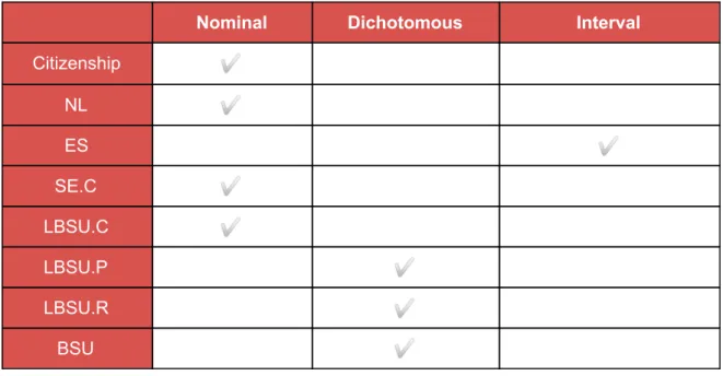
Table 3 illustrates features, with their types, which we have left after cleaning and transforming the raw data.
Nominal Dichotomous Interval
Citizenship ✅ NL ✅ ES ✅ SE.C ✅ LBSU.C ✅ LBSU.P ✅ LBSU.R ✅ BSU ✅ 18
MU ✅ JP1 ✅ MS ✅ MS.P ✅ LBSU.GPA ✅ H.GPA ✅ AS ✅ AR ✅ 19
4. Analysis/Results
4.1. Analysis of the existing model
The research question is to what extent admission score is correlated with student’s actual academic performance in Software Engineering programme at the University of Tartu. To answer this question let's first discuss current admission model. AS (admission score) is calculated using MS(motivation letter score) and LBSU.GPA (last bachelor degree GPA). We need to find how AS correlates with H.GPA (grade in UT). As we discussed in the previous section, AS, H.GPA, LBSU.GPA and MS are continuous and interval variables.
Correlation analysis measures the strength of association between two variables and the direction of the relationship [10]. In terms of the strength of relationship, the value of the correlation coefficient varies between +1 and -1. A value of ± 1 indicates a perfect degree of association between the two variables. As the correlation coefficient value goes towards 0, the relationship between the two variables will be weaker. The direction of the relationship is indicated by the sign of the coefficient; a + sign indicates a positive relationship and a – sign indicates a negative relationship [10]. The popular methods used in correlation analysis are Pearson and Spearman coefficient tests. The Pearson correlation coefficient is the most widely used. It measures the strength of the linear relationship between normally distributed variables. If the variables are not normally distributed or the relationship between the variables is not linear, than Spearman correlation method is more appropriate [11]. In order to choose suitable correlation method we checked if H.GPA and AS are normally distributed. We used Shapiro-Wilk normality test’s implementation in R programming language. The Shapiro–Wilk test is a test of normality in frequentist statistics. Here are the results for both AS and H.GPA respectively:
The null-hypothesis of this test is that the population is normally distributed. If the p value is less than the chosen alpha level, then the null hypothesis is rejected and there is evidence that the data tested are not normally distributed[12]. In R implementation, by default, alpha level is 0.05. As we can see from the output, for both variables the p-value > 0.05 implying that the distribution of the data are not significantly different from normal distribution. In other words, we can assume the normality of both variables.
To clarify, we illustrate the variables MS and H.GPA with normal q-q plots in Figure 3:
For AS, values vary from 75 to 95 and the deviations from the straight line are minimal. This indicates normal distribution.
The same pattern can be seen for GPA variable, where the values vary from 1.5 to 5.0 and points in the QQ-normal plot shows a straight diagonal line.
After checking that H.GPA and AS are normally distributed interval variables, we can safely Pearson’s method to find relationship between them. For that, we used cor.test function in R programming language:
In the result above :
● t is the t-test statistic value (t = 1.98), ● df is the degrees of freedom (df= 70),
● p-value is the significance level of the t-test (p-value = 0.05).
● conf.int is the confidence interval of the correlation coefficient at 95% (conf.int = [-0.001, 0.43]);
● sample estimates is the correlation coefficient (Cor.coeff = 0.23)[13]. We can interpret the result as the following: AS and GPA are not significantly correlated with a correlation coefficient of 0.23 and p-value of 0.05. For better understanding we can illustrate the results:
As we see from Figure 4, the relationship between the variables is almost unseen. That being said, we can answer to the first research question and claim that admission score calculation which is solely based on Bachelor’s GPA and motivation letter score is not meaningful enough and there is a room for improvements.
We also checked the correlation between MS and H.GPA and LBSU.GPA and H.GPA.
In Figure 5:
● The distribution of each variable is shown on the diagonal.
● On the bottom of the diagonal : the bivariate scatter plots with a fitted line
are displayed
● On the top of the diagonal : the value of the correlation plus the
significance level as stars. Each significance level is associated with a symbol : p-values(0, 0.001, 0.01, 0.05, 0.1, 1) <=> symbols(“***”, “**”, “*”, “.”, " “)
As we can see, LBSU.GPA and H.GPA are not correlated, the value of correlation is -0.02, on the other hand, the p-value is 0.8, which means that the result is not reliable. We got slightly better results for MS and H.G where the value of correlation is 0.34 and the result is more reliable with p-value of 0.003.
The final admission score of the applicant is calculated as a weighted sum of motivation letter score and normalized GPA with weights 2 and 3. According to our investigation, we would have better results if we put more weight to motivation score.
4.2. Feature selection
As a next step, we use machine learning techniques to identify the important features which affect the final grade of the student (H.GPA). We consider other parameters like experience, Master’s degree, University rankings and so on.
As we discussed in the previous chapter, we can use correlation analysis to measure association strength between two variables. In this chapter we will use correlation analysis to find out association strengths between other variables and H.GPA, where H.GPA is an interval (numeric) variable. However, correlation coefficient can not be calculated between two variables if one or both of them are nominal, since nominal variables cannot be compared to each other and thus we cannot have a positive or negative correlation. In our data, country-related fields are nominal and we will discuss them in given context later in this chapter.
For the rest of the data we can calculate pearson correlation coefficient. Since checking correlations between each pair of the variables could also give some interesting insights, we have calculated a correlation matrix for all the features (except nominal features, as mentioned above).
In Figure 6, the correlation between the features is shown with the colour and the size of the little squares. The bigger and darker the circle is, the stronger is the correlation. Blue colour shows positive correlation and orange is for the negative. Numbers inside squares correspond to p-values. Informally speaking, lower p-value means more reliability of corresponding correlation coefficient.
With this matrix we have identified several interesting patterns. MS and LBSU.GPA we have already discussed in the previous chapter. MS.P, which stands for plagiarism test results, showed negative correlation with H.GPA with quite high reliability (p-value of 0.03). It probably means that if applicant has plagiarized motivation letter, his/her motivation to study in host university is not high, hence the performance will be lower. This is a very interesting discovery that University was not paying enough attention to. (We hope this thesis won’t show high scores in plagiarism test)
Matrix also showed that age range and english scores are also negatively correlated with H.GPA. Those two results we will leave as facts, without possible further explanations.
In Figure 7, we have marked all the boxes corresponding to feature pairs that either did not have enough correlation coefficient, or did have it but with low reliability (high p-value). Under the diagonal, we have printed corresponding correlation coefficient in each box. With respect to H.GPA, we have the following features left as important ones: MS, MS.P, ES and AR.
Now let’s discuss nominal features. As we have mentioned, we cannot calculate correlation coefficients for those. We need to find the association patterns between nominal features and H.GPA. To achieve it, we have decided to use a feature selection algorithm named Boruta. The Boruta algorithm is a wrapper built around the random forest algorithm.
Random forest works by building several decision trees and making them operate as an ensemble. The key idea behind this is that even though individual decision trees are not good predictors, if their predictions have low correlations with each other, making them work together will give much better results.
Boruta algorithm tries to capture all the important, interesting features we might have in the admission dataset, with respect to H.GPA. It works by first shuffling data in all the columns one by one. Then it trains a random forest on shuffled data and checks the feature importance with Mean Decrease Accuracy [16]. Then it compares calculated feature importance with feature importance of the same feature from the
original data and if importance from real data is higher, It records a so-called ‘hit’. After a fixed number of iterations, the algorithm terminates. Then, based on a number of hits, it confirms or rejects the feature (that is, declares the feature as important or not important).
We have performed feature importance check with Boruta. The results are present in Table 4:
meanImp minImp maxImp normHits decision
MS 7.9911 4.2869 11.0682 0.9393 Confirmed MS.P 5.6069 2.3237 8.79903 0.8081 Confirmed LBSU.GPA 0.6161 -1.7614 2.3283 0.0101 Rejected AS 1.2451 -1.4831 2.9296 0.0101 Rejected Citizenship 7.6158 5.485 11.3 0.9495 Confirmed NL 3.1451 -1.7965 5.5556 0.5253 Tentative ES 0.2732 -1.1696 2.3731 0.0101 Rejected SE.C -0.4103 -2.4727 3.0139 0 Rejected LBSU.C 12.8029 8.3143 15.6086 0.9899 Confirmed LBSU.R 1.2819 -1.0584 3.4394 0.0404 Rejected LBSU.P 1.2435 -0.4778 3.3409 0.0303 Rejected JP1 -0.7653 -2.4294 1.0024 0 Rejected JS1 -0.5179 -1.6228 0.5937 0 Rejected AR -1.1805 -1.9147 0.041 0 Rejected MU -0.9258 -2.7711 1.8234 0 Rejected BSU 2.7793 0.9399 4.4574 0.4646 Tentative
As the algorithm runs for several iterations, we get several important values for features with shuffled data. Here, meanImp stands for the mean value of the feature
importance, maxImp for maximum, minImp for minimum and normHits is a normalised value of hits. Figure 8 is an illustration of a given table.
The plot shows the relative importance of each feature. The x-axis represents features, while the y-axis represents the importance. Green colour indicates the confirmation of the feature as important. Red indicates rejection and yellow indicates tentative confirmations, which means that the algorithm could not decide whether or not the feature is important because it was on the border of both.
As we can see several features are confirmed as important. According to Boruta algorithm, important features are LBSU.C, MS, Citizenship and MS.P.
However, before making any conclusions, let's take a look at Figure 9, which shows the distribution of LBSU.C.
Most of the applicants are from Azerbaijan, Ukraine, Nigeria, Pakistan, Turkey, Georgia, India and Russia. However, for a lot of the countries, we only have one or two applications. For those countries we can hardly say that citizenship correlates with H.GPA, due to the lack of data. For the rest of the countries, we can assume that there is a strong association between LBSU.C and H.GPA. To get a better understanding of LBSU.C’s importance, let’s take a look at the chart below:
As we can see from Figure 10, some countries, for example, Turkey, has worse grades in the last Bachelor, then at the University of Tartu (LBSU.G < H.G). For some, for example, Azerbaijan, the situation is vice-versa (LBSU.G > H.G). This tells us that based on LBSU.C we might normalize LBSU.G differently. For example, if we have two candidates, one from Azerbaijan and one from Turkey with the same LBSU.G’s, according to our dataset we should probably give higher admission score to the student from Turkey. On a higher level, this confirms our previous results that LBSU.C carries valuable information and should be considered when predicting student’s performance.
4.3. Academic performance prediction model
In this chapter, we produce models which predict the final grade of the students at the end of their studies. The final grade is number in the range of 1 to 5 (H.GPA). For better visualisation and understanding we have decided to bin H.GPA. We have mapped values from H.GPA to 4 intervals: from 1 till 2, from 2 till 3, from 3 till 4 and from 4 till 5. We stored them in a new variable, H.G (host university grade). In other words, using the binning method we transformed continuous variable H.GPA into categorical variable H.G with 4 categories: 2, 3, 4 and 5. We used H.G as a target value for the models. Since we have a categorical target variable, we build classification models.
After defining the nature of the problem, we selected predictor variables that models would use. In the previous chapter, we used correlation matrix and feature selection algorithm Boruta to choose some useful features from the admission dataset. Correlation matrix, that was calculated according to Pearson's correlation coefficient, showed that MS, MS.P, AR and ES are important features for predicting H.GPA, and correspondingly it’s binned version, H.G. However, it showed that MS and MS.P have higher correlation and p-values then AR and ES. Boruta algorithm showed that LBSU.C, MS, Citizenship and MS.P are important features. Thus, MS and MS.P’s importance was confirmed by both algorithms and we will definitely include them in our performance prediction model. AR and ES were rejected by Boruta algorithm. Citizenship and LBSU.C have nominal values and thus were not included in the correlation matrix. In our dataset, in most of the cases, Citizenship and LBSU.C values are identical. Thus, keeping both features would not add much valuable information. Thus, we have decided to keep one that showed higher importance according to Boruta algorithm. That is LBSU.C.
Thus, features that we have detected to be important and will use as predictor variables are MS, MS.P, AR, ES and LBSU.C.
In general, to test the model’s performance, the existing data are usually split into three parts: train, test and validation datasets. The model gets trained by train
dataset. Then, if the model has some parameters that can get tweaked, they get tweaked while checking the model’s performance on validation data. After tweaking the parameters, the actual performance is measured by running it on the test dataset. Since our dataset is very small we will not be using validation dataset, and we’ll split our data into two parts: train and test datasets. We chose ratio 7:3.
Below we discuss popular classification algorithms in educational data mining. Then we create three different models for each algorithm: One according to features that are used in the current model used in the University of Tartu, one with all the features that we extracted and one with features that we selected according to the feature importance analysis done in previous chapters. Afterwards, we compare classification algorithms and their performances on those three feature sets.
4.3.1. Selecting classification algorithms
It is important to choose the data mining method wisely. We have searched for related studies and found which algorithms work best with the kind of data that we have in educational data mining.
Below we will discuss Naive Bayes and Random Forest algorithms.
The results of the classification are measured with the following parameters:
● accuracy - the percentage of correctly classified instances out of all instances. ● Kappa - like classification accuracy. It is a degree of agreement of
effectiveness and reliability of the model. Kappa result can be interpreted as follows: values ≤ 0 as indicating no agreement, 0.01–0.20 as none to slight, 0.21–0.40 as fair, 0.41– 0.60 as moderate, 0.61–0.80 as substantial, and 0.81–1.00 as almost perfect agreement[20].
● p-value - the probability that the null hypothesis (hypothesis which the researcher tries to reject or nullify ) is true for the classification algorithm. The lower p-value means higher reliability of predictor.
● no information rate - error rate when the input and output are independent. accuracy should be higher than no information rate in order to say that the model is significant.
4.3.2. Naive Bayes
A Naive Bayes (NB) is a probabilistic machine learning algorithm used for classification tasks. It is based on Bayesian theorem. Bayesian theorem describes the probability of an event, based on prior knowledge of conditions that might be related to the event [18].
Bayes Theorem:
For two events, A and B, Bayes’ theorem allows to find out P(A|B) (the probability that event A happened, given that event B was positive) from P(B|A) (the probability that B happened, given that event A happened)[19]. Naive Bayes is called 'naive' because it makes the assumption that features of measurement are independent of each other. This is “naive” as this assumption is (almost) never true.
We preferred to use Naive Bayes to train our student performance prediction model because:
● It needs less training data compared to other classification methods. In our case, it is important because our dataset is small.
● It can handle both continuous and discrete data. ● Can be used for multi-class classification problems
We have trained the model with features that are used in current student performance prediction model using NB (Later referred to as NB_1). In the case of the current model, MS and LBSU.GPA are predictor variables and H.G is a target value. We used R packages ‘caret’ and 'e1071' which provides the Naive Bayes algorithm implementation. After the model was trained, we run it on our test dataset and got the following results:
Here, the accuracy of 0.26 means that only 26 percent of the test data were correctly classified, which is not a good result. Kappa is negative and the p-value is very high (93%), which indicates that the model is not effective and reliable. No information rate value also confirms that the model is not significant (0.39 > 0.26). In other words, predicting HG based on MS and LBSU.GPA using NB classifier is not accurate and reliable. For better illustration we can take a look at the so-called confusion matrix:
In confusion matrix, expected results for target value are shown down the side and predicted values are shown across the top. As we can see the number of incorrect predictions for each class: 2, 3, 4 and 5 are high.
Next, we trained student performance prediction model with all the features in our dataset (Later referred to as NB_2) and got better results:
Accuracy is still not high (34%), but it is higher than in the previous model. Kappa is low but positive, meaning that this model is more reliable. Same can be seen looking at p-value and no information rate which shows slightly better effectiveness and reliability compared to the model with currently used features.
From the confusion matrix, we can see that the predictions are still not accurate but improvements are noticeable. For example, we have fewer errors predicting class 5 and 4. However, the model was not able to predict class 2 and 3 well.
For our next model, we used the features which were selected according to feature importance analysis (Later referred to as NB_3). So, here the predictor variables are MS, MS.P, AR, ES and LBSU.C. This prediction model outperformed both models discussed above.
Accuracy is far away from being perfect, but it is almost two times better than the accuracy of NB_1. The value of Kappa is fair enough to agree that the model is reliable. No information rate is lower than accuracy and p-value is also low, which also implies that the model is more reliable and effective. The confusion matrix still shows a lot of mispredictions, but it is slightly better for classes 2, 5 and 4 compared to previous models.
Table 5 summarizes the results of all 3 models.
Accuracy P-Value Kappa
NB_1 0.26 0.9 -0.1
NB_2 0.34 0.7 0.1
NB_3 0.43 0.4 0.2
4.3.3. Random forest
Decision tree builds classification or regression models in the form of a tree structure. Random forest (RF) is a machine learning method for classification, regression and other tasks which operates by constructing a multitude of decision trees at training time. It is outputting the class that is the mode of the classes (classification) or mean prediction of the individual decision trees.
Random forest is widely used in Education Data Mining and, according to studies [1] and [5], it outperforms other classification algorithms in the same research field. Other than that:
● RF Can easily handle categorical features. ● It requires less preparation of the input data.
● Random forest applies the technique of bagging (bootstrapping) to decision tree learners. Bootstrapping enables the Random Forest to work well on relatively small datasets [21].
Like in the case of NB, we trained 3 models using RF classifier: the model with features that are currently used (Later referred as RF_1), the model with all the features (Later referred as RF_2) and the model with important features only (Later referred as RF_3).
In the following calculations, R packages called caret and randomForest are used. Below, we have results for RF_1:
We got the accuracy of just 21% which is a lower result then NB model trained with the same feature set (NB_1, 26% accuracy). Here, Like NB_1, Kappa is negative and the p-value is almost 100%, indicating that the model is not effective and reliable at all. No information rate value also confirms that (0.39 > 0.21). In other words, predicting H.G based on MS and LBSU.GPA using RF classifier is even less accurate and reliable compared to NB_1. The same can be seen by looking at the confusion matrix where false positives and false negatives are introduced in every class:
Below are the results for RF_2:
Like NB_2, this model also showed improvements in both accuracy and reliability criteria compared to RF_1. However, RF_2 outperformed NB_2 by showing better
accuracy of 43% compared to 34% accuracy of the model trained with NB_2. Here, Kappa is also low but positive, meaning that this model is more reliable. P-value and no information rate value also indicates slightly better effectiveness and reliability compared to NB_1.
In the confusion matrix, we can see the predictions with more true positives and true negatives compared to results of RF_1. We have fewer errors predicting class 5, and class 4. The model showed better results for class 3 compared to NB_2.
Next, used the only important features for training the model. Unfortunately, it didn’t show many improvements compared to the previous model (RF_2)
Here, Kappa is a little bit higher, which shows that the model might be more reliable than the previous one. Other than that, there is no difference between this model and the previous model. The same can be seen looking at the confusion matrix which is almost identical to the previous matrix.
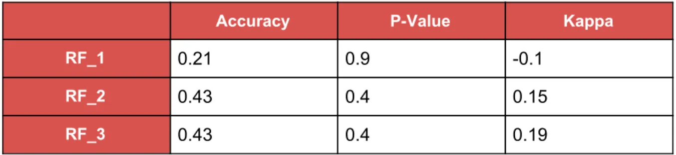
Table 6 summarizes RF classifier results trained against 3 datasets:
Accuracy P-Value Kappa
RF_1 0.21 0.9 -0.1
RF_2 0.43 0.4 0.15
RF_3 0.43 0.4 0.19
To sum up, both RF and NB showed that models with currently used features are not effective and accurate for predicting student academic performance. Both algorithms showed almost the same results. The main difference was that for NB, excluding the features which were not important show a noticeable difference. RF was able to achieve the same results with all the features.
In this chapter we showed that with features we detected as important ones, it is possible to improve the model efficiency almost twice, considering both accuracy and reliability.
5.
Conclusion
In this study, we focused on improving the admission process at the University of Tartu. To improve the process we identified the sources of the admission data and automated the process of admission application extraction by inventing a new software tool called DreamApplyParser. After that, we collected the data for the past 5 years using DreamApplyParser. After collecting the data we used the Input-Process-Output approach to analyze a current model of admission process and suggest a better one. In this process we explored, cleaned up and transformed the (anonymized) admission dataset.
We found out the relationship between admission score and student’s actual performance using correlation analysis. We performed Pearson correlation coefficient test between admission score and host university GPA. The results suggest that there is a positive correlation between those variables, but very weak, which means that higher admission score is weakly linked to higher GPA. However, there is a better correlation index for motivation letter score and GPA. According to our research results, we couldn’t see any correlation between LBSU.GPA (GPA of last bachelor’s degree) and host university GPA.
The main achievement of the study is identifying features which can help to improve the prediction of student’s academic performance. These features are:
● Motivation score (positively correlated with H.GPA)
● Plagiarism score of the motivation letter (negatively correlated with H.GPA) ● The country where the student got his/her last Bachelor’s degree
● English score (negatively correlated with H.GPA) ● Age (negatively correlated with H.GPA)
To get those results, we used the correlation matrix of Pearson correlation coefficients and Boruta algorithm.
To check the performance and accuracy of existing and new models we used classification algorithms: Naive Bayes and Random Forest. According to results, the new model outperformed the models with existing features almost twice, considering both accuracy and reliability.
5.1. Future improvements
The data which are used in Educational Data Mining is usually huge in size which gives an ability to achieve reliable results. In this research, it was not possible to collect a large amount of data for various reasons. The main reason was that the part of the data were still extracted manually like GPA which was time-consuming. The improvement of this study would be to automate the extraction of GPA from diploma images. Besides, it would be nice if the raw data contained more information about the applicant, for example, the GPA of all the universities the applicant has studied before which would help us to define better admission model.
6. Bibliography
[1] Maryam Zaffar, Manzoor Ahmed Hashmani and K. S. Savita, “Performance analysis
of feature selection algorithm for educational data mining”, 2018.
[2] Bo Guo, Rui Zhang, Guang Xu, Chuangming Shi and Li Yang, “Predicting Students
Performance in Educational Data Mining”, 2016.
[3] M. Nasiri, B. Minaei and Fereydoon Vafaei, “Predicting GPA and academic dismissal
in LMS using educational data mining: A case mining”, 2012.
[4] Jonnelle Marte, “Here’s how much your high school grades predict your future
salary”, 2014
[5] Anoop kumar M and A. M. J. Md. Zubair Rahman, “A Review on Data Mining
techniques and factors used in Educational Data Mining to predict student amelioration”,
2016.
[6] Azwa Abdul Aziz, Nor Hafieza Ismail, Fadhilah Ahmad, "First Semester Computer
Science Students' Academic Performances Analysis by Using Data Mining Classification
Algorithms", 2014.
[8] Nguyen Thai Nghe, Paul Janecek, and Peter Haddawy: A comparative analysis of
techniques for predicting academic performance; Asian Institute of Technology (AIT),
2007.
[9] Chen, P. Y., & Popovich, “Correlation: Parametric and nonparametric measures”.
Thousand Oaks, CA: Sage Publications, 2002.
[10] Statistics solutions, “Correlation (Pearson, Kendall, Spearman)”, 2019.
[11]Jan Hauke and Tomasz Kossowski, “COMPARISON OF VALUES OF PEARSON’S
AND SPEARMAN’S CORRELATION COEFFICIENTS ON THE SAME SETS OF
DATA”, 2011.
[12]THE SHAPIRO-WILK AND RELATED TESTS FOR NORMALITY, 2015
[13] Jacob Benesty, Jingdong Chen, Yiteng Huang and Israel Cohen, “Pearson
Correlation Coefficient”, 2009.
[14] Douglas G. Bonett and Thomas A. Wright, “Sample size requirements for estimating Pearson, Kendall and Spearman correlations”, 2000.
[15] Douglas M. Hawkins, “The Problem of Overfitting”, 2004.
[16] Hong Han ; Xiaoling Guo and Hua Yu, “Variable selection using Mean Decrease
Accuracy and Mean Decrease Gini based on Random Forest”, 2016.
[17] Dr. Saurabh Pal, “Mining Educational Data Using Classification to Decrease the
Dropout Rate of Students ”, Department of Computer Applications, VBS Purvanchal
University, Jaunpur – 222001 (U.P.), India, 2012.
[18] Tina R. Patil and Mrs. S. S. Sherekar Sant Gadgebaba Amravati University,
Amravati, “Performance Analysis of Naive Bayes and J48 Classification Algorithm for
Data Classification”, 2013.
[19]Statistics How To, “Bayes’ Theorem Problems”, 2014.
[20] Biochem Med (Zagreb), Interrater reliability: the kappa statistic, 2012.
Non-exclusive licence to reproduce thesis and make thesis public I, Ketevan Toria
1. herewith grant the University of Tartu a free permit (non-exclusive licence) to
reproduce, for the purpose of preservation, including for adding to the DSpace digital archives until the expiry of the term of copyright,
of my thesis
Predicting Academic Performance From Admission Scores and Application Data – A Case Study,
supervised by Marlon Dumas and Irene-Angelica Chounta
2. I grant the University of Tartu a permit to make the work specified in p. 1 available to the public via the web environment of the University of Tartu, including via the DSpace digital archives, under the Creative Commons
licence CC BY NC ND 3.0, which allows, by giving appropriate credit to the
author, to reproduce, distribute the work and communicate it to the public, and prohibits the creation of derivative works and any commercial use of the work until the expiry of the term of copyright.
3. I am aware of the fact that the author retains the rights specified in p. 1 and 2.
4. I certify that granting the non-exclusive licence does not infringe other
persons’ intellectual property rights or rights arising from the personal data protection legislation.
Toria Ketevan
14/08/2019