DEVELOPMENT, IMPLEMENTATION AND EVALUATION OF NARROW LINEWIDTH EXTERNAL CAVITY DIODE LASERS FOR USE IN RAMAN GENERATION EXPERIMENTS

(1)

DEVELOPMENT, IMPLEMENTATION AND EVALUATION OF NARROW LINEWIDTH EXTERNAL CAVITY DIODE LASERS FOR USE IN RAMAN GENERATION

EXPERIMENTS

By

JOSHUA W. HENRY

A THESIS SUBMITTED IN PARTIAL FULFILLMENT OF THE REQUIREMENTS FOR THE DEGREE OF

(2)

ACKNOWLEDGMENTS J.T. Green, N. Proite and D.D. Yavuz

(3)

TABLE OF CONTENTS page ACKNOWLEDGMENTS. . . 2 LIST OF TABLES . . . 5 LIST OF FIGURES . . . 6 ABSTRACT . . . 8 CHAPTER 1 Experiment Overview . . . 9

1.1 Scope and Motivation . . . 9

1.1.1 Synopsis and End State . . . 9

1.1.2 Stokes and Anti-Stokes Radiation . . . 9

1.1.3 The Experiment In Practice and Operation . . . 10

1.1.4 CW Raman Generation and Past Achievements . . . 12

1.2 Narrow Linewidth Lasers . . . 13

1.2.1 Laser Linewidths . . . 13

1.2.2 Methods of Measuring Laser Linewidth . . . 15

1.2.3 Role in Stokes Generation Experiments . . . 19

2 Diode Lasers . . . 22

3 ECDL Configurations And Performance . . . 24

3.1 Free Running Diode Spectra . . . 25

3.2 Littrow Configured ECDL and Integration With Erbium Doped Fiber Amplifier (Figure 3-3, Table 3-1) . . . 25

3.2.1 The Grating Equation . . . 26

3.3 Initial IFS-ECDL Configuration (Figure 3-6, Table 3-2) . . . 29

3.4 Modified IFS-ECDL With HT-IF. (Figure 3-7, Figure 3-8, Table 3-3) . . . 32

3.5 Modified IFS-ECDL With MT-IF (Figure 3-9, Figure 3-10, Table 3-4) . . . 34

3.6 IFS-ECDL With HT-IF and Low Reflectivity OC (Figure 3-11, Figure 3-12, Table 3-5) . . . 37

3.7 IFS-ECDL With Dual Narrowband Interference Filters. (Figure 3-13, Figure 3-14, Figure 3-15, Table 3-6) . . . 40

3.8 IFS-ECDL With HT-IF and Broad Spectrum (Figure 3-1) Diode . . . 41

3.9 IFS-ECDL With HT-IF and Variable Reflectivity At OC (Figure 3-16, Figure 3-17, Table 3-8) . . . 42

4 Conclusion . . . 49 APPENDIX

(4)

A.1 Basic Development . . . 50

A.2 Eigenmodes . . . 53

B Gaussian Mode Matching Of Incident Beam To Cavity Waist Using Mode Matching Optics . . . 56

C A Start To Finish MATLAB Code For Streamlined Importation, Analysis And Fitting Of Post-Cavity Spike Oscilloscope Data . . . 60

C.1 Oscopedata.m Main Function. . . 60

C.2 SampleFit.m Curve Fitting Function . . . 65

(5)

LIST OF TABLES

Table page

1-1 Power Characteristics Of IPG Photonics Fiber Amplifier . . . 16

3-1 Characterization Of Standard Grating Stabilized-ECDL (Figure 3-3) . . . 29

3-2 Characterization Of Initial IFS-ECDL With HT-IF (Figure 3-6) . . . 32

3-3 Characterization Of IFS-ECDL With HT-IF (Figure 3-7, Figure 3-8) . . . 35

3-4 Characterization Of IFS-ECDL With MT-IF (Figure 3-9, Figure 3-10) . . . 36

3-5 Characterization Of IFS-ECDL With HT-IF And 10% OC (Figure 3-11, Figure 3-12) . 39 3-6 Characterization Of IFS-ECDL With Dual Interference Filters And 30% OC (Figure 3-13, Figure 3-14, Figure 3-15) . . . 40

3-7 Characterization Of IFS-ECDL With Eagleyard Diode And HT-IF . . . 43

3-8 Characterization Of IFS-ECDL With HT-IF And Moderate Variable Reflectivity OC . . 45 3-9 Characterization Of IFS-ECDL With HT-IF And Very High Variable Reflectivity OC . 45

(6)

LIST OF FIGURES

Figure page

1-1 Vibrational Stokes Radiation: Energy Of Emitted Radiation Is Less Than That Of

Incident Photon Energy . . . 10

1-2 Experimental Setup Generating 300 mW CW Stokes Radiation . . . 11

1-3 Legend Of Common Optical Modules . . . 12

1-4 High Finesse Cavity Exploded View. Design: J.T. Green . . . 16

1-5 Integrating The Laser To Be Characterized With Amplification And High Finesse Cavity Elements. Figure 1-3 Applies To This Schematic . . . 17

1-6 Spatial Properties Of Beam Before Fiber Amplifier . . . 18

1-7 Spatial Properties Of Beam After Fiber Amplifier . . . 20

3-1 Eagleyard Unstabilized Laser Diode Spectrum . . . 26

3-2 QPhotonics Unstabilized Laser Diode Spectrum . . . 27

3-3 Custom Fabricated, Temperature Controlled Grating Tuned ECDL (Table 3-1) . . . 27

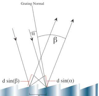
3-4 Geometry Of Diffraction: For planar wavefronts, two parallel, in phase rays are incident upon the grating and spaced one groove apart by a distance d. In order to observe constructive interference upon diffraction, the valued(sin(α) + sin(β))must be an integral number of path lengths. . . 28

3-5 Angle Of Rotation For Narrowband Interference Filters . . . 31

3-6 IFS-ECDL With Intra-Cavity Cat’s Eye And HT-IF (Table 3-2) . . . 33

3-7 IFS-ECDL With Aspherical Lens Focus At OC And HT-IF (Figure 3-8, Table 3-3) . . 34

3-8 Peak And Gaussian Fit: IFS-ECDL With Aspherical Lens Focus At OC And HT-IF (Figure 3-7, Table 3-3) . . . 35

3-9 IFS-ECDL With Aspherical Lens Focus At OC And MT-IF (Figure 3-10, Table 3-4) . . 36

3-10 Optical Spectrum: IFS-ECDL With Aspherical Lens Focus At OC And MT-IF (Figure 3-9, Table 3-4). . . 37

3-11 IFS-ECDL With Aspherical Lens Focus At 10% OC And HT-IF (Figure 3-12, Table 3-5) . . . 38

3-12 Peak And Gaussian Fit: IFS-ECDL With Aspherical Lens Focus At 10% OC And HT-IF (Figure 3-11, Table 3-5) . . . 39

(7)

3-14 Peak And Gaussian Fit: IFS-ECDL With Dual Narrowband Interference Filters (Figure

3-13, Figure 3-15, Table 3-6) . . . 42

3-15 Optical Spectrum: IFS-ECDL With Dual Narrowband Interference Filters (Figure 3-13, Figure 3-14, Table 3-6) . . . 43

3-16 IFS-ECDL With HT-IF And Variable Reflectivity OC (Figure 3-17, Figure 3-18, Figure 3-19, Table 3-8, Table 3-9) . . . 44

3-17 Multiple Superposed Peaks And A Single Gaussian Fit: IFS-ECDL With HT-IF And Variable Reflectivity (Figure 3-16, Table 3-8) . . . 46

3-18 Power Output As A Function Of OC Reflectivity . . . 47

3-19 Mean Linewidth As A Function Of OC Reflectivity . . . 48

A-1 Propagation Of Incident Beam Through A Fabry-Perot Resonator . . . 50

A-2 The Free Spectral Range Of A Fabry-Perot Resonator . . . 52

A-3 A Finite Volume Of Cavity Resonances . . . 53

B-1 Overlapped Cavity And Beam Waists . . . 57

B-2 Section One Mathematica Code: ABCD Matrix Beam Propagation . . . 58

(8)

Abstract of Thesis Presented to the Graduate School of the University of Wisconsin in Partial Fulfillment of the

Requirements for the Degree of Master of Science

DEVELOPMENT, IMPLEMENTATION AND EVALUATION OF NARROW LINEWIDTH EXTERNAL CAVITY DIODE LASERS FOR USE IN RAMAN GENERATION

EXPERIMENTS By

Joshua W. Henry December 2009 Chair: Baha Balantekin

Major: Physics

Multiple configurations of external cavity diode lasers were designed, constructed and evaluated for tunability, stability, power output and spectral characteristics near the 1064 nm wavelength. A reliable design, incorporating a diffraction grating mounted in the Littrow configuration, delivering 32 mW of continuous wave (CW) power and exhibiting a full width at half maximum linewidth (FWHM) of 573.2 kHz served as the seed laser for coupling to a high power erbium doped fiber amplifier for experiments in both vibrational and rotational Raman generation in molecular deuterium (D2). Additionally, novel designs were constructed and evaluated utilizing an intra-cavity interference filter and partially reflecting out-coupler. The best performing configuration of the interference filter stabilized external cavity diode laser (IFS-ECDL) yielded an output power of 12.9 mW and a minimum consistently achieved FWHM linewidth of 317 kHz, measured by coupling to a cavity of high finesse (F = 22764).

(9)

CHAPTER 1

EXPERIMENT OVERVIEW

1.1 Scope and Motivation 1.1.1 Synopsis and End State

Stimulation of Raman scattering in a high finesse laser cavity containing low pressure deuterium gas is a first step in developing the technique of molecular modulation in the continuous wave light regime [4]. This Stimulated Raman Scattering (SRS), subject to certain pumping, pressure and temperature conditions, is equivalent to the interaction of two photons with the gas. The emitted spectra are in two bands equally separated from the initial frequency by the amount of energy transferred to or from the gas. At high pumping levels, higher order Raman spectra are observed when the Raman spectrum becomes self-regenerative. The resulting spectrum is a series of SRS peaks with decreasing amplitudes. In the absence of a seeding laser beam, the SRS spectrum is built up with spontaneous emission. As a mitigator of the intrinsic noise resulting from spontaneous processes, a seed laser beam can initiate the process. The process has been successful in the pulsed light regime where 200 Raman sidebands ranging in wavelength from 1.06µm to 195 nm were produced from a coherently prepared D2/H2gas [11].

Using pump beams of 1064 nm and 1550 nm in a laser cavity of high finesse for both pump beam and generated wavelengths, this experiment seeks to produce such broad bandwidth spectra in the continuous wave light regime.

1.1.2 Stokes and Anti-Stokes Radiation

Stokes radiation (its counterpart, anti-Stokes Radiation, is the converse of the subsequently described process) is essentially half of the process described above. It is the product of the interaction of a single photon of specific energy such that it transfers some energy to the object of its interaction (a molecule in a gas, an atom in a crystal lattice, etc.) in the form of either linear, rotational or electronic energy. It is, in a classical sense, the inelastic scattering of a photon with some object atom or molecule. In perturbation theory, the effect corresponds to the absorption

(10)

atom in a crystal lattice, bonding energy constrains this transfer of energy and momentum to linear or vibrational motion (a phonon), whereas in a molecular gas multiple types of energy transfer are allowed.

∆E_i=hν₀

γ

_→

∆E_e= -h(ν₀-νv)

∆E_v=hν_v

Figure 1-1. Vibrational Stokes Radiation: Energy Of Emitted Radiation Is Less Than That Of Incident Photon Energy

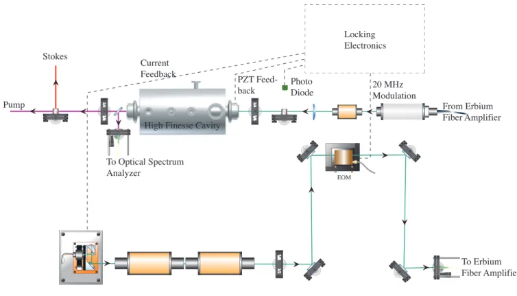
1.1.3 The Experiment In Practice and Operation

Figure1-2is a schematic of the original experiment conducted with a single 1550 nm pump laser beam. A legend in Fig.1-3is located on page12. When the experiment is expanded to include a second pump beam at 1064 nm, a similar system operating in parallel is required. At either wavelength, the laser source is a custom designed ECDL constructed by our group. The design shares heritage with one described in [1], with details and modifications described in detail in Sec. 3.2.

The beam traverses two Faraday isolators which act as optical diodes, followed by an electro-optic modulator (EOM) which superposes 20 MHz sidebands (phase modulation) on the laser spectrum. These sidebands serve two purposes. The primary purpose is to aid in locking the laser to the cavity post amplification. The secondary purpose, and more pertinent to the subject of this dissertation, is to give a clear demarcation of the relationship between frequency and time in

(11)

λ/ 2 λ/ 2 EOM To Erbium Fiber Amplifier From Erbium Fiber Amplifier Locking Electronics λ/ 4 λ/ 4 Photo Diode Current Feedback PZT Feed-back 20 MHz _Modulation λ/ 4 λ/ 4 To Optical Spectrum Analyzer

High Finesse Cavity Stokes

Pump

Figure 1-2. Experimental Setup Generating 300 mW CW Stokes Radiation

The beam is conditioned further via a beam cube and waveplate combination to control power and is finally propagated through a Glan-Taylor polarizer. The beam is coupled to an IPG Photonics erbium doped fiber amplifier via a single-mode fiber. Input power is constrained to the range of 5-10 mW and output power is scalable from 2 W to 30 W. The amplifier preserves both polarization and frequency characteristics of the input beam. Since this thesis distills to the evaluation of narrow linewidth laser spectra, any beam amplified must not be affected in the frequency spectrum by the amplifier. When specifically addressing the question of whether amplification adds appreciable noise photons, an amplification of 40 dBm adds approximately 104_{noise photons to the signal, which is negligible [7]. Thus, the frequency spectrum of an input} beam which exhibits a FWHM linewidth on the order of hundreds of kilohertz is unchanged by large amplifications.

Post amplifier, the beam is again isolated and via a mode matching lens (MML) coupled to a high finesse cavity with finesseF = 22764. A photodiode post cavity records output powers.

(12)

current) and low speed (diffraction grating piezo-electric transducer or PZT) electronic control of the ECDL. Control is achieved via the Pound-Drever-Hall method.

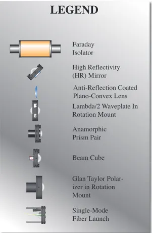
LEGEND

Faraday Isolator High Reflectivity (HR) Mirror Anti-Reflection Coated Plano-Convex Lens λ/ 2 λ/ 2 Lambda/2 Waveplate In Rotation Mount Anamorphic Prism Pair Beam Cube Glan Taylor Polar-izer in Rotation Mount

Single-Mode Fiber Launch

Figure 1-3. Legend Of Common Optical Modules

1.1.4 CW Raman Generation and Past Achievements

In order to achieve broad bandwidth Raman generation in a gas filled cavity, the molecules must be prepared in a maximally coherent state. The Raman spectrum can be collinearly

generated using two slightly detuned pump laser beams. In order to avoid pressure broadening effects, the gas pressure is maintained as low as possible while still maintaining an appreciable cross section of photon-D2molecule interaction within the cavity.

(13)

output power was generated [4]. Furthermore, since the generation occurred within a cavity of extremely high finesse, the output power was contained within an ultra narrow linewidth on the level of a few kilohertz.

1.2 Narrow Linewidth Lasers

The end-state of this project was the development of a narrow linewidth laser to act as second pump beam source which offered the following desirable traits:

• Linewidth on the order of tens of kilohertz

• Power output of at least 20 mW for coupling to fiber amplifier

• Center wavelength near 1064 nm

• Stable single-mode operation

• Single-mode tunability between 1055 nm and 1068 nm

These are ambitious stipulations. A narrow linewidth laser operating at 1064 nm with a linewidth of 15 kHz and fiber coupled output is readily available from JDS Uniphase

Corporation, however the laser is not tunable. The existing Littrow configured ECDL exhibits robust tunability, good power characteristics and wide-range wavelength tunability (single-mode operation is easily maintained between free spectral range transitions); however, its spectrum is an order of magnitude higher in the linewidth category. At the risk of divulging results prior to proper discussion of all factors in play, the more promising IFS-ECDL with variable output coupler reflectivity offered a promising trend toward narrow linewidths; unfortunately, power output was attenuated at such a rate that the beam was not sufficient to seed the fiber amplifier to obtain linewidth measurements at the tens of kilohertz level.

1.2.1 Laser Linewidths

An exploration of the nature of laser linewidths yields insight into the causes of and solutions to laser linewidth broadening. The Schawlow-Townes equation was calculated before the first laser was experimentally demonstrated. For a laser with a cavity bandwidth∆νc and

(14)

∆νlaser =

πhν(∆νc)2 Pout

(1–1) wherehis Planck’s constant. Fundamentally, the linewidth of a laser is proportional to the

square of the laser cavity bandwidth over its output power. However, due to experimental noise sources to include mechanical vibrations, temperature fluctuations and, specifically related to laser diodes, power source fluctuations, this linewidth is unachievable on a practical level. As demonstrated in AppendixA, the linewidth of a laser cavity can be reduced by extending its length. This occurs at the cost of a decreased free spectral range which, in turn, impedes conjunctive stable single-mode operation and tunability. Furthermore, a longer laser cavity is more difficult to mechanically stabilize.

The Schawlow-Townes equation is a representation of overall noise due to spontaneous emission in resonator modes of a free running laser cavity. Signal noise can be classified in two ways: phase noise, or fluctuation in the optical phase of a signal, and intensity noise, or the fluctuation in the optical intensity of a signal.

For simple systems, the linewidth of a laser can approach the Schawlow-Townes linewidth if experimental noise sources or technical factors are effectively mitigated. However, even in the case where a semiconductor laser (laser diode) was highly technically controlled, its linewidth was far in excess of the fundamental linewidth described by Schawlow-Townes.

In 1982, it was shown in a well developed and elegant treatment of the theory of semiconductor lasers by Charles H. Henry that there is a non-linear coupling of phase and intensity noise in the semi-conducting material [5]. The coupling is a result of the dependence of the refractive index on the carrier density in the semiconductor. While avoiding presentation of a facsimile of Henry’s work, it was shown that the power spectrum of a phase-intensity coupled system was Lorentzian in form with a FWHM of:

∆f = R

4πI(1 +α

(15)

whereRis the rate of average spontaneous emission andI is the average intensity. This equation is in its simplest theoretical form. Henry proceeded to show that an experimental extension from this point, which involves expressingI in terms of output power per facet and incorporating waveguide losses and standardexpgL_{gain within the cavity, gives a semiconductor laser}

linewidth which is broadened by the factor (1 +α2_{). In Henry’s derivation, he obtains a value} ofα = 5.4(αis unitless) for an AlGaAs semiconductor laser. This agreed with experimental data which fell within a range of4.6₋6.2and the theory is generally accepted as the source of semiconductor laser linewidth broadening. The experimental implication is that an unstabilized laser diode has a bandwidth of_∼100 MHz.

1.2.2 Methods of Measuring Laser Linewidth

There are multiple techniques for measuring laser linewidths. For lasers with large linewidths (e.g. Fig.3-1), a standard optical spectrum analysis can be performed. With single-frequency lasers, the self-heterodyne technique involves delaying a branch of the laser via a long, single-mode optical fiber and subsequent overlapping of the two signals. The resulting beat frequency is recorded and analyzed. A method akin to the self-heterodyne setup is the use of a laser of known operational characteristics with similar or lower noise attributes and the recording of a beat note between this laser and the laser to be characterized.

In a final method, which we use for its simplicity and practicality of implementation,1 _the frequency fluctuations of the laser can be converted to intensity fluctuations using a frequency discriminator (a high finesse cavity). Since the finesse of the cavity was much higher than that of our source laser cavity, de-convolution of the measured intensity fluctuations was not necessary.

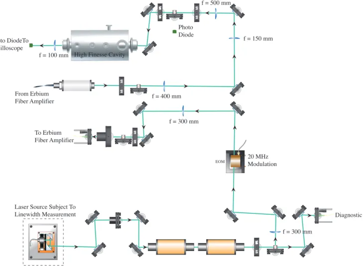
Figure1-5is a schematic of our laser linewidth measurement system. The beam is directed through an anamorphic prism pair which spatially compresses the wider axis of the cross-sectional profile of the beam in order to propagate a symmetric beam throughout the

(16)

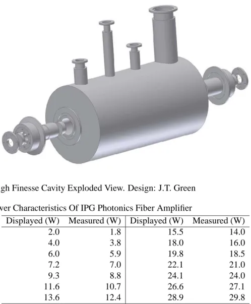
Figure 1-4. High Finesse Cavity Exploded View. Design: J.T. Green Table 1-1. Power Characteristics Of IPG Photonics Fiber Amplifier

Displayed (W) Measured (W) Displayed (W) Measured (W)

2.0 1.8 15.5 14.0 4.0 3.8 18.0 16.0 6.0 5.9 19.8 18.5 7.2 7.0 22.1 21.0 9.3 8.8 24.1 24.0 11.6 10.7 26.6 27.1 13.6 12.4 28.9 29.8

experiment. The beam proceeds through two Faraday isolators and is split at a beam cube for optical spectrum analysis2_{. An EOM superposes 20 MHz sidebands at the narrowest section} of the beam in a telescope. The beam is re-collimated and coupled to the fiber amplifier. The fiber amplifier did not display input power from the seed beam. For this reason, the delicate operation of coupling a laser beam to a single-mode fiber was difficult. Therefore, the beam was first coupled to a single-mode fiber then coupled to the fiber of the amplifier with a fiber

(17)

High Finesse Cavity From Erbium Fiber Amplifier 20 MHz Modulation EOM λ/ 2 λ/ 2 To Erbium Fiber Amplifier Diagnostic Photo Diode f = 400 mm f = 300 mm f = 150 mm f = 500 mm f = 100 mm Photo DiodeTo Oscilloscope

Laser Source Subject To Linewidth Measurement λ/ 2 λ/ 2 f = 300 mm λ/ 2 λ/ 2 λ/4 λ/4 λ/ 2 λ/ 2

Figure 1-5. Integrating The Laser To Be Characterized With Amplification And High Finesse Cavity Elements. Figure1-3Applies To This Schematic

coupler. Net power pre and post fiber coupler saw a reduction of about 10%. Minimum input power for the fiber amplifier is specified at 5 mW by the manufacturer; this was easily achieved if pre-fiber coupler power was 6 mW or better. Table1-1gives measured output powers of the fiber amplifier.

The output of the fiber amplifier immediately encountered a beam cube siphoning the majority of the power (minimum output was 2 W) into a beam dump. The remaining signal was conditioned with MML’s (see AppendixCfor details). Aλ/2- beam cube -λ/4series acted to 1) isolate the signal reflected from the front window of the cavity from the fiber amplifier and

(18)

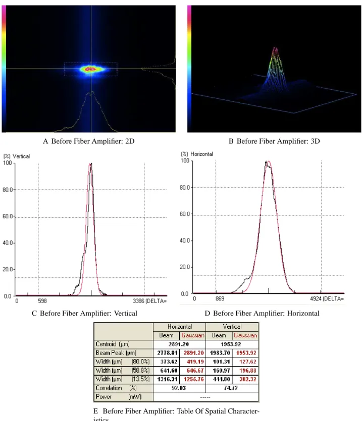
A Before Fiber Amplifier: 2D B Before Fiber Amplifier: 3D

C Before Fiber Amplifier: Vertical D Before Fiber Amplifier: Horizontal

E Before Fiber Amplifier: Table Of Spatial Character-istics

(19)

2) direct the reflected signal to a photodiode. The cavity transmitted signal was directed into a high-speed photodiode which was subsequently fed to an oscilloscope.

The cavity was designed for use with both 1064 nm and 1550 nm signals. It featured rigid construction with AR coated windows, AR front face and extremely high reflectivity (EHR) coated convex interior faces at both wavelengths. The cavity also featured an integrated hollow PZT at one end and overlapping liquid-nitrogen (N2) and vacuum chambers for thermodynamic optimization.3 The cavity had an overall length (interior mirror face to interior mirror face) of 0.27 m.

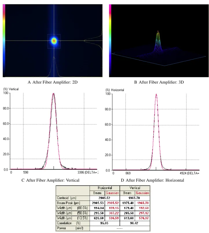
The spatial mode characteristics of the beam are of high importance in manipulation of atoms and for efficiency in fiber coupling. Therefore we examined the beam profile immediately before and after the fiber amplifier with a Newport CCD camera. The data in Fig. 1-6and Fig. 1-7are self-explanatory; though even our best pre-amplifier beam would be considered poor for delicate experiments. The fiber amplifier and single-mode fiber combination corrected much of the spatial aberration of the incident beam.

1.2.3 Role in Stokes Generation Experiments

The high finesse of the cavity allows only small portions of the frequency spectrum of a laser beam to achieve resonance in the Gaussian TEM00mode of the cavity. The electronics developed by our group, which condition the laser at the ECDL in such a fashion that the laser linewidth is reduced to match the cavity resonances, function well. However, even with active feedback, only approximately 30% of incident energy actually enters the cavity and participates in adiabatic preparation of the D2gas. A laser with a reliable linewidth below that of a standard grating tuned ECDL (on the order of .5 MHz) decreases the electronic conditioning requirements of the Pound-Drever-Hall method.

3_{This capacity was not necessary for linewidth measurements; it will be crucial for high}

(20)

A After Fiber Amplifier: 2D B After Fiber Amplifier: 3D

C After Fiber Amplifier: Vertical D After Fiber Amplifier: Horizontal

E After Fiber Amplifier: Table Of Spatial Characteris-tics

(21)

Therefore, in pursuit of an optimal seed laser for this experiment, different types of ECDL’s are developed, tested and compared against each other and the standard diffraction grating tuned configuration for their performance in power output, linewidth, tunability and stability. What follows revolves around this process and provides a blueprint for designing and constructing the novel configurations and an evaluation of the nature of diode lasers.

(22)

CHAPTER 2 DIODE LASERS

All lasers used in the experiment were based on laser diode packages designed to emit near a wavelength of 1064 nm. A broad definition of a laser diode is any semiconductor laser which exhibits gain when current is passed through a p-n or p-i-n structure.1 _{When the electrons and} holes in the structure recombine, their energy is released as a photon. In the absence of some optical feedback, the process is spontaneous.

The construction of our laser diodes is of the edge-emitting form. Emission wavelength is determined, roughly, by the bandgap of the semiconductor. The semiconductor material used in the experiment’s laser diodes was InGaAs or a phosphated composition InGaAsP.

In general, a laser diode of the edge-emitting/cleaved construction emits a highly divergent astigmatic output beam. The beam’s spectral characteristics exhibit an optical bandwidth of a few nanometers.2 This relatively large bandwidth is the result of multiple longitudinal resonator modes within the semiconductor cavity (a waveguide).

Laser diodes exhibit certain advantages over traditional laser pump sources. Additionally, laser pumping displays the following advantages over lamp pumping:

• Directional control of optical pump beam

• Good spectral overlap potential between pump beam and absorption band in gain medium

• Ability to match inversion profile created by pump beam to fundamental laser resonator mode in gain medium (mode matching)

Concerning the desirable qualities of laser diodes versus traditional laser pump sources:

1_{A p-i-n structure has an intrinsic (i) or undoped layer between the positive (p) and negative}

(n) regions which increases quantum efficiency and decreases capacitance [9].

2_{One laser diode used in this experiment is an exception to this statement. Its spectral}

(23)

• Diode modules exhibit long lifetimes. Mean time between failures (MTBF) for CW diodes is 5,000 to 20,000 hours3

• Laser diodes have a high innate electro-optical efficiency (ηD) of 50% or greater • Since the diode modules generate less heat, cooling requirements are reduced

• Weight and volume requirements are much less

• Modularity and interchangeability: Laser diode modules are obtained in standard packages and, within constraints of pin-outs and power requirements, are interchangeable within the existing mounting, temperature and current control system

The significant challenge with respect to the use of laser diodes is the aforementioned large spectral bandwidth of their free running output beam and how to effectively and reliably select a single mode of operation from the many modes extant in such a beam. Methods to achieve this are described in the remainder of this dissertation.

(24)

CHAPTER 3

ECDL CONFIGURATIONS AND PERFORMANCE

All ECDL configurations are comprised of a gain medium and an external optical feedback system. There are two categories of tunable ECDL configurations. The first relies on diffraction gratings as a combined wavelength selection and optical feedback component. The other category is relatively new and utilizes an intra-cavity narrowband interference filter for wavelength

selection and a separate partially reflective output coupling mirror for optical feedback. The amount of optical feedback is crucial in ECDL operation. Even very low levels of external feedback have been shown to affect laser diode operation [12]. Strong levels of feedback increase the probability of maintaining a low threshold current, continuous tuning and a narrow linewidth.

This thesis characterizes the diffraction grating tuned and stabilized ECDL primarily as a means of comparison for the IFS-ECDL configurations developed and tested. To our knowledge, of the IFS-ECDL configurations which follow, all but the first (Fig. 3.3) are novel in their design and operation at 1064 nm. Figure3.3is a design described in [2] and is novel in its operation at 1064 nm.

Before proceeding to the configurations themselves and associated results, the linewidths we report necessitate explanation. Our results are achieved by coupling the laser to a cavity of extremely high finesse and evaluating the transmitted signal with a high speed photodiode and oscilloscope. In this way, we can be confident that the signal we evaluate is the true laser linewidth and all reported linewidth values are the FWHM of the actual data sets; in order to ensure a low standard deviation at a high level of confidence we obtained 16 sample peaks per configuration. However, in [2] and [3], much lower linewidths are reported for similar signals. Both groups obtained their linewidth data via either self-heterodyne or comparison with a laser of known linewidth; they analyzed and interpreted their data using a different fitting algorithm. These groups fit the “tails” of their data with a Lorentzian function which narrowed reported

(25)

linewidth is, in fact Lorentzian in its form [10], and that the net peak is a combination of these Gaussian broadened Lorentzian peaks, is duly noted, we believe that the FWHM of the actual peak is the complete story of the laser and have therefore reported these values for linewidths. When fitting our data via the Lorentzian model we indeed obtained linewidths which were reduced by factors of ten to twenty times the values we report.

As a final note on the fitting process, a perusal of AppendixCdetails the methods used to properly fit the actual peak and calculate its FWHM.

3.1 Free Running Diode Spectra

As a precursor to elaboration on the design and characterization of these successful ECDL configurations, a short discussion of the free-running, unstabilized or “raw” spectra is also in order. As discussed in Sec. 2, different laser diode packages exhibit different unstabilized output spectra depending on their construction (edge or surface emitting) and anti-reflection coatings on their cleaved facets. In this experiment, two diode modules were tested, each emitting, to some degree or another, at or near 1064 nm.

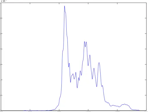
The first diode, manufactured by Eagleyard Photonics, was constructed with a high-reflectivity back face and anti-reflection coating on the output face. Its spectrum in Fig.3-1spanned nearly 150 nm.

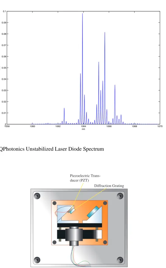
The second laser diode was manufactured by QPhotonics was also constructed with a

high-reflectivity back face and anti-reflection coating on the output face and possessed a spectrum (Fig. 3-2) which spanned only a few nanometers and exhibited the commonly appearing peaks of a Fabry-Perot cavity. This diode proved to be highly efficient when operating in conjunction with an interference filter and output coupling mirror for stabilization.

3.2 Littrow Configured ECDL and Integration With Erbium Doped Fiber Amplifier (Figure3-3, Table3-1)

The Littrow configured ECDL is a reliable design and has achieved a narrow linewidth (350 kHz) at a wavelength of 780 nm [1]. Our modified version of the ECDL described in [1]

(26)

850 900 950 1000 1050 1100 0 0.5 1 1.5 2 2.5 3 3.5x 10 −5 nm W

Figure 3-1. Eagleyard Unstabilized Laser Diode Spectrum

placed on a copper plate and thermally isolated from a massive aluminum base (acting as a heat sink) with plastic retainer screws. Thus, the only appreciable mode of energy transfer between the laser-plate assembly and heat sink base is a Peltier thermoelectric cooler (TEC) which is controlled by a Newport temperature controller. The controller receives its feedback from a 10K ohm thermistor situated adjacent to the collimating tube. The base is milled to accept a monolithic polycarbonate resin block which provides near-total draught exclusion.

3.2.1 The Grating Equation

The grating provides wavelength selection and optical feedback in the system. From Fig. 3-4, Eq. (3–1) can be geometrically derived:

(27)

10580 1060 1062 1064 1066 1068 1070 0.01 0.02 0.03 0.04 0.05 0.06 0.07 0.08 0.09 0.1 nm mW

Figure 3-2. QPhotonics Unstabilized Laser Diode Spectrum

Piezoelectric Trans-ducer (PZT)

(28)

Grating Normal d sin(β)

β

d sin(α) α d

Figure 3-4. Geometry Of Diffraction: For planar wavefronts, two parallel, in phase rays are incident upon the grating and spaced one groove apart by a distance d. In order to observe constructive interference upon diffraction, the valued(sin(α) + sin(β))must be an integral number of path lengths.

In order to observe constructive interference upon diffraction, the valued(sin(α) + sin(β)) must be an integral number of path lengths.

In the case where light is diffracted back in direction from whence it came,α = βand the situation is commonly referred to as the “Littrow configuration.” Consequently, the grating equation becomesmλ= 2dsin(α). Our selection of grating and wavelength resulted in the first order wavelength occurring near 1064 nm whenα_≃45◦_.

The grating, serving as both a reflector and wavelength selection component, is oriented such that its lines are parallel to the polarization of the light. This provides about 20% feedback to the diode which is sufficient to ensure necessary low threshold current, continuous tunability and narrow linewidth.

There is a trade off inherent in the use of a grating as a combined reflector/wavelength selector. As is shown in Sec. 3.3, Eq. (3–3) confirms that misalignment tolerance is inversely proportional to the spot size. However, it is optimal to use a larger grating spot size to achieve

(29)

a highly wavelength selective cavity [12]. Therefore, a compromise must be made between tunability and stability in any grating stabilized ECDL.

This laser system is well developed and thoroughly analyzed in literature; it has also proven highly reliable in operation. For our setup, the laser characterized as shown in Fig. 3-3correlates with the data in Table3-1. Referencing the previous discussion of laser diode modules, this laser operates most reliably with the wide-spectrum (Fig. 3-1) Eagleyard diode. It proved highly difficult to get the laser to “pull” at the desired wavelength when the QPhotonics laser diode was installed. This is attributed to the free-running spectrum of the QPhotonics Diode. It is difficult to tune the laser in with the very narrow peaks of its spectrum coincident with the proper grating angle; the additional degree of freedom of misalignment in the direction perpendicular to the grating lines further impedes simple alignment. This is not to say that the process was impossible; however the Eagleyard diode allowed for a gradual tuning of the laser due to its very wide free-running spectrum. A unique configuration combining an interference filter and grating, along with associated challenges, is discussed briefly in the conclusion.

Table 3-1. Characterization Of Standard Grating Stabilized-ECDL (Figure3-3) Attribute Value

Laser Diode Current 120.0 mA Photo Diode Current 0.712 mA Output Power Before Isolator 32 mW

Temperature 28.1◦_C

Center Wavelength,λ 1064.22 nm Mean Linewidth 573.2 kHz Standard Deviation, Linewidth 60.0 kHz Number of Peaks Evaluated (N) 16

3.3 Initial IFS-ECDL Configuration (Figure3-6, Table3-2)

This configuration owes its heritage to the work presented in [2] and [12] with the exception that our configuration is built around a laser diode module operating with a high reflectivity back facet which also possessed an anti-reflection coated front facet. An intra-cavity narrowband interference filter serves as the mechanism of wavelength selection in the system. A partially

(30)

output coupler provides stability against optical misalignment. The feedbackF of the cavity is the overlap integral of the reflected and emitted electric fields at the output coupler:

F = 1 R Z Z E∗

reiErerdxdy

2 (3–2) whereRis the reflectivity of the output coupler. If normalized for reflectivity, it is shown in [2] that for wavelengthλand angle of incidenceα:

F = exp (₋απw0 λ 2 ) (3–3) asα_→0: ∂2_F ∂α2 =− −2π2_w2 0 λ2 (3–4)

This relationship demonstrates that at very small angles of incidence, even with intra-cavity optics,1 _{loss of coupling occurs only with a change in beam waist (}_w

0). By focusing the beam at the output coupler, the beam waist was effectively minimized and feedback was reliably and consistently optimized in the experiment environment.

The narrowband interference filters used in the experiment were manufactured by Omega Optical and Optosigma and exhibited central wavelengths (λ0) of 1063.89 nm and 1064.08 nm, respectively. They exhibited maximum transmissions of approximately 80% and 50%, again respectively. In what follows, the Omega Optical interference filter will be referred to as the high-transmission interference filter (HT-IF) and the Optosigma filter as moderate-transmission interference filter (MT-IF). Both filters are formed of a series of dielectric coatings on optical substrates and had FWHM bandwidths of about 1.0 nm. Transmitted wavelength for both filters, wherenef f is their effective index of refraction, goes as:

(31)

nb1 θ

Figure 3-5. Angle Of Rotation For Narrowband Interference Filters

λtransmitted =λ0 s 1₋ sin 2_θ n2 ef f (3–5) This relationship proves to be an important one for two reasons. Firstly, if the system

were to be redesigned and optimized for mechanical stability and reproducibility, it would be necessary to specify the central wavelength (λ0) at a value such that the desired transmitted wavelength of approximately 1064 nm occurred with angle of rotation (θ) near6◦_{. Since}

an interference filter either reflects non-selected wavelengths or allows selected ones, an angle of rotation which reflects all undesirable wavelengths directly back at the laser diode is unacceptable; it is providing exactly the feedback we wish to eliminate. It is for this reason that subsequent data will exhibit wavelengths in the region of 1062-1063 nm. Secondly, rough wavelength selection/tuning is achieved via filter rotation. Figure3-5gives a schematic of the angle of rotation for interference filters. When tuning the laser via filter angle, a span of tens of nanometers was achieved. There were jumps of the laser modes during tuning due to jumps to the adjacent transmission peaks of the interference filter.

Coarse wavelength adjustment is also achievable by changing the laser diode temperature. Both diodes were specified to a change of 0.3 nm per◦_{C, where an increased temperature}

(32)

As a final note on the interference filter aspect of the laser, the bandwidth and transmissivity at the selected wavelength are not easily obtained. It proved difficult to source an interference filter with both high transmissivity and narrow bandwidth at 1064 nm. These specifications are not limiting in the visible or NIR spectra; interference filters having over 90% transmission and a FWHM of 0.1 nm are available so called “off-the-shelf.” It was posited early in the experiment that a very narrowband FWHM may correlate to a net reduction in laser linewidth in the system. Since only two interference filters were tested, data support is admittedly weak; it is worth investigation whether a narrower bandwidth truly reduces linewidth. However, a narrower FWHM resulted in better stability of the laser output as it served to reduce the laser’s tendency to resonate with adjacent cavity modes simultaneously (operate multi-mode) and jump adjacent modes in time (mode-hop). Through diligent tuning, each filter was capable of stable operation. Fine tuning of the wavelength is achieved via modulation of a PZT [12]. This experiment did not incorporate the PZT; a PZT would be necessary if the laser were to be implemented as part of the larger Stokes generation experiment.

Table 3-2. Characterization Of Initial IFS-ECDL With HT-IF (Figure3-6) Attribute Value Laser Diode Current 178.2 mA Photo Diode Current 0.843 mA Output Power Before Isolator 23.6 mW

Output Coupler Reflectivity 30%

3.4 Modified IFS-ECDL With HT-IF. (Figure3-7, Figure3-8, Table3-3)

As optical alignment is crucial in the laser system, especially in the external cavity portion, a work around for the somewhat complicated “cat’s eye”2 _{was sought. It was determined that}

(33)

nb1 High Transmittance Narrow-band Interference Filter

L1: f = 30 mm Output Coupler R = 30% L2: f = 50 mm

Linear Stage

Figure 3-6. IFS-ECDL With Intra-Cavity Cat’s Eye And HT-IF (Table3-2)

there was neither a theoretical nor practical reason that the aspherical lens used to collimate the diode output could not be used straight away to focus the beam on the output coupler. This resulted in two substantial improvements which are related. The first was that for equal laser diode currents and output coupler reflectivities, maximum achievable photodiode current3 was over 50% higher. As a corollary, and as is evidenced in Fig. 3-19, higher feedback had an inverse

(34)

effect on mean measured linewidth. It was for these reasons that the “cat’s eye” was eliminated in future configurations.

Output Coupler R = 30% L1: f = 100 mm

Figure 3-7. IFS-ECDL With Aspherical Lens Focus At OC And HT-IF (Figure3-8, Table3-3)

3.5 Modified IFS-ECDL With MT-IF (Figure3-9, Figure3-10, Table3-4)

In this configuration the high transmission intra-cavity interference filter was exchanged for a moderate transmission filter. We attempted to keep other parameters constant between characterizations. Items worthy of note are the significant decrease in power and reduced photodiode feedback. However, we see that mean linewidth was statistically unaffected by the

(35)

Table 3-3. Characterization Of IFS-ECDL With HT-IF (Figure3-7, Figure3-8) Attribute Value

Laser Diode Current 177.2 mA Photo Diode Current 1.235 mA Output Power Before Isolator 27.6 mW

0 1 2 3 4 5 6 7 8 9 10 x 10−3 0 0.05 0.1 0.15 0.2 0.25 Time (s) Voltage vs. Time Gaussian Fit

(36)

Moderate Transmittance Nar-rowband Interference Filter

Figure 3-9. IFS-ECDL With Aspherical Lens Focus At OC And MT-IF (Figure3-10, Table3-4)

Table 3-4. Characterization Of IFS-ECDL With MT-IF (Figure3-9, Figure3-10) Attribute Value

Center Wavelength,λ 1063.82 nm Mean Linewidth 385.6 kHz Standard Deviation, Linewidth 67.9 kHz

(37)

The optical spectrum of this configuration demonstrates the single-mode operation of the laser. The apparent linewidth of the spectrum analyzer output is not indicative of actual laser linewidth due to its relatively low resolution (0.01 nm).

1063.550 1063.6 1063.65 1063.7 1063.75 1063.8 1063.85 1063.9 1063.95 1064 1064.05 0.2 0.4 0.6 0.8 1 1.2x 10 −3 nm W

Figure 3-10. Optical Spectrum: IFS-ECDL With Aspherical Lens Focus At OC And MT-IF (Figure3-9, Table3-4)

3.6 IFS-ECDL With HT-IF and Low Reflectivity OC (Figure3-11, Figure3-12, Table3-5)

In this configuration the 30% reflectivity out-coupling mirror has been exchanged for a similar mirror with 10% reflectivity. Other parameters are unchanged from Sec. 3.4. Again

(38)

a result of less coupling by the external cavity due to the decreased reflectivity of the mirror. This is distinct from the effects observed in Sec. 3.5which were due to effective dissipation of cavity power through the transmittance of the interference filter. Linewidth is substantially increased. Since this configuration was tested early in the experiment it was the first indication that linewidth may be related to the reflectivity of the output coupler.

Figure 3-11. IFS-ECDL With Aspherical Lens Focus At 10% OC And HT-IF (Figure3-12, Table 3-5)

(39)

Table 3-5. Characterization Of IFS-ECDL With HT-IF And 10% OC (Figure3-11, Figure3-12) Attribute Value

0 1 2 3 4 5 6 7 8 9 10 x 10−4 0 0.05 0.1 0.15 0.2 0.25 0.3 Time (s) Voltage vs. Time Gaussian Fit

(40)

3.7 IFS-ECDL With Dual Narrowband Interference Filters. (Figure3-13, Figure3-14, Figure3-15, Table3-6)

A unique configuration utilizing both interference filters within the external cavity was tested. Initially, the design was difficult to implement due to the nature of the filters. Both filters select wavelengths based on the angle of incidence of the beam. Therefore, it was necessary to position the filters such that both selected nearly the same wavelength. Since the filters were manufactured differently and were based on different substrates, the angle of incidence was not necessarily the same for each.

However, in this difficulty lies the advantage of overlapping selectivity by the filters. One may imagine two Gaussian peaks of nearly the same shape and height allowed to shift along the wavelength axis. If the peaks are allowed to overlap, the wavelengths selected are no longer wholly mutually exclusive; there is a region which is smaller, but also narrower, of shared allowed wavelengths. This reduced power output drastically; however, as seen in Table3-6, the linewidth is significantly reduced. Linewidth was likely reduced by the narrower bandwidth of the combined IF system and the extension of the cavity, which was necessary to accommodate the extra component. Stability of the laser improved significantly as well, especially regarding its earlier tendencies toward multi-mode operation. Tunability was effectively eradicated as tuning one filter altered the region of shared selected wavelengths previously described.

Table 3-6. Characterization Of IFS-ECDL With Dual Interference Filters And 30% OC (Figure 3-13, Figure3-14, Figure3-15)

Attribute Value Laser Diode Current 176 .2 mA Photo Diode Current 0.396 mA Output Power Before Isolator 12.9 mW

(41)

Moderate Transmittance Nar-rowband Interference Filter

nb1

High Transmittance Narrow-band Interference Filter

Figure 3-13. IFS-ECDL With Dual Narrowband Interference Filters

3.8 IFS-ECDL With HT-IF and Broad Spectrum (Figure3-1) Diode

An interesting, if not wholly surprising effect was observed when exchanging diodes in the laser system. The Eagleyard diode spectrum operated over such a wide range of wavelengths that the power it emitted at or near 1064 nm was so little that roughly 0.01% of the power emitted was allowed through the interference filter. With such a small amount it was challenging to induce

(42)

0 0.5 1 1.5 2 2.5 3 3.5 4 4.5 5 x 10−4 0 0.05 0.1 0.15 0.2 0.25 0.3 Time (s) Voltage vs. Time Gaussian Fit

Figure 3-14. Peak And Gaussian Fit: IFS-ECDL With Dual Narrowband Interference Filters (Figure3-13, Figure3-15, Table3-6)

operation at 1064 nm with this diode installed. It was achieved, however, and pertinent data are included.

3.9 IFS-ECDL With HT-IF and Variable Reflectivity At OC (Figure3-16, Figure3-17, Table3-8)

It is likely that this configuration offered the most potential for narrow linewidth achievement of all tested thus far. The combination of an HR mirror, beam cube andλ/2allow for total

(43)

1062.70 1062.8 1062.9 1063 1063.1 1063.2 1063.3 0.5 1 1.5 2 2.5 3 3.5x 10 −3 nm W

Figure 3-15. Optical Spectrum: IFS-ECDL With Dual Narrowband Interference Filters (Figure 3-13, Figure3-14, Table3-6)

Table 3-7. Characterization Of IFS-ECDL With Eagleyard Diode And HT-IF Attribute Value

(44)

higher feedback to the diode. As one may have already surmised, at high feedback values power output is attenuated rather quickly. It is tempting to reproduce this configuration with a high power laser diode (on the order of 1W) in order to further explore the merits of feedback in the system.

λ/2 λ/2

nb1

High Transmittance Narrow-band Interference Filter

L1: f = 100 mm

Figure 3-16. IFS-ECDL With HT-IF And Variable Reflectivity OC (Figure3-17, Figure3-18, Figure3-19, Table3-8, Table3-9)

(45)

Table 3-8. Characterization Of IFS-ECDL With HT-IF And Moderate Variable Reflectivity OC Attribute Value

Laser Diode Current 145.3 mA Photo Diode Current .849 mA Output Power Before Isolator 13.4 mW

Output Coupler Reflectivity Moderate Center Wavelength,λ 1063.18 nm

Mean Linewidth 366.1 kHz Standard Deviation, Linewidth 62.6 kHz Number of Peaks Evaluated (N) 16

Table 3-9. Characterization Of IFS-ECDL With HT-IF And Very High Variable Reflectivity OC Attribute Value

Output Coupler Reflectivity Very High Center Wavelength,λ 1063.12 nm

Mean Linewidth 227.1 kHz Standard Deviation, Linewidth 47.0 kHz Number of Peaks Evaluated (N) 16

(46)

0 1 2 3 4 5 6 7 8 9 10 x 10−3 0 0.01 0.02 0.03 0.04 0.05 0.06

Voltage vs. Time Peak To Fit Gaussian Fit

Voltage vs. Time Peak 1 Voltage vs. Time Peak 2 Voltage vs. Time Peak 3 Voltage vs. Time Peak 4 Voltage vs. Time Peak 5 Voltage vs. Time Peak 6

Figure 3-17. Multiple Superposed Peaks And A Single Gaussian Fit: IFS-ECDL With HT-IF And Variable Reflectivity (Figure3-16, Table3-8)

(47)

0 2 4 6 8 10 12 14 16 0 0.1 0.2 0.3 0.4 0.5 0.6 0.7 0.8 0.9 Power Output (mW)

Output Coupler Reflectivity

Power Output Vs. Output Coupler Reflectivity

(48)

0 100 200 300 400 500 600 0 0.1 0.2 0.3 0.4 0.5 0.6 0.7 0.8 0.9 Mean Linewidth (kHz)

Output Coupler Reflectivity

Mean Linewidth Vs. Output Coupler Reflectivity

(49)

CHAPTER 4 CONCLUSION

We have developed, implemented and characterized multiple novel IFS-ECDL systems operating near 1064 nm for their power output, tunability, stability and linewidth in support of larger scale Raman generation experiments. Our best results exhibited linewidths nearly half of those achievable with a grating tuned and stabilized ECDL. However, these gains came at the cost of power output and ease of implementation. Other novel concepts such as inclusion of an interference filter within the cavity of a grating tuned and stabilized system proved difficult due to the dichotomy of the two systems when encountering free running laser diode spectra. An interference filter is most likely to allow peaks which are already somewhat prevalent at the desired wavelength, a grating tuned system can select nearly any wavelength and subsequently be tuned to the desired wavelength. These two properties are mutually exclusive in their implementation.

The cost of each system is comparable. Most of the physical design is shared between the two platforms and they both operate with the control systems extant in the experiment. When tuned to the desired wavelength, both types of systems operated in single-mode and offered sufficient power for fiber amplifier coupling and were stable over the period of days. Incorporation of a PZT with the IFS-ECDL design would enable fine tuning of wavelength.

The IFS-ECDL systems proposed here are be considered to be a first step in their

development. Optimization would necessarily include further study of the relationship between linewidth and output coupler feedback as well as a general redesign of the mechanical system. In the vein of this laser system itself, the potential for narrower linewidths and sufficient output powers warrants further work on the IFS-ECDL.

(50)

APPENDIX A

THEORY OF CAVITIES AND OPTICAL RESONANCE

A.1 Basic Development

Two equivalent, opposing mirrors of a cavity determine its characteristics. The separation distance of the faces of the mirrors shall be calledL, reflectivitiesR1 = R2 = Rand transmissivitiesT1 = T2 = T. A beam is incident on the face of one of the mirrors. This incident beam has frequencyωand wave vectork = ω

c =

2π

λ. The beam is partially transmitted

and partially reflected. The portion which is transmitted is reflected multiple times within the cavity. The process is one highly reminiscent of a problem in J.D. Jackson’s Classical

Electrody-namics. E_in E_in i_φ R₁ E_in T₁T₂ E_in T₁T₂ R₁R₂ iφ E_in T₁T₂R₁R₂ i2φ E_in R₂ T₁ T₂ E_in R₁R₂ L 1 R R₂e 1 e e φ 2i e T T₁ R₂ −

Figure A-1. Propagation Of Incident Beam Through A Fabry-Perot Resonator

Since the process is coherent, the electric field amplitudes interfere. The sum of all transmitted components is:

(51)

Intensity of the transmitted field is proportional to the square of the electric field:

Itransmitted ∼Eincident2 | T

1₋Rexpiφ| (A–3)

By mathematical identity: Itransmitted ∼Eincident2 T2 (1₋R)2 1 1 + 4R (1−R)2 sin 2₍θ 2) (A–4) The round trip phase of the light in the cavity is:

φRT P = 2Lk (A–5)

In order to achieve maximum transmission, reflections must interfere constructively. Mathematically this translates to the round trip phase being equal to some multiple of 2π:

2Lω

c =φRT P = 2π·q q = 1,2,3, ... (A–6)

So maximum transmission of:

Itmax = T2 (1₋R)2 (A–7) occurs when ωresonant= πc L ·q = ∆ωF SR·q q= 1,2,3, ... (A–8)

This spectrum has a period of∆ωF SR = πc_L which is commonly referred to as the free spectral range.

The linewidth of the cavity resonances is: ∆ωF W HM = ∆ωF SR

1₋R

π√R =

∆ωF SR

F (A–9)

F is the finesse of the cavity:

F = π √ R 1₋r = ∆ωF SR ∆ωF W HM (A–10)

(52)

frequency

tra

n

smi

ssi

o

n

∆ω

_FSR

∆ω

FWHM

ω

_res

ω

_res

‘

Figure A-2. The Free Spectral Range Of A Fabry-Perot Resonator

Since the field in the cavity is a standing wave and we have developed a symmetric cavity, at an anti-node all oscillitaory reflections interfere constructively and the intra-cavity field strength is: Ecavity =Eincident √ T(1 +√R)(1 +R+R2+...) =Eincident √ T(1 +√R) 1₋R (A–11)

Reflectivity of our mirrors is extremely high; for this development we approximateR _≈ 1. AdditonallyT +R= 1, and we have:

Ecavity ≈Eincident

2 √

1₋R (A–12)

And the resonant intra-cavity intensity at an anti-node is:

Icavity =Eincident2 4 1₋R =Iincident 4 1₋R ≈4 F πIincident (A–13)

Therefore a cavity enhances intensity by a factor of4F

π. The probability of interaction of

atoms with a laser beam in a high finesse cavity is increased many orders of magnitude compared to probability of interaction in free space. Since our experiment utilizes D gas, the atoms are

(53)

standing wave is:

Icavity(Mean) = 2 F

πIincident (A–14)

A.2 Eigenmodes

Our cavity is constructed using spherical concave mirrors at each end. The mirrors confine the field in three dimensions; a finite volume of confinement is dictated by basic properties of the cavity. We have already introduced its lengthLand reflectivitiesR. We now specify a radius of curvature of the mirrors asRcand commence determining factors such as minimum mode waist w0, Rayleigh rangezR, wavefront curvatureR(z)and Gouy phaseψ(z).

2w0

z

y

x

L

Figure A-3. A Finite Volume Of Cavity Resonances

The field inside our resonator is a solution to the Maxwell equations with boundary

conditions set by the mirrors. From [10], the eigenmodes of the solution can be described in the paraxial approximation by standing wave Hermite-Gaussian modes:

Em,n(x, y, z, t) = E0Xm(x, z)Yn(y, z) expik(z−

L

2)expiωt (A–15)

Xm(x, z) = 1 p w(z)Hm( √ 2 x w(z)) exp − x 2 w(z)2 −i kx2 2R(z) +i 2m+ 1 2 ψ(z) (A–16)

(54)

Yn(y, z) = 1 p w(z)Hn( √ 2 y w(z)) exp − y 2 w(z)2 −i ky2 2R(z)+i 2n+ 1 2 ψ(z) (A–17) TheHj(x), j = 0,1,2, ...are Hermite polynomials of the orderj. The TEMm,n

transversal modes are solutions for differentm, nof the polynomials and have varying radial field distributions. We are most concerned with the TEM00mode since it occupies the most volume of the cavity and the majority of our laser beam is of the same spatial order.

The Rayleigh range is:

zR=

π

λw

2

0 (A–18)

Wavefront curvature is:

R(z) =z+ z 2

R

z (A–19)

The Gouy phase (a phase shift uniquely occurring in the propagation of focused Gaussian beams) is: ψ(z) = arctan z zR (A–20) A portion of the boundary condition at the mirror is that the radius of curvature of the

wavefront at the mirror must match the radius of curvature of the mirror. With this we can express the minimum waist as:

w₀2 = λ π r L 2 Rc − L 2 (A–21) Lettingr2 ₌_x2 ₊_y2_{, our fundamental or TEM}

00mode is: E00(x, y, z) = E0 1 w(z)exp − r 2 w(z)2 −i kr2 2R(z) +iψ(z) expik(z−L₂) _(A–22)

Finally, as a practical tool in cavity alignment, we wish to develop an expression for the resonance frequencies of transverse modes. This aids in identification of the TEM00peaks in the early stages of cavity alignment. We know that because the Gouy phase introduces a non-degeneracy in the transverse modes, the round trip phase is:

(55)

φm,n = 2Lk−2(m+n+1) ψ(L 2)−ψ(− L 2) = 2π ∆ωF SR ω₋2(m+n+1) arccos 1₋L Rc (A–23) To achieve resonanceφm,n must be an integer multiple of2πor:

φm,n = 2π·q q= 1,2,3, ... (A–24) in which case: ωm,n = ∆ωF SR q+ 1 π(m+n+ 1) arccos 1− L Rc (A–25) Our result is a prescription for the resonances of our cavity, whereqis the number of

(56)

APPENDIX B

GAUSSIAN MODE MATCHING OF INCIDENT BEAM TO CAVITY WAIST USING MODE MATCHING OPTICS

In order to maximize transmission of a laser beam incident with a cavity as described in AppendixA, the beam must be conditioned such that it occupies as much of the cavity waist volume as possible. In practice it is nearly impossible to determine exactly how well a beam matches the cavity waist. However, using the ABCD matrix method of beam propagation (in the paraxial approximation) one can approach an optimal configuration of lenses by making minor changes when transmission through the cavity is observed. When performing the ABCD matrix calculations we model a laser beam of center wavelengthλwith a Gaussian TEM00spatial profile. The radius of curvature of the wavefront isRwand it propagates along the z-axis.

When we model the cavity waist profile, we again seek a Gaussian TEM00spatial profile. The radius of curvature of the cavity mirrors isR. The cavity is positioned such thatw0 is located at a distance L₂ fromz = 0. Since ABCD matrix calculations are thoroughly discussed in [10], we focus attention on the code developed in Mathematica which models the optical system. From the code we implemented a lens off = 500mm 335 mm from the first cavity mirror, a lens withf = 150mm at a distance 605 mm from the cavity mirror, and a lens withf = 400mm at a distance of 1.15 m from the cavity mirror. The latter two mirrors functioned as a telescope to reduce the rather large waist of the laser as it exited the fiber amplifier. The 500 mm lens served to shape the beam to match the cavity waist.

(57)

0.05 0.10 0.15 0.20 0.25 0.0003 0.0002 0.0001 0.0001 0.0002 0.0003 Cavity Waist

Mode Matched Beam Waist Overlapped Cavity and Beam Waists

(58)

In[1]:= Remove@"Global`_*"D

Remove::rmnsm : There are no symbols matching "Global`*".

This clears all variables

In[2]:= L =_{.27; R}=_.50;Λ =₁₀₆₄´₁₀-9 ; z0=L1=0; z1=.54831; z2= .8183; z3=1.153; L2=z1-z0; L3=z2-z1; L4=z3-z2; f0=.4; f1=.15; f2=.5; f3= -1.136; zw= L 2 ; g=1-L R ; Rw= 1 000 000;

Here we establish the physical parameters of our system. Units are in meters. The variables are as follows: L : Cavity length

R : Radius of curvature of cavity mirrors (since the curvature is the same at both ends we have made R1 = R2 = R from Siegman). R is positive for mirrors which are concave looking from within the resonator and negative for mirrors which are convex from the same viewpoint.

z0 throughz3 are the locations of our focusing objects

L2throughL4are the distances between our focusing objects

f0 throughf3 are the focal lengths of our focusing objects

zw is the location of the cavity waistw0 and, since the cavity is symmetric, is located in the middle of the cavity

g is the "resonator g parameter" as introduced in the early days of laser theory.SinceR1 =R2 = R, g =g1 =g2

Rw is the beam wavefront radius of curvature

In[8]:= w0=SqrtBL* Λ Π *SqrtB 1 +_g 4H1-_gLFF; w1=SqrtBL* Λ Π *SqrtB 1 1-g2FF;

Here we calculate the cavity waist values in the center of the cavity (w0) and at each endHw1) In[10]:= wc@z_D=w0*SqrtB1+ Λ *H_z-_z wL Π *w02 2 F;

This is the calculation of the cavity waist which we desire to match with our incident beam.

In[11]:= wFA=.002; q0= 1 1 Rw - ä * Λ IΠ *wFA2M ; M1=K 1 L1 0 1 O; M3=K 1 L2 0 1 O; M5= 1 L3 0 1 ; M7=K 1 L4 0 1 O;

(59)

Here we develop the free space propagation matrices and specify an initial beam waist. In[17]:= M2= 1 0 -1 f0 1 ; In[18]:= M4= 1 0 -1 f1 1 ; M6= 1 0 -1 f2 1 ; M8= 1 0 -1 f3 1 ;

These are the focusing optics matrices.

In[21]:= MT=M8.M7.M6.M5.M4.M3.M2.M1;

Here we "cascade" the matrices. At this point the matrix is a representation of the propagated beam through the first mirror of the cavity.

In[22]:= AT= MT@@1, 1DD; BT= MT@@1, 2DD; CCT= MT@@2, 1DD; DDT=MT@@2, 2DD; In[24]:= qf= AT*q0+BT CCT*q0+DDT ;

In these steps we extract information from the matrix so that we can propagate the beam within the cavity.

In[25]:= Mp=K 1 z 0 1O; In[26]:= Ap= Mp@@1, 1DD; Bp= Mp@@1, 2DD; CCp= Mp@@2, 1DD; DDp=Mp@@2, 2DD; In[28]:= qp= Ap*qf+Bp CCp*qf+DDp ;

In the preceeding three cells we develop a propagation matrix which allows us to plot the beam waist as a function of distance. In[29]:= w@z_D=SqrtB - Λ Π *ImB1 qpF F;

This is the waist vs. distance function for the laser beam itself.

2 Tyler Cavity Calculation Chalk III.nb

(60)

APPENDIX C

A START TO FINISH MATLAB CODE FOR STREAMLINED IMPORTATION, ANALYSIS AND FITTING OF POST-CAVITY SPIKE OSCILLOSCOPE DATA

C.1 Oscopedata.m Main Function Contents

• Oscopedata, a program to automatically extract, plot and fit data from a TEKTRONIC oscilloscope

• Read and import data from a comma separated values (.csv) file

• Fit A Gaussian Peak to the Data

• Extract The Fit Function Coefficients

• Build the Fit Function

• Calculate the Linewidth

Oscopedata, a program to automatically extract, plot and fit data from a TEKTRONIC oscilloscope

% Authored by Josh Henry for % The Yavuz Group and Brutus

% Clear memory and print header

clear all; help oscopedata;

Read and import data from a comma separated values (.csv) file

% The TEKTRONIC Brand of Oscilloscope saves waveforms in a .csv file where

% commas are delimiters. Vertical (Voltage) and horizontal (Time) values

% are included as well as their respective step sizes. This program

% extracts the values, builds row vectors of each and hands the data off to

% a curve fitting algorithm. The curve fitting algorithm is manipulated by

(61)

filename = input(’Enter filename and type: e.g. filename.csv ’,’s’);

%This value is determined by the data collector based on the 20 MHz %sidebands superposed by the electro-optic modulator (EOM)

TWENTYMHZ = input(’Enter 20 MHz equivalence in time: e.g. 6.25E-3 seconds’);

%Here we extract the time values of the dataset

%Here we extract the voltage data from the dataset. It is worth noting

%that the data is always placed in 2500 bins, regardless of step size. spikedata = csvread(filename, 0,4, [0,4,2499,4]);

%Since we are concerned only with relative values and the Gaussian fit %algorithm seemed to have trouble dealing with negative voltage values, we %identify the minimum voltage value and augment ALL values by this amount; %effectively we set the base of the spike/pulse to zero.

spikedata = spikedata-min(spikedata);

%Here we extract the time-step and time values of the dataset timestep = csvread(filename, 1,1,[1,1,1,1]);

endtime = csvread(filename, 0,1,[0,1,0,1])*timestep-timestep;

%We build the time vector: time = 0:timestep:endtime;

Fit A Gaussian Peak to the Data

%Here we call the curve fitting tool M-file. It is attached succeeding this

(62)

%This pauses the current M-file while the cftool fits the data. When the %experimenter is done fitting the data and returns the values calculated by %the fit to this routine, the user must type ’return’ then hit the carriage %return in order to complete the routine.

keyboard

%Due to the nature of the data collected in this linewidth measurement %experiment (it is admittedly a highly narrow focus) we can expect that a %reliable linewidth measurement will have the form of one or more

%superposed Gaussian peaks. In the limit that we have experienced

%R-squared values on the order of .999 or better, a five-peak fit was

%considered sufficient. Often a single or dual peak fit offered the best

%regression results.

Extract The Fit Function Coefficients

%Determine how many peaks were calculated in the fit.

n = numcoeffs(fittedmodel1);

%We know that any Gaussian function will have 3 (not necessarily unique) %coefficients per superposed peak

coeffmax = n/3;

%Data about the model is return in an array which defaults to the name %’fittedmodel1’.

(63)

Build the Fit Function

%These loops build coefficients a(1)...a(coeffmax). Similalry for b and c.

for i=1:coeffmax;

a(i) = coeffs(1,3*i-2); end

for i=1:coeffmax;

b(i) = coeffs(1,3*i-1); end

for i=1:coeffmax;

c(i) = coeffs(1,3*i); end

%Conditional upon the number of peaks superposed we build the Gaussian fit %function.

if coeffmax == 5

form = a(1)*exp(-((x-b(1))/c(1)).^2) + a(2)*exp(-((x-b(2))/c(2)).^2) + ... a(3)*exp(-((x-b(3))/c(3)).^2) + a(4)*exp(-((x-b(4))/c(4)).^2) + ... a(5)*exp(-((x-b(5))/c(5)).^2);

elseif coeffmax ==4

form = a(1)*exp(-((x-b(1))/c(1)).^2) + a(2)*exp(-((x-b(2))/c(2)).^2) + ... a(3)*exp(-((x-b(3))/c(3)).^2) + a(4)*exp(-((x-b(4))/c(4)).^2);

(64)

form = a(1)*exp(-((x-b(1))/c(1)).^2) + a(2)*exp(-((x-b(2))/c(2)).^2) + ... a(3)*exp(-((x-b(3))/c(3)).^2);

elseif coeffmax == 2

form = a(1)*exp(-((x-b(1))/c(1)).^2) + a(2)*exp(-((x-b(2))/c(2)).^2);

elseif coeffmax == 1

form = a(1)*exp(-((x-b(1))/c(1)).^2);

else end

Calculate the Linewidth

%The following steps determine the actual (empirical) full width at half %maximum (FWHM) of the peak. First, we eliminate all values less than half %of the maximum value:

trunc = find(form > .5*max(form));

%We then determine the width of what is left and correlate with the %respective time positions

sighs = size(trunc);