Forecasting and Price Optimization
Kris JohnsonOperations Research Center, Massachusetts Institute of Technology, [email protected] Bin Hong Alex Lee
Engineering Systems Division, Massachusetts Institute of Technology, [email protected] David Simchi-Levi
Engineering Systems Division, Department of Civil & Environmental Engineering and the Operations Research Center, Massachusetts Institute of Technology, [email protected]
We present our work with an online retailer, Rue La La, as an example of how a retailer can use its wealth of data to optimize pricing decisions on a daily basis. Rue La La is in the online fashion sample sales industry, where they offer extremely limited-time discounts on designer apparel and accessories. One of the retailer’s main challenges is pricing and predicting demand for products that it has never sold before, which account for the majority of sales and revenue. To tackle this challenge, we first use clustering and machine learning techniques to estimate historical lost sales and predict future demand of new products. The non-parametric structure of the resulting demand prediction model, along with the dependence of a product’s demand on the price of competing products, pose new challenges on translating the demand forecasts into a pricing policy. We develop new theory around multi-product price optimization and create and implement it into a pricing decision support tool. Results from a recent field experiment have shown increases in revenue of the test group by approximately 10%.
1.
Introduction
We present our work with an online retailer, Rue La La, as an example of how a retailer can use its wealth of data to optimize pricing decisions on a daily basis. Rue La La is in the online fashion sample sales industry, where they offer extremely limited-time discounts (“flash sales”) on designer apparel and accessories. According to IBISWorld (2012), this industry emerged in the mid-2000s and by 2012 was worth approximately 2 billion USD, benefiting from an annual industry growth of approximately 50% over the last 5 years. Rue La La has approximately $1/2 billion in annual revenue and 9 million members as of mid-year 2014. Some of Rue La La’s competitors in this industry include companies such as Gilt Groupe, HauteLook, and Beyond the Rack. Many companies in the industry also have brick and mortar stores, whereas others like Rue La La only sell products online. For an overview of the online fashion sample sales and broader “daily deal” industries, see Wolverson (2012), LON (2011), and Ostapenko (2013).
Upon visiting Rue La La’s website (www.ruelala.com), the customer sees several “events”, each representing a collection of for-sale products that are similar in some way. For example, one event might represent a collection of products from the same designer, whereas another event might
Figure 1 Example of three events shown on Rue La La’s website
Figure 2 Example of three styles shown in the men’s sweater event
represent a collection of men’s sweaters. Figure 1 shows a snapshot of three events that have appeared on their website. At the bottom of each event, there is a countdown timer informing the customer of the time remaining until the event is no longer available; events typically last between 1-4 days.
When a customer sees an event he is interested in, he can click on the event which takes him to a new page that shows all of the products for sale in that event; each product on this page is referred to as a “style”. For example, Figure 2 shows three styles available in a men’s sweater event (the first event shown in Figure 1). Finally, if the customer likes a particular style, he may click on the style which takes him to a new page that displays detailed information about the style, including which sizes are available; we will refer to a size-specific product as an “item”. The price for each item is set at the style level, where a style is essentially an aggregation of all sizes of otherwise identical items. Currently, the price does not change throughout the duration of the event given the short event length.
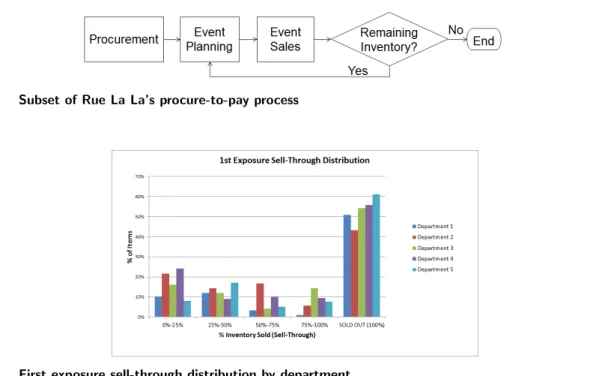
Figure 3 highlights a few aspects of Rue La La’s procure-to-pay process that are critical in understanding the work presented in this paper. First, merchants procure items from designers who typically ship the items immediately to Rue La La’s warehouse1. On a frequent periodic basis, merchants identify opportunities for future events based on available styles in inventory, customer needs, etc.; determining which styles are sold in the event, the price of each style, and when the event starts and ends are all part of what is called the “event planning” process. When the event starts, customers place orders, and Rue La La ships items from its warehouse to the customers. When the event ends or an item runs out of inventory, customers may no longer place an order for that item. If there is remaining inventory at the end of the event, then the merchants will plan
Figure 3 Subset of Rue La La’s procure-to-pay process
Figure 4 First exposure sell-through distribution by department
a subsequent event where they will sell the same style2. We will refer to styles being sold for the first time as “first exposure styles”; a majority of Rue La La’s revenue comes from first exposure styles, and hundreds of first exposure styles are offered on a daily basis.
One of Rue La La’s main challenges is pricing and predicting demand for these first exposure styles. Figure 4 shows a histogram of the sell-through (% of inventory sold) distribution for first exposure items in Rue La La’s top 5 departments (with respect to quantity sold). For example, 51% of first exposure items in Department 1 sell out before the end of the event, and 10% sell less than 25% of their inventory. Department names are hidden and data disguised in order to protect confidentiality. A large percent of first exposure items sell out before the sales period is over, suggesting that it may be possible to raise prices on these items while still achieving high sell-through; on the other hand, many first exposure items sell less than half of their inventory by the end of the sales period, suggesting that the price may have been too high. These observations motivate the development of a pricing decision support tool, allowing Rue La La to take advantage of available data in order to maximize revenue from first exposure sales.
Our approach is two-fold and begins with developing a demand prediction model for first expo-sure items; we then use this demand prediction data as input into a price optimization model to maximize revenue. The two biggest challenges faced when building our demand prediction model include estimating lost sales due to stockouts, and predicting demand for items that have no histori-cal sales data. We use clustering and machine learning regression models to address these challenges and predict future demand. Regression trees an intuitive, yet nonparametric regression model -prove to be the best predictors of demand in terms of both predictability and interpretability.
We then formulate a price optimization model to maximize revenue from first exposure styles, using demand predictions from the regression trees as inputs. In this case, the biggest challenge we face is that each style’s demand depends on the price of competing styles, which restricts us from solving a price optimization problem individually for each style and leads to an exponential number of variables. Furthermore, the non-parametric structure of regression trees makes this problem particularly difficult to solve. We develop a novel reformulation of the price optimization problem and create and implement an efficient algorithm that allows Rue La La to optimize prices on a daily basis for the next day’s sales. Results from a recent field experiment estimate that Rue La La can achieve an increase in revenue of first exposure styles in the test group by approximately 10%, significantly impacting their bottom line.
In the remainder of this section, we provide a literature review on related research and describe Rue La La’s legacy pricing process. Section 2 includes details on the demand prediction model, while Section 3 describes the price optimization model and the efficient algorithm we developed to solve it. Details on the implementation of our pricing decision support tool and integration with Rue La La’s business processes and ERP system, as well as an analysis of the impact of our tool, are included in Section 4. Section 5 presents additional insights from our work with Rue La La that may be applicable to other researchers and practitioners. Finally, Section 6 concludes the paper with a summary of our results and potential areas for future work.
1.1. Literature Review
There has been significant research conducted on price-based revenue management over the past few decades; see ¨Ozer and Phillips (2012) and Talluri and Van Ryzin (2005) for an excellent in-depth overview of such work. The distinguishing features of our work in this field include (i) the development and implementation of a pricing decision support tool for an online retailer offering “flash sales”, (ii) the creation of a new model and theory around multi-product static price op-timization used to set initial prices, and (iii) the use of a non-parametric multi-product demand prediction model.
A group of researchers have worked on the development and implementation of pricing deci-sion support tools for retailers. For example, Caro and Gallien (2012) implement a markdown multi-product pricing decision support tool for fast-fashion retailer, Zara; markdown pricing is common in fashion retailing where retailers aim to sell all of their inventory by the end of relatively short product life cycles. Smith and Achabal (1998) provide another example of the development and implementation of a markdown pricing decision support tool. Other pricing decision support tools focus on recommending promotion pricing strategies (e.g. see Natter et al. (2007) and Wu et al. (2013)); promotion pricing is common in consumer packaged goods to increase demand of
a particular brand. Over the last decade, several software firms have introduced revenue manage-ment software to help retailers make pricing decisions; much of the available software currently focuses on promotion and markdown price optimization. Academic research on retail price-based revenue management also focuses on promotion and markdown dynamic price optimization. ¨Ozer and Phillips (2012), Talluri and Van Ryzin (2005), Elmaghraby and Keskinocak (2003), and Bitran and Caldentey (2003) provide a good overview of this literature.
Unfortunately, Rue La La’s flash sales business model is not well-suited for dynamic price op-timization and is thus unable to benefit from these great advances in research and software tools. There are several characteristics of the online flash sales industry that make a single-price, static model more applicable. For example, many designers require that Rue La La limit the frequency of events which sell their brand in order not to degrade the value of the brand. Even without such constraints placed by designers, flash sales businesses usually do not show the same styles too frequently in order to increase scarcity value and entice customers to visit their website on a daily basis, inducing myopic customer behavior. Therefore, any unsold items at the end of an event are typically held for some period of time before another event is created to sell the leftover items. To further complicate future event planning, purchasing decisions for new styles that would compete against today’s leftover inventory have typically not yet been made. Ostapenko (2013) provides a good overview of this industry’s characteristics.
Since the popularity and competitive landscape for a particular style in the future - and thus fu-ture demand and revenue - is very difficult to predict, a single-price model that maximizes revenue given the current landscape is appropriate. Relatively little research has been devoted to multi-product single-price optimization models in the retail industry. Exceptions include work by Little and Shapiro (1980) and Reibstein and Gatignon (1984) that highlight the importance of concur-rently pricing competing products in a retail environment in order to maximize the profitability of the entire product line. Birge et al. (1998) determine optimal single-price strategies of two substi-tutable products given capacity constraints, Maddah and Bish (2007) analyze both static pricing and inventory decisions for multiple competing products, and Choi (2007) addresses the issue of setting initial prices of fashion items using market information from pre-season sales. The recent survey paper by Soon (2011) provides more examples and a literature review of multi-product pricing models in different settings.
In the literature, demand is modeled as a parametric function of price and possibly other market-ing variables. See Talluri and Van Ryzin (2005) for an overview of multi-product demand functions that are typically used in price optimization. One reason for the popularity of these demand func-tions as an input to price optimization is their set of properties, such as linearity, concavity and increasing differences, that leads to simpler, tractable optimization problems that can provide man-agerial insights. In Section 2, we will be testing some of these functions as possible forecasting
models using Rue La La’s data. In addition, we choose not to initially restrict ourselves to the type of demand functions that would lead to simpler, tractable price optimization problems. Rather, we find the best demand model possible - with respect to both predictability and interpretability - over a wider set of potential demand prediction models. We show that in fact a non-parametric demand prediction model works best for Rue La La, and we resolve the structural challenges that this introduces to the price optimization problem.
1.2. Legacy Pricing Process
For many retailers, initial prices are typically based on some combination of the following crite-ria: percentage markup on cost, competitors’ pricing, and the merchants’ judgement/feel for the best price of the product (see Subrahmanyan (2000), Levy et al. (2004), and S¸en (2008)). These techniques are quite simple and none require style-level demand forecasting.
Rue La La typically applies a fixed percentage markup on cost for each of its styles and compares this to competitors’ pricing of identical styles on the day of the event; they choose whichever price is lowest in order to guarantee that they offer the best deal in the market to their customers. Interestingly, Rue La La typically does not find identical products for sale on other competitors’ websites, and thus the fixed percentage markup is applied. This is simply because other flash sales sites are unlikely to be selling the same product on the same day (if ever), and other retailers are unlikely to offer deep discounts of the same product and at the same time.
In the rest of this paper, we show that applying machine learning and optimization techniques to these initial pricing decisions - while maintaining Rue La La’s value proposition - can have a huge financial impact on the company.
2.
Demand Prediction Model
A key requirement for our pricing decision support tool is the ability to accurately predict demand. To do so, the first decision we need to make is the level of detail in which to aggregate our forecasts. We chose to aggregate items at the style level - essentially aggregating all sizes of an otherwise identical product - and predict demand for each style; the main reason why we do this is because pricing is set by style. Also, further aggregating styles into a more general level of the product hierarchy would eliminate our ability to measure the effects of competing styles’ prices and presence in the assortment on the demand of each style.
The first challenge we face is the lack of historical sales data for first exposure styles. Section 2.1 outlines the data that we have and summarizes the regressors that we developed from this data. A second challenge that typically arises in predicting demand is how to estimate lost sales due to stockouts; we discuss this issue in Section 2.2 and explain how we correct for lost sales. In Section 2.3, we explain the development of our demand prediction model and offer some insights as to why
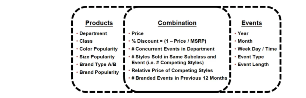
Figure 5 Regressors used to develop demand prediction models
the selected model works well in our setting. We address our third challenge in Section 2.4, which is how to take inventory constraints into account when estimating the portion of demand that we are able to serve given the amount of on-hand inventory (“inventory-constrained demand”).
The final output of our demand prediction model is a prediction of inventory-constrained demand for each first exposure style in a flash sales event. In Section 3, we describe how we use these results as inputs to our price optimization model.
2.1. Data for Prediction Model
Although no historical data exists for first exposure styles, we do have data for other styles sold by Rue La La, and we use this data to develop predictors for our demand prediction model. Specifically, we were provided with sales transactions data from the beginning of 2011 through June 2013, where each data record represents a time-stamped sale of an item during a specific event. This data includes fields such as quantity sold, price, event start date/time, event length, and the inventory of the item at the beginning of the event. We were also provided with product-related data such as the product’s brand, size, color, MSRP (manufacturer’s suggested retail price), and hierarchy classification. With regards to hierarchy classification, each item aggregates (across all sizes) to a style, styles aggregate to form subclasses, subclasses aggregate to form classes, and classes aggregate to formdepartments. For example, all styles of women’s running shoes would be aggregated to the “Women’s Running Shoes” subclass, which is a subset of the “Women’s Athletic Footwear” class, and part of the “Footwear” department.
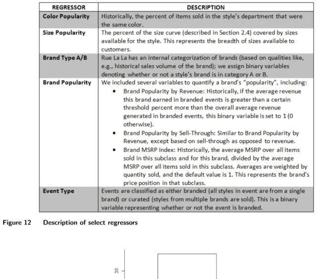
Determining potentially useful predictors of demand that could be derived from this available data was a collaborative process with our main contacts at Rue La La, the COO and the VP of Pricing & Operations Strategy. Together we developed the regressors, i.e., the explanatory variables, for our demand prediction model (summarized in Figure 5). We provide a description for each of the less intuitive regressors in Appendix A. Regressors are calculated for each first exposure style in an event. For the scope of this project, we only consider styles in apparel and accessories departments.
Three of the regressors are related to price. First, we naturally include the price of the style itself as a regressor. Second, we include the percent discount off MSRP as one of our regressors.
Finally, we include a measure for the relative price of competing styles, where we define competing styles as styles in the same subclass and event. This metric is calculated as the price of the style divided by the average price of all competing styles; this input is meant to capture how a style’s demand changes with the price of competing styles shown on the same page. Section 5.2 gives a more in-depth discussion of this regressor and its relation to the marketing literature.
2.2. Estimating Lost Sales
This section focuses on the response for our prediction model - demand for each first exposure style in an event. Although sales quantity is a natural choice for demand, it does not always represent true demand because of potential lost sales due to stockouts. If all of an item’s inventory is sold before the event ends, Rue La La lists the item as “Sold Out” on their website, and no more sales can be recorded for this item. Therefore, sales for an item is the minimum of its demand and inventory. As Figure 4 illustrates, a large percent of Rue La La’s first exposure items sell out before the end of the event, thus the issue of lost sales is frequent in this setting. In fact, many items sell out within just the first few hours of an event.
Almost all retailers face the issue of lost sales, and there has been considerable work done in this area to quantify the metric; see Section 9.4 in Talluri and Van Ryzin (2005) and Anupindi et al. (1998) for an overview of common methods. When we began our work with Rue La La, they already had a method to estimate lost sales that utilized their knowledge of when each sale occurred during the event and, therefore, the remaining time in the event after an item had sold out. The more common methods in the literature either do not use this wealth of data or make limiting assumptions that do not apply in our setting, such as, for example, assuming customer arrivals follow a Poisson process or assuming a customer would not have purchased more than one item. Thus, we decided to use Rue La La’s intuitive and relatively simple method as a starting point and make improvements from there.
Rue La La’s initial estimation method used sales data from items that did not sell out (i.e. when sales = demand) to predict lost sales of items that did sell out. For each event length - ranging from 1 to 4 days - they aggregated hourly sales over all items that did not sell out in their event. Then they calculated the percent of sales that occurred in each hour of the event which gave an empirical distribution - one for each event length - of the proportion of an item’s sales that occur in the first X hours of its event, referred to internally as a “demand curve”. To predict the demand for an item that did sell out, they would identify the time that the item sold out and use this empirical distribution to estimate the proportion of sales that typically occur within that amount of time. By simply dividing the number of units sold (i.e. inventory of that item) by this proportion, they would get a demand estimate for that item had its sales not been constrained by inventory (“unconstrained demand”).
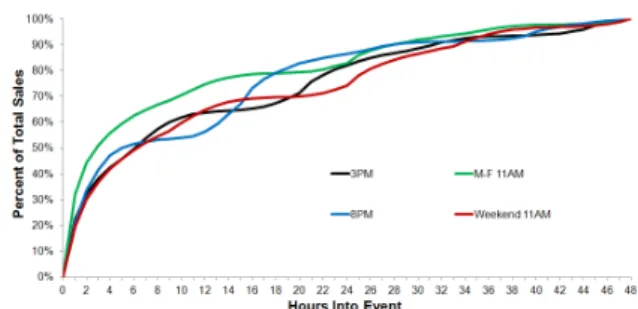
Figure 6 Demand curves for 2-day events
Given knowledge of typical customer behavior on their site, we believed that there was room for improvement in their initial method. For example, almost all of their events start at either 11:00am or 3:00pm during the weekdays and 8:00pm on Sundays, and peaks in traffic on their website follow this same pattern, particularly at the most common 11:00am event start time. Thus we hypothesized that the event start time is also an important factor in estimating an item’s demand curve. To address this type of observation, we decided to use clustering techniques to identify a reasonable number of demand curves to better represent each item, rather than use Rue La La’s initial method with only 4 demand curves, one for each event length.
With the help of our contacts at Rue La La, we identified additional potential factors that we thought could lead to different demand curves: event start time of day, event start day of week, and department. We created a demand curve for each combination of factors and event length; this led to nearly 1,000 demand curves, although many of these curves were built from sales of just a few items. To identify how to further aggregate the factors to create the fewest distinct and interpretable demand curves, we performed hierarchical clustering on the proportion of sales that occurred in each hour. Although a complete review of clustering techniques is beyond the scope of this paper, we briefly summarize the methodology that we used in Appendix B; see Everitt et al. (2011) for more details on cluster analysis.
Figure 6 shows the resulting categorizations that we made via clustering for 2-day events, as well as their associated demand curves. As the figure shows, each curve is relatively steep at the corresponding hours into the event that an 11:00am event starts and flattens out in the very early morning hours. A similar analysis was done for the other possible event lengths and similar insights were made; for 4-day events, a couple of departments warranted their own demand curves, too.
As described above, to predict the unconstrained demand for an item that sold out, we divide the number of units sold by the value of the demand curve at the hour the stockout occurred. Since a style is an aggregation of items that differ only by size, the estimated demand for a style is simply the sum of unconstrained demand across all sizes available in that style.
Figure 7 Illustrative example of a regression tree
2.3. Demand Prediction Model
We developed a separate regression model for each department since styles sold in each department are considered to target a different customer need; thus, demand for these styles as a function of regressors could behave very differently. We performed the analysis in this section separately for each department.
In order to test and compare multiple regression models, we first randomly split the data into training and testing data sets, and we used 5-fold cross-validation on the training data to assist in our model selection process; refer to Section 7.10 in Hastie et al. (2009) for details on cross-validation. We built commonly used regression models with properties as described in Section 1.1, as well as several other models including regression trees, a non-parametric approach to predicting demand. We chose to focus on models which are easily interpretable for managers and merchants at Rue La La in order to better ensure the tool’s adoption3. Although other models, such as neural networks, have become popular in practice in many fields, we decided not to test these types of regression models to avoid giving Rue La La a “black box” demand prediction model.
Surprisingly, regression trees with bagging consistently had the best performance across all de-partments, so we briefly explain this technique and refer the reader to Hastie et al. (2009) for a more detailed discussion. See Figure 7 for an illustrative example of a regression tree. To predict demand using this tree, begin at the top of the tree and ask “Is the price of this style less than $100?”. If yes, then move down the left side of the tree and ask “Is the relative price of competing styles less than 0.8 (i.e. is the price of this style less than 80% of the average price of competing styles)?”. If yes, then the unconstrained demand prediction is 50 units; otherwise, the unconstrained demand prediction is 40 units. If the price is greater than or equal to $100, then the unconstrained demand prediction is 30 units. Given this simple structure, regression trees are considered to be easily interpretable, especially to people with no prior knowledge of regression techniques, as the modeler can trace the process of building the tree and show how results are obtained.
In reality, a regression tree for a department will have several more branches than the one shown in Figure 7. One criticism of regression trees is that they are prone to overfitting from growing the tree too large; we address this issue in two ways. First, we prune our regression tree using tuning parameters found via cross-validation. Second, we employ a bootstrap aggregating (“bagging”) technique to reduce the variance caused by a single regression tree. To do this, we randomly sample
N records from our training data (with replacement), whereN is the number of observations in our training data; then we developed a regression tree from this set of records. We do this 100 times in order to create 100 regression trees. To use these for prediction, we simply make 100 demand predictions using the 100 regression trees, and take the average as our demand prediction4. It is important to note that there are a few other common ways to address the issue of overfitting in regression trees, perhaps the most common of which is using random forests. We chose to use bagging instead of random forests purely from an interpretability standpoint.
We find it very interesting that for every department, regression trees with bagging provides the best demand prediction model compared to all of the models we tested, including the most common models used in previous research in the field. Talluri and Van Ryzin (2005) even comment that to the best of their knowledge, non-parametric forecasting methods such as regression trees are not used in revenue management applications, primarily because they require a lot of data to implement and do a poor job extrapolating situations new to the business. In our case, Rue La La’s business model permits a data-rich environment, and although they offer a huge variety of different styles, there is not much variability in the data for each regressor. Furthermore, in Section 4.1 we describe constraints that we place on the set of possible prices for each style, which have the added benefit of avoiding extrapolation issues. Thus, we believe that the concerns of such non-parametric models like regression trees are mitigated in this environment.
The obvious benefit of using regression trees is that they do not require specification of a certain functional, parametric form between regressors and demand; the model is more general in this sense. In some respect, regression trees are able to determine - for each new style to be priced - the key characteristics of that style that will best predict demand, and they use the demand of styles sold in the past that also had those same key characteristics as an estimate of future demand. While this is effective in predicting demand, unfortunately this non-parametric structure leads to a more difficult price optimization problem, as we will describe in Section 3.
2.4. Applying Inventory Constraints
At this point, it is worth noting the distinction between a demand prediction for a certain style and its inventory-constrained demand prediction. For example, consider a demand prediction of 100 units for a particular item. If we have at least 100 units of that item in inventory, then we would expect to sell all 100 units, i.e. the inventory-constrained demand prediction would also be 100 units. However, if we only have 50 units of that item in inventory, the inventory-constrained demand prediction would only be 50 units. The complication that arises in our model is that inventory is held for each size in the style, yet our demand predictions are for the style.
We transform our demand predictions into inventory-constrained demand predictions by apply-ing inventory constraints on the demand for each size in a style. First, we take a style’sunconstrained
demand prediction and use it to estimate the unconstrained demand for each size. To do this, we used historical data and Rue La La’s expertise to build size curves for each type of product; a size curve represents the percent of style demand that should be allocated to each size. As a simple example of how to apply a size curve, say there are only two sizes of men’s t-shirts, small and medium, and the size curve estimates that 40% of demand is for size small and the other 60% is for size medium. If unconstrained demand is 100 units for the style, then we would predict uncon-strained demand to be 40 units for size small and 60 units for size medium. Inventory constraints are then applied by taking the minimum of each size’s unconstrained demand and inventory. In our example, say we have 50 units in inventory of each size; our inventory-constrained demand would be 40 units for size small and 50 units for size medium. Finally, our inventory-constrained demand for the style is the sum of the inventory-constrained demand for each size. In our example, the inventory-constrained demand for the style is 90 units; note that if we simply applied the 100 units of inventory to constrain demand at the style as opposed to looking at each size’s demand -we would have predicted inventory-constrained demand of 100 units. We do this entire procedure for the prediction made by each of the 100 regression trees and then take the average to get an estimate of the inventory-constrained demand for each style.
The motivation of constraining demand by inventory is closely related to the broken assortment effect studied in the literature (see Smith and Achabal (1998) and Talluri and Van Ryzin (2005)). The broken assortment effect refers to the well-accepted belief that the demand rate of a style decreases when inventory drops below a certain level, presumably because the popular sizes have already stocked out and remaining inventory consists of the less popular sizes. We directly address this issue by quantifying how the style’s demand is affected by having inventory of popular (or unpopular) sizes, rather than using the style’s inventory to estimate an aggregate effect on demand.
3.
Price Optimization
Rue La La typically does not have the ability to buy inventory based on expected demand; rather, their purchasing decision is usually a binary “buy / no buy” decision based on what assortment of styles and sizes a designer may offer them. Because of this, our focus is on using the demand prediction models to determine an optimal pricing strategy that maximizes revenue, given pre-determined purchasing and assortment decisions.
As Figure 5 shows, several regressors are used to build the demand prediction models; however, only three of them are related to price - price, discount, and relative price of competing styles. Recall that the relative price of competing styles is calculated as the price of the style divided by the average price of all styles in the same subclass and event. This input is meant to capture how a style’s demand changes with the price of competing styles shown on the same page. One of the main challenges in converting the demand prediction models to a pricing decision support
tool arises from this input, which implies that the demand of a given style is dependent upon the price of every style sold in the same subclass and in the same event; we will call such styles “competing styles”. Thus, we cannot set prices of each style in isolation; instead, we need to make pricing decisions concurrently for all competing styles. Depending on the department, the number of competing styles could be as large as several hundred. An additional level of complexity stems from the fact that the relationship between demand and price is nonlinear and non-concave/convex due to the regression tree demand prediction models, making it difficult to exploit a well-behaved structure to simplify the problem.
Let N be the number of styles in a given subclass and event, and let M be the set of possible prices for each style withM=|M|representing the number of possible prices. We assume without loss of generality that each style has the same set of possible prices. As is common for many discount retailers, Rue La La typically chooses prices that end in 4.90 or 9.90 (i.e. $24.90 or $119.90). The set of possible prices is characterized by a lower bound and an upper bound and every increment of 5 prices inbetween; for example, if the lower bound of a style’s price is $24.90 and the upper bound is $44.90, then the set of possible prices isM={$24.90,$29.90,$34.90,$39.90,$44.90}, andM= 5. In Section 4, we will discuss how the lower bound and upper bound for each style is selected. Let
pj represent thejth possible price in set M, where j= 1, ..., M.
The objective of the pricing optimization problem is to select a price from M for each style in order to maximize the revenue earned from these styles in their first exposure. We recognize that this is a myopic approach as opposed to maximizing revenue over the styles’ lifetime. However, as described in Section 1.1, there are several characteristics of the online fashion sample sales industry that make this approach the most appropriate.
A naive approach to solving the problem would be to calculate the expected revenue for each combination of possible prices assigned to each style. This requires predicting demand for each style given each competing style’s price. Since there are MN possible combinations of prices for
all styles in a given subclass and event, this approach is often computationally intractable. Thus, we need a different approach. In the following section, we formulate our pricing problem as an integer program and make further improvements to this approach in Section 3.2 to efficiently price competing styles concurrently.
3.1. Integer Formulation
A key observation is that the relative price of competing styles dictates that the demand of a style is only dependent on the price of that style and the sum of the prices of all the competing styles,
not the individual prices of each style. Letkrepresent the sum of the prices of all competing styles. For example, consider a given subclass and event with N = 3 styles. All else equal, the relative price of competing styles for the first style would be the same for the price set {$24.90, $29.90,
$39.90}as it would be for the price set {$24.90, $34.90, $34.90}; in each case,k= $94.70, and the relative price of competing styles for the first style is $24k/.390= 0.79. LetK denote the set of possible values ofk, and note that the possible values ofkrange from (N∗minj{pj}) to (N∗maxj{pj}) in
increments of 5. We haveK,|K|=N∗(M−1) + 1.
Define binary variables yi,j,k such that yi,j,k= 1 if style i is assigned price pj when the sum of
prices of all competing styles is k, and yi,j,k= 0 otherwise, for all i= 1, ..., N where i indexes the
style,j= 1, ..., M where j indexes the possible price, and all k∈ K. The uncertainty in our model is given byDi,j,k, a random variable representing the inventory-constrained demand of theithstyle
and jthpossible price when the sum of prices of competing styles is k.
We can write the following integer program, (IP), to find the set of prices that maximizes first exposure revenue: maxX i X j X k pjE[Di,j,k|pj, k]yi,j,k st. X j X k yi,j,k= 1 ∀ i X j yi,j,k− X j yi0,j,k= 0 ∀i, i06=i, k yi,j,k∈ {0,1} ∀ i, j, k
The first set of constraints ensures that each style is assigned exactly one price corresponding to one possible value of the sum of all prices. The second set of constraints guarantees that for a given k, either each style is assigned a single price or no styles receive any price. We can replace E[Di,j,k|pj, k] in the objective with its forecast from our demand prediction model described in
Section 2, evaluated with pj and k; denote this forecast as ˜Di,j,k. Recall from Section 2.4 that
the forecast generated from our demand prediction model provides an estimate for inventory-constrained demand rather than uninventory-constrained demand. In addition Di,j,k follows no particular
functional form ofpj andkthat exhibits properties such as linearity, concavity/convexity, etc. that
are typically used in revenue management to simplify and solve problems.
The total number of variables in (IP) is N M K=N2M(M−1) +N M. Although this is often considerably better than the naive approach in the previous section, in many cases this problem is still too large to solve in a reasonable amount of time. In particular, there may be as many as several hundred competing styles and/or possible prices; we will discuss realistic time requirements in Section 4, but in many instances, this approach still takes too long to solve.
Another approach using integer programming is to fix the value ofkand solve an integer program to find the set of prices that maximizes revenue, requiring that the sum of prices chosen isk; then we could solve such an integer program for each possible value of k∈ K and choose the solution with the maximum objective value. To do this, we define binary variablesxi,j such that xi,j= 1 if
styleiis assigned pricepj, andxi,j= 0 otherwise, for alli= 1, ..., N and j= 1, ..., M. We can write
the following integer program, (IPk):
maxX i X j pjD˜i,j,kxi,j st. X j xi,j= 1 ∀ i X i X j pjxi,j=k xi,j∈ {0,1} ∀i, j
The first set of constraints guarantees that a single price is assigned to each style. The second constraint requires that the sum of prices over all styles must equalk. Note that this problem only hasN M variables, far fewer than were used in (IP), although we would need to solve this problem
K times, one for each possible value ofk.
Notice that (IPk) is very similar to the multiple-choice knapsack problem except that the
constraint P
i
P
jpjxi,j=k is an equality constraint instead of an inequality constraint such as
P
i
P
jpjxi,j≤k. In either formulation, the multiple-choice knapsack problem is known to be
NP-hard. However, in the next section, we present an efficient algorithm to solve this problem to optimality that exploits a special structure of our problem.
3.2. Efficient Algorithm
Consider the following linear programming relaxation, (LPk), to the above (IPk) optimization
model: maxX i X j pjD˜i,j,kxi,j st. X j xi,j= 1 ∀ i X i X j pjxi,j=k 0≤xi,j≤1 ∀ i, j Let z∗
LPk be the optimal objective value of (LPk), and letzIP∗ k be the optimal objective value of
(IPk). The following theorem provides a bound on the difference in the optimal objective values
of (LPk) and (IPk).
Theorem 1. For any k∈ K,
zLP∗ k−z ∗ IPk≤max i n max j {pj ˜ Di,j,k} −min j {pj ˜ Di,j,k} o .
Note that for a given style, maxj{pjD˜i,j,k} −minj{pjD˜i,j,k} is simply the maximum difference
in revenue across all possible prices. The outer maximization in Theorem 1 subsequently chooses this maximum difference across all styles. The key observation is that this bound is not necessarily
increasing with N or M; in fact, the bound depends only on constants associated with a single style!
The proof of Theorem 1 exploits the fact that K is constructed by taking summations over all possible prices of each style. This structure allows us to obtain such a result that the multiple-choice knapsack problem does not permit. We use this structure in an iterative method to show that there exists an optimal solution to (LPk) that contains fractional variables relating to only
one style; the technique has similarities to the iterative algorithm described in Lau et al. (2011). Furthermore, by showing the existence of a feasible integer solution by only changing this style’s fractional variables to binary variables, we obtain the bound in the theorem. A detailed proof is provided in Appendix C.
Next we present our LP Bound Algorithm that utilizes Theorem 1 to solve (IP) to optimality. LetzIP∗ be the optimal objective value of (IP).
Algorithm 1LP Bound Algorithm
1. For each possible value of k... (a) Solve (LPk) to find zLP∗ k.
(b) Calculate the lower bound of z∗
IPk, denoted asLBk: LBk=zLP∗ k−max i n max j {pj ˜ Di,j,k} −min j {pj ˜ Di,j,k} o
2. Sort the possible values of k∈ K in descending order according toz∗
LPk. Let kl represent the
lth possible value ofk in the ordered set; by construction, we havez∗
LPkl≥z
∗
LPkl
+1.
3. Calculate a lower bound for the optimal objective value of (IP), denoted as LB: LB= maxk{LBk}. Set ˆk= arg maxk{LBk}.
4. For l= 1, ..., K
(a) Solve (IPkl).
(b) If z∗
IPkl> LB, then set ˆk=kl and LB=z∗IPˆk, and store the optimal solution. (c) If LB≥z∗
LPkl
+1 orl=K, then terminate the algorithm; otherwise, continue loop.
Theorem 2. LP Bound Algorithm terminates with zIP∗ =zIP∗ ˆ
k. An optimal solution to (IP) is the optimal price assignments given by the solution to (IPˆk).
The proof is straightforward and is presented in Appendix C.
The real benefit of this algorithm is that rather than solving K integer programs - (IPK) ∀k=
1, ..., K - it solvesK linear programming relaxations, one for each of the integer programs. It then uses the bound found in Theorem 1 to limit the number of integer programs that it needs to solve to find the optimal integer solution. Since the bound is independent of problem size, it is especially
tight for large problems where the run-time could be an issue when solving K integer programs. In fact, our analysis indicates that the LP Bound Algorithm very rarely requires more than just a couple integer programs to be run before reaching an optimal solution for (IP).
4.
Implementation and Results
Sections 2 and 3 described in detail our demand prediction and pricing optimization models used to price Rue La La’s first exposure styles. The first part of this section describes how we transformed these two models into a pricing decision support tool that we recently implemented at Rue La La. In Section 4.2, we present the design and results of our recent field experiment that shows an expected increase in first exposure styles’ revenue in the test group of approximately 10%.
4.1. Implementation
In the implementation of our pricing decision support tool, there are a few factors which we have to consider. The first is determining the price range for each style, i.e. the lower bound and upper bound of the set of possible prices described in Section 3. The lower bound on the price is set by the merchants as described in Section 1.2; this is the minimum price that ensures Rue La La can earn a necessary profit per item and guarantees that they have the lowest price in the market. To maintain its market position as the low-cost provider of fashion products, Rue La La provided us a minimum discount percentage off MSRP for each department, which is an upper bound on the style’s price. To further ensure the customer is getting a great deal, we restrict the upper bound to be no more than the maximum of $15 or 15% greater than the lower bound. Thus, the upper bound on the possible set of prices is calculated as
min{(1−minimum discount of f M SRP)∗M SRP,max{lower bound+ 15, lower bound∗1.15}}. In the rare case that this upper bound is less than the lower bound, the upper bound is set equal to the lower bound, i.e. no price change is permitted.
A second factor to consider is the level of integration and automation in which to build the pricing decision support tool. The goal of the tool is to assist Rue La La in decision making without unduly burdening the executives or analysts with additional time and resources required for its execution. As such, after a period of close monitoring and validation of the tool’s output, the pricing decision support tool has been implemented as a fully automated tool. It is run automatically every day, providing price recommendations to merchants for events starting the next day.
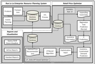
The entire pricing decision support tool is depicted in the architecture diagram in Figure 8. It consists of a Retail Price Optimizer (“RPO”) which is our demand prediction and price optimization component. The input to RPO comes from Rue La La’s Enterprise Resource Planning (ERP) system, which RPO is integrated with; the inputs consist of a set of regressors (“Impending Event
Figure 8 Architecture of pricing decision support tool
Data”) which define the characteristics of the future event required to make demand predictions. This demand prediction process is performed using the statistical tool “R” (www.r-project.org); the 100 regression trees used to predict future demand for each department are stored in RPO, resulting in a more efficient way to make demand predictions. Inventory constraints are then applied to the predictions (from each regression tree) using inventory data for each item obtained from the database. Inventory-constrained demand is then fed to the LP Bound Algorithm developed in Section 3 to obtain an optimal pricing strategy for the event; this is implemented with the lp solve API (lpsolve.sourceforge.net/5.5).
On average, the entire tool takes under one hour to run a day’s worth of events; a typical run requires solving approximately 12 price optimization problems, one for each subclass and event combination for the next day’s events. The longest run-time we encountered for a day’s worth of events was 4.5 hours. These are reasonable run-times given Rue La La is running this tool daily. The output from the RPO is the price recommendation for the merchants, which is also stored in the database for post-event margin analysis.
As the business and competitive landscape changes over time, it is important to update the 100 regression trees stored in R that are used to predict demand. To do this, we have implemented an automated process that pulls historical data from Rue La La’s ERP system and creates 100 new regression trees to use for future predictions in order to guarantee the tool’s effectiveness in the future.
4.2. Field Experiment
Being able to estimate the tool’s impact prior to implementation was key in gaining buy-in and approval from Rue La La executives to use the pricing decision support tool to price first exposure styles. Although not modeled explicitly, Rue La La was particularly concerned that raising prices would decrease demand. One reason for this concern is that Rue La La wants to ensure that their
customers find great value in the products on their site; offering prices too high could lower this perceived value, and Rue La La could experience customer attrition. Another reason for their concern is that a decrease in demand corresponds to an increase in leftover inventory. Since the “flash sales” business model is one that relies on customers perceiving scarcity of each item, an increase in leftover inventory would need to be sold in additional events, which over time could diminish the customers’ perception of scarcity.
Preliminary analysis of the pricing decision support tool on historical data suggested that, in fact, the model recommended price increases had little to no effect on demand5. Motivated by this analysis, we wanted to design an experiment to test whether implementing model recommended price increases would decrease demand. Ideally, we would have liked to design a controlled experi-ment where some customers were offered prices recommended by the tool and others were not; due to potentially inducing negative customer reactions from such an experiment, we decided not to pursue this type of test. Instead, we developed and conducted a field experiment that took place from January through May of 2014 and satisfied Rue La La’s business constraints.
Our goal for the field experiment was to address two questions: (i) would implementing model recommended price increases cause a decrease in demand, and (ii) what impact would the rec-ommended price increases have on revenue? In Section 4.2.1, we describe the design of our field experiment, and we present the results in Section 4.2.2.
4.2.1. Experimental Design
In January 2014, we implemented the pricing decision support tool and began monitoring price recommendations on a daily basis. Note that the lower and upper bounds on each style’s range of possible prices were set as described in Section 4.1; thus, the tool is configured such that it only recommends price increases (or no price change). Over the course of five months, we identified a test set of approximately 1,300{event, subclass}combinations (i.e. sets of competing styles) where the tool recommended price increases for at least one style; this corresponds to approximately 6,000 styles with price increase recommendations. As they were identified, we assigned the set of styles in each {event, subclass}combination which the model recommended price increases to either the “treatment group” or the “control group”. For styles in the treatment group, we accepted the model recommended price increases and raised prices accordingly. For styles in the control group, we did not accept the model recommended price increases and kept the original merchant recommended price as described in Section 1.2.
The assignments to the treatment vs. control groups were made for each {event, subclass} com-bination rather than for each style because optimization results are valid only when price increase recommendations are accepted for all competing styles in the event. We ensured that the set of
styles in the treatment group vs. control group had a similar product mix in terms of characteris-tics such as predicted sell-through (using original prices), inventory, event type, and department. Since price is a key feature of our model and relates directly to our experiment objectives, we decided to further divide both the treatment and control groups into five categories - Category A, B, C, D, and E - based on the actual price of the style. Specifically, all styles in the same category have a similar price, with Category A representing the lowest priced products (price<∼$50) and Category E representing the highest priced products (price > ∼$400). Furthermore, by dividing into categories based on actual price, many of the product mix characteristics (such as average price of competing styles) were naturally similar between the treatment and control groups, too.
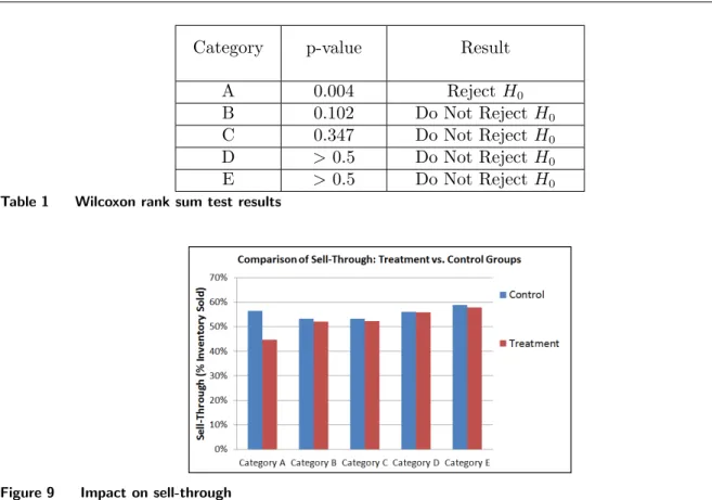
The metric we chose to evaluate the impact of price increases on demand is the sell-through of the style; recall that sell-through is defined as the percent of inventory sold during the event. Intuitively, if price increases cause a decrease in demand, the sell-through of styles in the treatment group should be less than the sell-through of styles in the control group. For each of the five categories, we used the Wilcoxon rank sum test (also known as the Mann-Whitney test) to explore this rigorously. We chose to use this nonparametric test because it makes no assumption on the sell-through data following a particular distributional form, and it is insensitive to outliers. Below we will describe the application of this test to our setting; for more details on the Wilcoxon rank sum test, see Rice (2006).
The null hypothesis (H0) of our test is that raising prices has no effect on sell-through, and this is compared to the one-sided alternative hypothesis that raising prices decreases sell-through. To perform the test, we combined the sell-through data of all of the styles in the treatment and control groups, ordered the data, and assigned a rank to each observation. For example, the smallest sell-through would be assigned rank 1, the second smallest sell-through would be assigned rank 2, etc.; ties were broken by averaging the corresponding ranks. Then we summed the ranks of all of the treatment group observations. If this sum is statistically too low, the sell-through data of the treatment group is significantly less than the sell-through data from the control group and we reject the null hypothesis. Otherwise, we do not reject the null hypothesis, and any difference in sell-through between the treatment and control groups is likely due to chance.
4.2.2. Results
Table 1 presents the p-values of the Wilcoxon rank sum test for each of the five categories6, as well as our decision on whether or not to reject the null hypothesis based on a significance level of α= 10%. Note that for Category A, we would choose to reject the null hypothesis even at the significance level α= 0.5%, whereas for Categories C-E, we would choose not to reject the null hypothesis even at significance levels higher than α= 30%.
Category p-value Result A 0.004 Reject H0 B 0.102 Do Not RejectH0 C 0.347 Do Not RejectH0 D >0.5 Do Not RejectH0 E >0.5 Do Not RejectH0
Table 1 Wilcoxon rank sum test results
Figure 9 Impact on sell-through
These results show that raising prices on the lowest priced styles (styles in Category A) does have a negative impact on sell-through, whereas raising prices on the more expensive styles does not. Figure 9 depicts another, less formal way of comparing sell-through between styles in the treatment and control groups, and similar results are illustrated.
We believe that there are two key factors contributing to these somewhat surprising results. First, since Rue La La offers very deep discounts, they may already be well below customers’ reservation prices (i.e. customers’ “willingness to pay”), such that small changes in price are still perceived as great deals. In these cases, demand is insensitive to price increases. Thus the pricing model finds these opportunities to slightly increase prices without significantly affecting demand; consumers still benefit from a great sale, and Rue La La is also able to maintain a healthy business. Perhaps for the lowest priced styles, the maximum price increase of $15 is too large for consumers to still perceive a great deal, and this may be why we see a negative impact on demand. Rue La La has recently acted on this result and has limited price increases to $5 for styles whose merchant suggested price is less than $50.
A second key factor is that a change in unconstrained demand corresponds to a smaller change in inventory-constrained demand when limited sizes or inventory are available. As a simple example, consider the case where there is only 1 unit of inventory of a particular size. Unconstrained demand for that size may be 10 units when priced at $100 and only 2 units when priced at $110, but
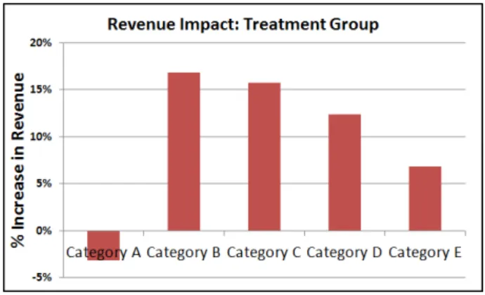
Figure 10 Impact on revenue
have less inventory than the lower priced styles, which suggests that this factor may be contributing to the results we see.
With very little change in sell-through between the treatment and control groups, the treatment group has a big impact on revenue. Figure 10 shows an estimate of the impact on revenue from the treatment group. For Categories B-E, we assume demand is not impacted by the price increases as our results from the Wilcoxon rank sum test suggest. For Category A, results show that demand does decrease due to the price increases; we chose to decrease demand by 21%, which is the average decrease in sell-through as shown in Figure 9. Since the categories are ordered by their associated range of actual prices, although the percent revenue impact is generally decreasing with higher priced categories, thedollar impact on revenue remains quite high.
Overall, we estimate a 10% increase in revenue from using the price recommendations from our tool on the treatment group. It is important to note that the field experiment and model impact assessment that we have presented is based on the model parameters discussed in Section 4.1. If in the future Rue La La is interested in changing these model parameters - for example, to allow for pricedecrease recommendations - new field experiments should be conducted; such changes could positively or negatively affect these results. Finally, it is also important to note that the overall impact on Rue La La’s business depends on the acceptance rate and adherence to the pricing tool’s recommendations.
In summary, our field experiment results show that our pricing decision support tool can have a big impact on Rue La La’s business, resulting in an increase in first exposure styles’ revenue in the treatment group of approximately 10%. Furthermore, the recommended price increases have little impact on demand, resulting in an increase in revenue dollars that drops straight to the bottom line without fundamentally changing Rue La La’s business. Because of this, we are currently using the pricing decision support tool to make price recommendations on hundreds of new styles every day.
Figure 11 Relationship of quantity sold per style to the number of competing styles in an event
5.
Additional Insights and Generalizations
There are several aspects of our work with Rue La La that can extend beyond the flash sales retail environment and we believe could lead to interesting new research directions. In this section, we present a few of those aspects that may be beneficial to both researchers and practitioners. First, we share one of many interesting observations from Rue La La’s historical transactions data regarding assortment planning. Second, we relate the relative price of competing styles to what is known in marketing literature as a “reference price”. Finally, we generalize the theory presented in 3.2 to a special case of the multiple-choice knapsack problem.
5.1. Assortment Planning
In Simchi-Levi (2013), “data-driven research” is introduced as a new paradigm that could be used in conducting operations management research. In fact, the motivation for developing a pricing decision support tool came from analyzing the data and seeing the results shown in Figure 4. We also made many other interesting observations from their data which we believe should be further explored as potential research opportunities. One that we find particularly interesting given its relationship with pricing decisions involves assortment planning. Recall that one of the regressors in our demand prediction model is the number of competing styles sold in an event. Figure 11 shows how the quantity sold per style in an event changes with respect to the number of competing styles in the event, using historical transactions data for one of their departments; the scale on the y-axis has been hidden to protect confidentiality.
As shown in the figure, the quantity sold per style generally seems to increase as the number of competing styles shown in the event increases up to a point around 40 to 50 competing styles -and then quantity sold per style decreases with the number of competing styles. The figure seems to suggest that there may be an “optimal” range of the number of competing styles that should be shown in any given event to maximize the quantity sold of each style, although further research is certainly needed to make such a claim. There are several possible explanations as to why this is the case. For example, demand may be low for events where styles in this department only account
for a small portion of the styles offered and therefore aren’t included in the event’s advertisement. On the other hand, perhaps if there are too many styles shown in a single event, demand for one style starts to cannibalize demand of other competing styles.
Observations such as this one and Rue La La’s interest in identifying business insights and trends from their historical data have motivated the start of a recent project that develops data mining techniques to find such insights and subsequently identify areas of future research in operations management (Johnson et al. (2014)). In the conclusion of this paper, we will discuss several other opportunities for future research.
5.2. Use of Reference Price Metric
Reference prices are standards against which the purchase price of a product is judged (Monroe (1973)). There has been a considerable amount of marketing research that has been conducted that shows the effects of reference prices on consumer purchase behavior; see the survey paper by Mazumdar et al. (2005) for an overview of this literature. A majority of the research has focused primarily on frequently purchased packaged goods, where consumers are thought to use internal reference prices - such as previous purchase prices - to judge the offered price. Research has also shown that consumers use external reference prices - prices or cues explicitly stated by the retailer - to judge prices. Most of the research conducted on the effects of external reference prices is in the context of promotions; examples of such external reference prices include specifying the percent savings or MSRP. Much less research has been done on the use of reference prices for durable goods or new items such as those sold by Rue La La, neither of which permit consumers to use internal reference prices such as previous purchase prices of the same product to judge the offered price. The little research that has been conducted has found that current prices of competitive products and economic trends can be useful consumer reference prices (e.g. Winer (1985); Mazumdar et al. (2005)).
In our demand prediction model, we use the relative price of competing styles to represent the consumer’s reference price. We believe this is an appropriate alternative measure of a reference price that consumers can easily estimate in an online setting such as Rue La La’s, where many competing products and associated prices are displayed on the same page. Emery (1970) suggests that such a metric is indeed used by consumers in price perception, although we have found little research that uses this idea for durable products. Judging by the success of the relative price of competing products in predicting demand, we believe future marketing research would benefit from analyzing consumers’ reaction to this reference price metric, particularly in the online retailing environment.
Finally, our research utilizes reference prices in a new methodological way, regression trees, that to our knowledge has not been explored. Most previous reference price research uses panel data
to infer reference price effects and has a hard time differentiating between reference price effects and other price constructs (Mazumdar et al. (2005)). In our work, though, we show that one can incorporate reference price metrics into machine learning models to explicitly calculate their effect on demand while concurrently taking into account the impact of other price and non-price related factors. Furthermore, we take this demand prediction model one step further and show how managers can ultimately use reference price information to set prices that maximize revenue.
5.3. Special Case of Multiple-Choice Knapsack Problem
As illustrated in Section 3.1, (IPk) is a special case of the multiple-choice knapsack problem, and as
we show in the proof of Theorem 1, this special structure provides a tight bound between (IPk) and
its linear programming relaxation, allowing us to solve (IP) to near-optimality by simply solving linear programming relaxations or to optimality by using the LP Bound Algorithm.
Consider the following more general formulation that has a similar structure as (IPk), (GenIPk):
maxX i X j ci,j,kxi,j st. X j xi,j= 1 ∀ i X i X j ajxi,j=k xi,j∈ {0,1} ∀i, j
where xi,j= 1 if “item” i is assigned “metric” aj, and xi,j= 0 otherwise, for all i= 1, ..., N and
j= 1, ..., M, and where the possible values of k include any summation of N values ofaj. Notice
that this more general problem requires no structural form ofci,j,k; in particular, ci,j,kcan even be
non-monotonic in kand need not be estimated using a regression tree as it was in (IPk).
Let z∗
GenLPk be the optimal objective value of the linear programming relaxation of (GenIPk),
and let z∗
GenIPk be the optimal objective value of (GenIPk). The following theorem provides a
bound on the difference in the optimal objective values of (GenIPk) and its linear programming
relaxation.
Theorem 3. For any possible value ofk,
zGenLP∗ k−z ∗ GenIPk≤max i n max
j {ci,j,k} −minj {ci,j,k}
o
.
The proof of Theorem 3 is nearly identical to that of Theorem 1 and is omitted from the paper. Using this bound, a similar extension can be made to the LP Bound Algorithm and Theorem 2.
6.
Conclusion
In this paper we shared our work with Rue La La on the development and implementation of a pricing decision support tool used to maximize first exposure styles’ revenue. One of the main
development challenges was predicting demand for items that had never been sold before. We found that using regression trees with bagging provided the best demand predictions with respect to both accuracy and interpretability. Unfortunately, the non-parametric structure of this demand prediction model - along with the fact that each style’s demand depends upon the price of all competing styles - led to a seemingly intractable price optimization problem. We developed a novel reformulation of the price optimization problem and created an efficient algorithm to solve this problem on a daily basis to price the first exposure styles in the next day’s events. Results from a recent field experiment used to evaluate our pricing decision support tool show an expected increase in first exposure styles’ revenue in the treatment group of approximately 10%, while minimally impacting aggregate demand. These positive results led to the recent adaptation of our pricing decision support tool for daily use.
There are several key takeaways from our research for both practitioners and academic re-searchers. First, we hope that the success of this pricing decision support tool motivates retailers to investigate similar techniques to help set initial prices of new items. Second, we think that a key observation of our demand prediction model is that a non-parametric regression technique out-performs many of the well-studied parametric demand prediction models in the literature. While this will not necessarily be the case in all situations, we challenge researchers and practitioners to explore new - and possibly less structured - demand prediction models. Finally, our analysis shows that an important regressor in the demand prediction model is the relative price with respect to competing styles, which we describe as closely related to the idea of a reference price.
Of course, the non-parametric nature of our demand prediction model and the dependency of demand on competing styles’ prices pose challenges to subsequently solving a price optimization model. We thus provide new machinery and describe the software architecture we developed that together permit an efficient implementation of such a price optimization problem. The optimization technique is independent of the fact that we used a regression tree or the particular metric for reference price, and we showed that it can be applied in a more general setting.
This paper would not be complete if we did not mention two major research directions that we have begun working on with Rue La La. Throughout this research collaboration with Rue La La, they often asked the question, “What general business insights or trends have you noticed when looking at our data?”. For instance, one such insight we noticed was shared in Section 5.1 regarding how the number of competing styles in the assortment was related to the quantity sold per style. Unfortunately, we did not have a systematic way of identifying trends in the data, which led us to recently start a new project to develop data mining techniques to find such insights (Johnson et al. (2014)). Our goal is not only to find business insights or trends, but also to subsequently identify and pursue new areas of operations management research.
Another interesting research question motivated by the Rue La La data is related to how much additional revenue could be made by allowing the price of styles to change during the event. Rue La La’s concern in allowing prices to change during an event is that they believe too many price changes will cause confusion and a negative perception amongst customers. With that said, Simchi-Levi et al. (2013) show in a similar setting that in fact much of the benefit achieved by changing prices can be accomplished with just a single price change. Preliminary analysis suggests that the accuracy of the unconstrained demand prediction is substantially better if the prediction is made one hour into the start of the event and includes information about the quantity sold in the first hour. This motivated Rue La La to consider a single price change during the first hour of the event to improve forecast accuracy and calibrate prices to better match remaining inventory with demand. Thus, it would be interesting to combine the techniques of this paper and the learning and optimization techniques from Simchi-Levi et al. (2013) to further improve Rue La La’s revenue.
Endnotes
1. In some cases, the contract is such that the designer commits to selling up to X units of an item to Rue La La in a given time window, but Rue La La is not committed to purchasing anything. In this case, Rue La La plans an event within the time window, receives customer orders up to X units, and then purchases the quantity it has sold. There are a few changes to the model and implementation steps due to this type of contract, but for ease of exposition they have been left out of the paper.
2. Returns re-enter the process flow at this point and are treated as remaining inventory.
3. Models tested included least squares regression, principal components regression, partial least squares regression, power/multiplicative regression, semilogarithmic regression, and regression trees.
4. We make a slight adjustment to this approach which will be described in Section 2.4. 5. A discussion of this historical analysis has been left out for brevity.
6. We used the approximation presented below Table 8 of Appendix B in Rice (2006) to calculate the critical values.
Acknowledgments
We thank Murali Narayanaswamy, the Vice President of Pricing & Operations Strategy at Rue La La, Jonathan Waggoner, the Chief Operating Officer at Rue La La, and Philip Roizin, the Chief Financial Officer at Rue La La, for their continuing support, sharing valuable business expertise through numerous discussions, and providing us with a considerable amount of time and resources to ensure a successful project. The integration of our pricing decision support tool with their ERP system could not have been done without the help of Hemant Pariawala and Debadatta Mohanty. We also thank the numerous other Rue La La executives and employees for their assistance and support throughout our project. This research also benefitted from
discussions with Roy Welsch (MIT), ¨Ozalp ¨Ozer (UT Dallas), Matt O’Kane (Accenture), and students in David Simchi-Levi’s research group at MIT. Finally, we thank the Accenture and MIT Alliance in Business Analytics for funding this project.