Trade in value added and factors: A comprehensive approach

(1)

Trade in value added and factors: A comprehensive approach

Neil Foster?, Robert Stehrer?, and Gaaitzen de Vries∗ ?_{The Vienna Institute for International}

Economic Studies (wiiw) Rahlgasse 3, A-1060 Vienna, Austria.

∗ _{University of Groningen (RUG)}

9700 AB Groningen, The Netherlands.

Version: August 3, 2011

This paper was written within the 7th EU-framework project ’WIOD: World Input-Output Database: Construction and Applications’ (www.wiod.org) under Theme 8: Socio-Economic Sciences and Hu-manities, Grant agreement no. 225 281.

(2)

Abstract

Based on recent approaches to measuring the factor content of trade when intermediates are traded we decompose value added trade and its components (capital and labor, as well as their subcomponents ICT and Non-ICT capital and educational attainment categories) distinguishing between various categories of foreign value added content of exports and imports. We add to the literature by simultaneously con-sidering both exports and imports allowing for a focus on the patterns and dynamics of net value added trade and its components rather than vertical specialization patterns based on exports only. We show that a country’s trade balance in value added equals its trade balance in gross trade. Empirically we present results of an application of the proposed decomposition method based on the recently compiled World Input-Output Database (WIOD) covering 40 countries and 35 industries over the period 1995-2006. We show that the domestic value added content of exports and the foreign value added content of bilateral trade dominates, but that the foreign or multilateral part is increasing over time pointing towards increas-ing international integration of production. We add a discussion of the trade balances with respect to production factors in value terms providing a distinct view on the patterns of trade deficits and surpluses across countries.

Keywords: value added trade; trade in factors; trade integration; vertical specialization; production net-works

(3)

TRADE IN VALUE ADDED AND FACTORS: A

COMPREHENSIVE APPROACH1

1 Introduction

Trade in value added has become an increasingly debated topic due to the rapid integration of production processes and the further inclusion of countries in this process. Though this process has been ongoing for quite some time there have been rapid integration processes in the world economy taking place over the last decade or so. In the 1990s this was the creation of the North American Free Trade Agreement (NAFTA) concerning the US, Canada and Mexico and the integration of formerly communist countries with Western EU countries which started after the transformational recession in these countries and led to the accession of some countries into the European Union in 2004. Further, large developing countries such as Brazil, Russia, India and China (and Indonesia and South Africa to a lesser extent) - termed the BRIC, BRIIC, or BRICS countries - became important players on world markets at least in particular industries. This implied an increase in overall trade flows in the world economy with increasing shares of imports and exports between these newly integrating countries and the developed world. This integration of trade flows in the world economy was further accompanied by increasing foreign direct investment activities. One particular feature of this integration process was also the integration of production struc-tures in the sense that firms offshore activities to other countries to exploit cost advantages in particular stages of production. This integration of production processes has been theoretically analyzed under different headings including ’fragmentation’, ’slicing up the value chain’, ’outsourcing’ and ’offshoring’ or the ’second unbundling’ and recent contributions emphasizing ’trade in tasks’.

From an empirical point of view there is still the challenge to properly measure this ongoing integra-tion of producintegra-tion processes. The literature ranges from particular case studies for products like the Bar-bie doll (Tempest, 1996), the iPod (Linden et al., 2009; Varian, 2007), computers (Kraemer and Dedrick, 2002), or the Nokia N95 (Ali-Yrkko¨o, 2010) or more complex products like cars (Baldwin, 2009) or airplanes (Grossman and Rossi-Hansberg, 2008), to studies of trade patterns in particular products such as ’parts and components’ and overall trade in intermediates versus trade in final goods (Miroudot et al., 2009; Stehrer et al., 2011) and a number of studies focusing on the magnitude and changes of ’vertical

1

Previous versions of the paper have been presented at the ”OECD Working Party on Trade in Goods and Services Statistics (WPTGS)”, September 2010, the WTO Public Forum in 2010, the wiiw Seminar in International Economics in Vienna, May 2010, and the Worldbank workshop on ”The Fragmentation of Global Production and Trade in Value Added - Developing New Measures of Cross-Border Trade”, June 2011, as well as at the WIOD consortium meeting held in May 25-27, 2011, Seville, Spain. We thank the respective participants for useful discussion and suggestions. Further we would like to thank Wolfgang Koller, Austria, for useful comments.

(5)

specialization’ patterns. In the European context the changes in the international structure of production are discussed from a multi-disciplinary point of view in Faust et al. (2004). This book also provides a number of case studies at the level of industries (the automobile industry, the electronics industry, and the apparel industry). Other recent studies focus on measuring trade in value added between countries thus trying to measure how much of value added created in the production process in one country is exported thus ’netting out’ the value already embodied in imported products and the extent of ’vertical specializa-tion’ or ’vertical integraspecializa-tion’ (Hummels et al., 2001; Daudin et al., 2009; Johnson and Noguera, 2009; Koopman et al., 2010), with an overview of these approaches provided by Meng and Yamano (2010); see also Meng et al. (2011) for a decomposition of vertical specialization measures. Related to these are papers on the measurement of trade in value added, examples including Escaith (2008); Maurer and Degain (2010); Timmer et al. (2011). Further there are a number of papers with a focus on the Asian production and trade network (recent examples include Meng and Inomata, 2009; Hiratsuka and Uchida, 2010; Yamano et al., 2010).

In the international trade literature this issue has to some extent been addressed over a number of years with work measuring the factor content of trade flows. The seminal contribution in this respect was that of Vanek (Vanek, 1968) and the so called Heckscher-Ohlin-Vanek model; for a recent overview see (Baldwin, 2008). In this model the perspective switches from that on trade in goods to trade in factors of production embodied in the goods traded. Empirically, this goes back even earlier to the important contribution of Leontief (Leontief, 1953) which triggered a number of subsequent studies focusing on the ’Leontief paradox’. Only recently have there been successful attempts to solve this ’paradox’ by allowing for (Hicks neutral) technology differences across countries (Trefler, 1993). One particular concern in these contributions was to properly account for trade in intermediate products, an issue which has been the focus of some recent contributions including those of Davis and Weinstein (2001), Reimer (2006), and Trefler and Zhu (2010), though this issue was considered earlier by Deardorff (1982) and Staiger (1986).

The starting point of this paper are these recent papers accounting for intermediates trade and in particular the contribution of Trefler and Zhu (2010) where a Vanek-consistent measure of the factor content of trade is proposed. Based on this approach we introduce an alternative approach to decompose trade flows in value added and its components such as ICT and Non-ICT capital and labor differentiated by skills and relate these to recent approaches of measuring vertical specialization patterns (Hummels et al., 2001; Daudin et al., 2009; Johnson and Noguera, 2009; Koopman et al., 2010). Our approach can

(6)

be aligned with the measures of vertical specialization proposed in these studies which will be discussed below. We add to this literature by simultaneously looking at both exports and imports of value added thus focussing on net trade in value added rather than exports or imports of value added separately. The proposed framework also allows to show that a country’s net export in value added equals its net exports in gross trade which aligns this approach to national accounting. We differentiate between domestic and foreign components in value added exports and imports. The data allow us to further break down the figures of (net) trade in value added in to the components of value added. Particularly, we split value added (in value terms) into capital and labor income, and these two into ICT and Non-ICT capital and high, medium and low educated (by ISCED categories) labor income, respectively. The paper thus tries to link the literature on trade in value added and vertical specialization and on the factor content of trade by applying a decomposition approach.2

The paper proceeds as follows. In Section 2 we introduce our method of decomposing trade in value added. Section 3 provides a short overview of the recently compiled world input output database (WIOD) database that we use. Based on this we present selected results in Section 4. Section 5 concludes and points towards further avenues of research.

2 Measuring trade in value added and factors

In this section we introduce our approach to the decomposition of trade flows in value added exports and imports and consequently net trade. The same approach is also used to further to split up these flows into value added components, i.e. the value of labor and capital traded which can be further split up by various categories as outlined below. There is already a wide literature on the measurement of vertical specialization, value added chains and trade in value added (see e.g. Hummels et al., 2001; Johnson and Noguera, 2009; Daudin et al., 2009; Koopman et al., 2010; Timmer et al., 2011).

Often this literature focuses on measuring the vertical integration of production processes focusing on exports and thus leaving out the aspect that all countries are also important importers of intermediates and the existence of two-way trade in intermediates as outlined above.3 On the other hand, the literature focusing on the effects of outsourcing on labor markets (employment and wages) and other variables like productivity often focus on the import side only. In this paper we therefore aim at including both

2

In future research this decomposition can be continued further as will be outlined in the conclusions. 3

The literature focuses on the ’import content ofexports’; using supply-driven IO models allows one to also calculate the ’export content of imports’ (see for example Meng and Yamano, 2010).

(7)

sides of trade to measure the extent of exports, imports and net trade in value added and its relative importance across countries’ trading patterns. The WIOD database (see below) further allows us to follow the respective trends over time and to further decompose value added flows into its components.

Another strand of literature which is related to the issue of trade in value added and vertical special-ization focuses on trade in factors and is often motivated by the Heckscher-Ohlin-Vanek theorem with the further complication when trade in intermediates has to be accounted for (see Deardorff (1982) and Staiger (1986) for early contributions and Reimer (2006) and Trefler and Zhu (2010) for more recent ones). The approach suggested here is motivated by a recent paper on trade in factors, Trefler and Zhu (2010), which focuses on the correct (or ’Vanek consistent’ way) of calculating the factor content of trade with trade in intermediates. We apply a similar method of calculating the factor content with two mod-ifications. First, we apply this approach using value added shares in gross output and capital and labor income shares in gross output rather than physical input coefficients which most of the papers focusing on trade in factors is based. In essence, we therefore not only allow for cross-country and cross-industry differences in direct and indirect input coefficients but also for differences in factor rewards.4 Second, we decompose the resulting measure into several categories which are outlined below in detail. In particular, this latter aspect links this paper to other approaches of measuring vertical integration and trade in value added.

2.1 A comprehensive approach

The starting point for the analysis are indicators of the share of value added in gross output denoted by vector v, the Leontief inverse of the global input-output matrix, L = (I−A)−1 withAdenoting the coefficients matrix, and the flows of exports and imports of goods between countries denoted byt. For simplicity we first discuss our approach for the case of three countries without an industry dimen-sion. Further, we discuss net trade in value added from the viewpoint of country 1 without any loss in generality. In this special case the vector of value added coefficients becomes v0 = (v1, v2, v3), the Leontief-inverse is of dimension3×3and the trade vector is written ast = (x1∗,−x21,−x31) where

x1∗ =P

p,p6=1x1pdenotes exports of country 1 to all countries andxr1denotes exports of countryrto 1, i.e. imports of country 1. These imports are included in negative terms which results in net trade of value added for country 1, i.e. tV = v0Lt. For the decomposition procedure however we need the individual

entries of the matrix capturing exports and imports of country 1 which is achieved by a diagonalization

4

This can later be decomposed into the effects of changes in productivity, factor rewards and trade patterns by splitting ratios over gross output into factor rewards and physical input coefficients, i.e. to disentangle quantity and factor price effects.

(8)

of the value added coefficients and trade vector which results in the following exposition: T1_V =      v1 ₀ ₀ 0 v2 0 0 0 v3           l11 _l12 _l13 l21 l22 l23 l31 _l32 _l33           x1∗ 0 0 0 −x21 0 0 0 −x31      =      v1l11x1∗ −v1l12x21 −v1l13x31 v2l21x1∗ −v2l22x21 −v2l23x31 v3l31x1∗ −v3l32x21 −v3l33x31     

The first matrix contains the value added coefficients of the three countries, the second matrix denotes the elements of the Leontief inverse from the global input-output matrix and the last matrix contains exports of country 1 and imports of country 1 from the other countries which are included as negative values. Summing up this matrix over rows and columns therefore gives a measure of net trade of value added for country 1. One should note however that this also includes indirect flows of value added and imports and it is therefore advisable to discuss the entries in these matrix separately. This will also document the decomposition of value added exports and imports in its various forms.

• Exports: The first column in matrixT1_V describes value added exports of country 1.

∗ Domestic value added content of exports: The first entry,v1l11x1∗, denotes total direct and indirect value added exports of country 1 to all other countries.

∗ Foreign value added content of exports: The production of these exports also requires inputs from other countries. For production of these inputs used to produce exports of country 1 -value added in the other countries is created. This is captured by the remaining terms in the first column by partner country, i.e.P

p,p6=1vplp1x1∗. Note, that this is added to value added exports of country 1, though value added is created in the other countries.

• Imports: The other columns capture the value added content of country 1’s imports.

∗ Foreign value added content of bilateral imports: The exports of country 2 to country 1 embody value added from the second country. Thus the second term in the second column captures country 1’s value added imports from country 2. Similarly, the third entry in the third column captures the value added imports from country 3. Generally, the elements of the diagonal in the import block contain bilateral value added imports,−P

(9)

∗ Re-Imports: Exports of country 2 to country 1 can also require inputs from country 1 itself. Therefore, the first entry in column 2 captures value added imports of country 1 embodied in imports from country 2; analogously for the third term in the first row. Total re-imports of value added are therefore−P

p6=1v1l1pxp1.

∗ Foreign multilateral value added content of imports: Country 2’s exports to country 1 also require inputs from other countries. Thus, for example the entry in row 3 of column 2 cap-tures the value added imports of country 1 from country 3 which are embodied in imports from country 2. An analogous interpretation holds for the entry in row 2 of column 3. Thus, the total amount of these imports is given by−P

p,q,p6=q;p,q6=1vqlqpxp1.

Analogous interpretations would also hold for countries 2 and 3 and generally for N countries. To disentangle these five components of net value added trade for country 1 it is convenient to rewrite the sum of the equation in the following way:

tr_V = X s,s6=r vrlrrxrs | {z } Domestic + X s,s6=r X p,p6=r vplprxrs | {z } Foreign | {z }

Value added content of exports

− X p6=r vplppxpr | {z } Bilateral + X p,q,p6=q;p,q6=r vqlqpxpr | {z } Re-imports +X r6=p vrlrpxpr | {z } Multilateral | {z }

Value added content of imports

(1)

There is a close relationship of this measure to others on vertical specialization already existing in the literature. Koopman et al. (2010) sorts out the measures as supposed by Hummels et al. (2001), Johnson and Noguera (2009) and Daudin et al. (2009) and provided an explicit derivation of the VS1 measure as supposed by Hummels et al. (2001). Relying on these results we can interpret the five terms in the above equation accordingly: The first term is country 1’s domestic value added in direct exports, the second is the ’true’ VS11 measure capturing the import content of exports (see Hummels et al., 2001; Koopman et al., 2010), the third term are country 1’s direct imports of value added or the other countries’ direct exports of value added to country 1 (where each import of country 1 is valued with the trading partner’s value added coefficients), the fourth term is the VS1∗1measure capturing the re-imported value added of exports (see Daudin et al., 2009; Koopman et al., 2010) and the last term are country 1’s indirect value added imports through third countries which is therefore the sum of VS1pmeasures (see Hummels et al., 2001) where this was derived as value added exports through third countries (see also Koopman et al., 2010, where this was derived explitely).

(10)

Extending the above framework to many sectors requires only some slight modifications in the di-mensionality of the matrices involved. Let N denote the number of countries and G the number of industries. Tr

V =vˆ0Lˆtrvis now aN G×1matrix, the Leontief inverseLis of dimensionN G×N G

andtris of dimensionN G×1; with sector specific information on exports (to all countries) and sector specific information of imports from individual countries. Calculations can then be performed in exactly the same way as indicated above with additionally summing up over industries.5 To derive country spe-cific results one first has to add up block-wise. Thus the algebra has to be rewritten in the following way withR =I⊗ιandS = R0denoting summation matrices whereIis the identity matrix of dimension

N ×N andιdenoting a vector of ones of dimensionG×1;⊗denotes the Kronecker symbol. Matrix

Ris therefore of dimensionN G×N. Pre- and post-multiplying the industry specific matrixTr_V which is of dimensionN G×N GbySandRrespectively, results in a matrix of dimensionN×N which has the same interpretation as above (having however incorporated industry-specific interrelations).

2.2 Trade balance in value added and gross trade

Following this approach allows us to show the relationship between a country’s trade balance in gross and value added trade. This is important to look at in detail as in many instances case studies show that a country is running a trade deficit in gross terms of a particular product whereas when taking account of intermediates trade, or considering trade in value added, the trade deficit in value added term is lower or even turns into a trade surplus (see e.g. Linden et al., 2009; Xing and Detert, 2010).

Based on the framework introduced above it can easily be shown that a country’s net trade in value added equals net trade from gross exports and imports (see also Johnson and Noguera, 2009, where this is shown in a2×2 example) From an intuitive point it is clear that total exports in value added of a country must be imported in another country (as all exports of goods must be imported somewhere else). As trade in goods is traced back to primary factor inputs and rewards and the coefficients of direct and indirect value added creation in a closed system is equal to one the trade deficit of a country equals the deficit measured in value added. Thus, this equality is a consequence of national accounting identities in a closed system of world trade. Further, as we view trade deficits from the viewpoint of individual countries we consider exports and imports as a form of final (exogenous) demand.

From an algebraic point of view this can be shown relatively straightforward. The vector of value added, which we will denote by va, can be expressed in the following way from which value added

(11)

coefficients can easily be derived. Value added is gross output minus intermediate inputs,va=q−qAˆ 0ι. Expressed in relation to gross output yields

ˆ

q−1va=v=ˆq−1q−qˆ−1qAˆ 0ι=ι−A0ι

and thereforev0 =ι0(I−A). Inserting into our equation for measuring net trade in value added we get

tnet_V =v0 I−A−1

t=ι0 I−A

I−A−1

t=ι0t=tnet

i.e. net trade in value added equals net trade in goods and services. Similarly one can show (by using trade vectors consisting of the export cell or the import cells) that the ratio of value added exports (imports) to gross exports (imports) equals one. The reason for this result is that in this framework all goods (intermediates and final goods) are produced by capital and labor as the only two primary factors which capture all the value added.

Thus one has carefully to consider the results that a country’s trade deficit in value added might be lower than in terms of gross trade when considering bilateral flows. This might be the case in a bilateral relationship though it is not true when taking trade with all countries into account.6

2.3 Trade in factors

Instead of doing the analysis with the vector of value added coefficientsvwe can now exploit the fact that value added is a composite of income of various factors. Thus given data at hand one might split up each element of the value added coefficients vector into subcomponents like labor and capital, i.e. vr_i =

P

fvi,fr wheref denotes the factors considered. The data set at hand which are described below in more

detail allows us to distinguish first between labor and capital income. The former can be split into three categories by educational attainment levels according to ISCED classification (high, medium, and low educational attainment) and the latter into ICT and Non-ICT capital. This means that we can differentiate trade in value added into trade in capital and labor and the respective categories. These individual factors of value added trade then sum nicely up to the aggregate as described above. Importantly, this allows then to consider in which factors a country is running a trade deficit or surplus. As we will see a country which is running a trade deficit can nonetheless be a net exporter of a particular factor like high-educated labor.

(12)

Summarizing, this approach of measuring net trade in value added is consistent with measures of net trade in gross terms, incorporates other measures as suggested in the recent literature and allows for a decomposition of value added trade along various dimensions which we document in subsequent sections.

3 Socio-economic accounts and World Input-Output Tables

In this section we provide information on a new database that is used to study the factor content of value added trade. For our analysis, we require a dataset on output and the use of production factors by industry including intermediates, as well as a dataset on bilateral trade flows at the same level of industry detail. The former set of data is obtained from Socio-Economic Accounts (SEAs), whereas the latter is derived from national input-output or supply and use tables which are combined into World Input-Output Tables (WIOTs) by use of bilateral trade data. Both datasets can be integrated in an empirical analysis, because we use the National Accounts framework. The information is collected on an annual basis from 1995 to 2006 at a detailed 35 industry level, but may also provide higher level aggregates. The industry classification follows the ISIC revision 3 classification (which is compatible to NACE revision 1.1; see appendix tables for a list of htese industries). Together, the GDP of the 40 countries covered in the database account for about 85 percent of world GDP. The variables from the SEAs include gross output and value added, final demand expenditures, as well as employment by education attainment, and capital compensation. The WIOTs are a combination of national input-output tables in which the use of products is broken down according to their origin. The remainder of this section provides an overview of the construction of the SEAs and the WIOTs.

3.1 Socio-Economic Accounts

The SEAs have largely been constructed on the basis of data from national statistical institutes (NSIs) and processed according to harmonized procedures. These procedures were developed to ensure international comparability of the basic data and to generate socio-economic accounts in a consistent and uniform way. Cross-country harmonization of the basic country data has focused on a number of areas including a common industrial classification, consistent definitions of various labor and capital types, and the use of similar price concepts for inputs and outputs. Importantly, this database is rooted in statistics from the National Accounts and follows the concepts and conventions of the System of National Accounts (SNA)

(13)

framework, and its European equivalent (ESA), in many respects. As a result, the basic statistics can be related to the national accounts statistics published by NSIs, although with adjustments that vary by group of variables considered: output and intermediate inputs, labor input and capital input.

Nominal and price series for output, intermediate inputs, and value added at the industry level are taken directly from the National Accounts. As these series are often short (as revisions are not always taken back in time) different vintages of the national accounts were bridged according to a common link-methodology. In cases where industry detail was missing, additional statistics from censuses and surveys were used to fill the gaps.

Labor service input is based on series of employment and wages of various types of labor. These series are not part of the core set of National Accounts statistics published by NSIs; typically only total employment and wages by industry are available from the National Accounts. For these series additional material has been collected from employment and labor force statistics. We cross-classify employment by educational attainment. For each country, a choice was made of the best statistical source for consistent wage and employment data at the industry level. In most cases this was the labor force survey (LFS), which in a number of cases was combined with earnings surveys as wages often are not included in the LFS. In other instances, an establishment survey, or social-security database was used (Timmer et al., 2007; Erumban et al., 2011).

Most employment surveys are not designed to track developments over time and breaks in method-ology or coverage frequently occur. Therefore, care has been taken to arrive at series which are time consistent. Further, labor compensation of self-employed is not registered in the National Accounts, which, as emphasized by Krueger (1999), leads to an understatement of labor’s share. We make an im-putation by assuming that the compensation per hour of self-employed is equal to the compensation per hour of employees. This is especially important for industries which have a large share of self-employed workers, such as agriculture, trade, business and personal services. Also, we assume the same labor characteristics for self-employed as for employees when information on the former is missing. These assumptions are made at the industry level. Finally, capital compensation is derived as gross value added minus labor compensation.

3.2 World Input-Output Database

In this section we outline the basic concepts and construction of our world input-output tables (WIOTs). Basically, a WIOT is a combination of national input-output tables in which the use of products is broken

(14)

down according to their origin. Each product is produced either by a domestic industry or by a foreign industry. In contrast to the national input-output tables, this information is made explicit in the WIOT. For each country, flows of products both for intermediate and final use are split into domestically produced or imported. In addition, the WIOT shows for imports in which foreign industry the product was produced. As building blocks for the WIOTs, we use national supply and use tables (SUTs) that are the core statistical sources from which NSIs derive national input-output tables. SUTs are a natural starting point as they provide information on both products and industries. Supply tables provide information on products produced by each domestic industry and use tables indicate the use of each product by an industry or final user. The linking with international trade data, that is product based, and factor use that is industry-based, can be naturally made in a SUT framework.

To ensure meaningful analysis over time we start from industry output and final consumption series as described above, and benchmark national SUTs to these time-consistent series. Typically, SUTs are only available for a limited set of years and once released by the national statistical institute revisions are rare. This compromises the consistency and comparability of these tables over time as statistical systems develop, new methodologies and accounting rules are used, classification schemes change and new data becomes available.7 By benchmarking the SUTs on consistent time series from the National Accounting System (NAS), tables can be linked over time in a meaningful way. This is done by using a SUT updating method (the SUT-RAS method) which is akin to the well-known bi-proportional (RAS) updating method for input-output tables as described in Temurshoev and Timmer (2011).

Next, to split the use of domestic production and imports, we rely on import flows of all coun-tries covered in WIOD from all partners in the world at the HS6-digit product level taken from the UN COMTRADE database. Based on the detailed product description at the HS 6-digit level, products are al-located to three use categories: intermediates, final consumption, and investment. The allocation follows from a revised classification of Broad Economic Categories (BEC) as made available from the United Nations Statistics Division (see P¨oschl and Stehrer, 2010). As yet no standardized database on bilateral service flows exists. Services trade data from Balance of Payments statistics have been collected from various sources (including OECD, Eurostat, IMF and WTO), checked for consistency, and integrated into a bilateral service trade database (Francois and Pindyuk, 2010).

International SUTs were constructed using this bilateral trade data by use category. We start from the import vector provided in the supply tables. Import values for each country and product are split up

7

Indonesia, Japan, Korea, and Taiwan only provide input-output tables which have been transformed back into supply and use tables. As a result, we have no information on secondary production in the supply tables for these countries.

(15)

into the three use categories. Next, within each use category a proportionality assumption is applied to split up the imports for each use category across the relevant dimensions. Investment are allocated only to gross fixed capital formation (i.e. not considering changes in inventories and valuables). This resulted in an import use table for each country, where each cell of the import use table is then split up by country of origin.

As a final step, international SUTs are transformed into an industry-by-industry type World Input-Output Table. We use the so-called ”fixed product-sales structure” assumption stating that each product has its own specific sales structure irrespective of the industry where it is produced (see Eurostat, 2008). For the period from 1995 to 2006, this results in a WIOT for 40 countries and 35 industries, i.e. the intermediates demand block is of dimension1400×1400, plus the additional rows on value added and columns on final demand categories.8

In short, we derive time series of national SUTs and link these across countries through detailed international trade statistics to create so-called international SUTs. These international SUTs are used to construct the symmetric world input-output tables.

In the next section we present figures for individual countries grouping them into EU-15, EU-12 plus Turkey, NAFTA (Canada, USA and Mexico), Asian countries (Japan, Korea and Taiwan), and the BRIICs (Brazil, Russia, India, Indonesia and China) to which we also add Australia and Rest of World. One should note however that all calculations are performed at the level of individual countries and industries thus taking all available information into account.9

4 Patterns of trade in value added and factors

In this section we present selected results on the patterns of value added by applying equation (2.1). For this we proceed in a series of steps: First, we present the magnitudes of gross and value added exports and imports and the corresponding net figures for the 41 countries. We then split up trade in value added to its foreign and domestic contents. Finally, Trade in value added is then differentiated by factors. We report results for the years 1995, 2000 and 2005.

8_{The Rest of the World (RoW) is not explicitly modeled in this case but appears only in the import matrices by country} (imports from RoW by product and industry) and export column (exports to rest of the world). We assume the structure of the input coefficients for the RoW is similar to the average coefficients from Brazil, China, India, Indonesia, and Mexico.

9

(16)

4.1 Trade balances

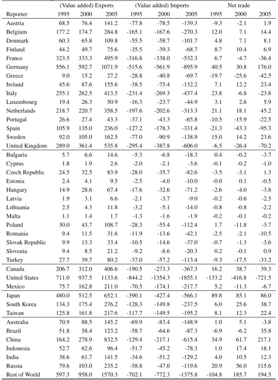
Table 1 reports the figures for exports and imports of goods and services in gross terms in billions of US dollars. As the value of a country’s exports or imports is made of all value added in the stages of production this also equals trade in value added terms. Therefore net gross trade also equals net value added trade for a country.

First, in all countries the magnitude of exports and imports increased quite strongly, particularly for countries in the EU-12 where figures are three times higher on average in 2005 compared to 1995 and in China where the exports increased by a factor of five and imports by a factor of 4.8. The last three columns present net trade figures where a negative sign implies that this country is a net importer and a positive sign that it is a net exporter. Within the EU-15 countries some countries like France and Italy became net imports and for a number of other countries the trade balance worsened (e.g. Greece, Portugal, Spain, United Kingdom). The other countries show rather stable or even increasing positive net exports, particularly so for Germany. Austria switched from a deficit to a surplus. Most of the new member states show trade deficits with trends rather mixed across countries. For example, Poland turned from slightly positive in 1995 to strongly negative in 2000 but reduced the deficit again in 2005 whereas Romania shows a worsening trade balance. Turkey also shows a worsening trade balance over time. One can also clearly see the rising trade deficit of the US which amounted to more than 700 billion US dollars in 2005 and the rapidly rising trade surplus of China. Net trade for the European countries has been or has slipped into the negative for all years and country groups. The EU-15 in particular turned a trade surplus of around 65 billion US dollars into a trade deficit of similar magnitude. The Asian countries, Japan, Korea and Taiwan, and the other countries all show a trade surplus over this period with the only exception being Australia in 2005 and Brazil. An important distinction with respect to production networks and trade in value added might be to differentiate between trade in intermediates and final goods. Let us therefore start with some stylized facts about trade in intermediates and final goods summarizing a few results on the relative importance and patterns of trade in intermediates which are the vehicle for international supply chains. We present only a short overview of some important stylized facts with respect to trade in intermediates as compared to trade in final products, however with an emphasis on the former category (see also Chen et al., 2005; Miroudot et al., 2009). This is based on detailed trade data as outlined below. A more detailed analysis for the EU countries can be found in Stehrer et al. (2010). The figures presented here are based on the data used for the construction of the WIOD database. We emphasize this as the notion of ”supply chains” - as often emphasized in case

(17)

Table 1 Trade in goods and services and trade in value added, in bn US-$

(Value added) Exports (Value added) Imports Net trade Reporter 1995 2000 2005 1995 2000 2005 1995 2000 2005 Austria 68.5 76.4 141.2 -77.8 -78.5 -139.3 -9.3 -2.1 1.9 Belgium 177.2 174.7 284.8 -165.1 -167.6 -270.3 12.0 7.1 14.4 Denmark 60.3 65.8 109.8 -55.5 -58.7 -101.7 4.8 7.1 8.1 Finland 44.2 49.7 75.6 -35.5 -39.3 -68.7 8.7 10.4 6.9 France 323.5 333.3 495.9 -316.8 -338.0 -532.3 6.7 -4.7 -36.4 Germany 556.1 592.7 1071.9 -515.6 -561.9 -895.9 40.5 30.8 176.0 Greece 9.0 15.2 27.2 -28.8 -40.8 -69.7 -19.7 -25.6 -42.5 Ireland 45.6 87.6 155.6 -38.5 -75.4 -132.2 7.1 12.2 23.4 Italy 255.1 262.5 413.5 -231.4 -269.3 -437.4 23.8 -6.8 -23.8 Luxembourg 19.4 26.3 50.9 -16.3 -23.7 -44.9 3.1 2.6 5.9 Netherlands 218.7 220.7 358.5 -197.6 -202.6 -313.3 21.1 18.1 45.2 Portugal 26.6 27.4 43.3 -37.1 -43.3 -65.8 -10.5 -15.9 -22.5 Spain 105.9 135.0 236.0 -127.2 -178.3 -331.4 -21.3 -43.3 -95.3 Sweden 92.0 105.0 162.5 -77.0 -90.9 -138.9 15.0 14.2 23.6 United Kingdom 289.0 361.4 535.8 -295.4 -387.8 -606.0 -6.5 -26.4 -70.2 Bulgaria 5.7 6.6 14.6 -5.3 -6.8 -18.3 0.4 -0.2 -3.7 Cyprus 1.8 1.9 2.6 -2.0 -2.1 -3.6 -0.1 -0.2 -1.0 Czech Republic 24.5 32.5 83.9 -28.0 -35.7 -82.6 -3.5 -3.1 1.3 Estonia 2.4 4.1 9.5 -2.5 -4.0 -10.0 -0.0 0.1 -0.5 Hungary 14.9 28.6 67.4 -17.6 -32.6 -71.2 -2.6 -4.0 -3.8 Latvia 1.9 3.1 6.6 -2.1 -3.7 -9.0 -0.2 -0.6 -2.5 Lithuania 2.5 4.3 11.8 -3.2 -5.1 -14.0 -0.8 -0.8 -2.2 Malta 1.1 1.4 1.7 -1.3 -1.6 -1.9 -0.2 -0.1 -0.2 Poland 30.0 43.7 108.7 -28.3 -55.4 -112.4 1.7 -11.8 -3.7 Romania 9.4 11.5 31.6 -11.9 -13.6 -42.1 -2.5 -2.1 -10.5 Slovak Republic 9.9 13.3 33.4 -10.5 -14.6 -37.0 -0.7 -1.3 -3.6 Slovenia 9.4 8.5 21.2 -9.2 -8.6 -20.3 0.2 -0.1 0.9 Turkey 27.7 39.7 80.2 -37.0 -57.2 -113.4 -9.3 -17.5 -33.2 Canada 206.7 312.0 406.6 -190.5 -273.3 -367.3 16.2 38.7 39.3 United States 711.0 937.5 1133.6 -844.2 -1354.3 -1855.1 -133.2 -416.8 -721.5 Mexico 75.7 162.8 211.0 -70.5 -174.1 -217.7 5.2 -11.3 -6.7 Japan 480.0 512.5 652.1 -390.1 -427.4 -566.1 89.8 85.1 86.0 South Korea 134.3 175.4 276.2 -128.3 -149.8 -237.5 6.0 25.6 38.7 Taiwan 125.8 161.8 217.6 -117.7 -149.5 -195.2 8.1 12.3 22.4 Australia 70.9 88.5 145.2 -69.9 -83.4 -148.9 1.0 5.1 -3.8 Brazil 51.8 58.4 123.2 -58.7 -64.6 -87.3 -6.9 -6.2 35.8 China 164.2 278.9 832.5 -129.4 -217.1 -615.4 34.9 61.7 217.1 Indonesia 52.7 62.6 96.4 -51.7 -45.2 -78.3 1.0 17.4 18.1 India 38.6 61.7 141.5 -34.6 -51.2 -129.2 4.0 10.5 12.3 Russia 79.6 103.0 235.2 -58.8 -47.0 -119.6 20.9 56.0 115.6 Rest of World 597.3 958.0 1570.3 -702.1 -772.3 -1375.8 -104.8 185.7 194.5

(18)

studies as mentioned above - is misleading when taking into account the fact that intermediate inputs (or components) are also themselves produced by various other inputs (intermediates and primary). Thus, though the notion of a supply chain might be relevant for particular products it does not properly account for the integrated nature of the whole production process (which might be better described as ”supply loops” or the old notion of ”roundaboutness” as discussed by B¨ohm-Bawerk (1888) for example.10 In the literature other notions are also used such as ’modular production networks’ (see e.g. Faust et al., 2004). For a discussion of supply chains and its conceptualizations see MacKechnie (2008) who proposes a discussion in terms of hierarchy, networks and markets. In essence, we point towards the fact that countries are both exporters and importers of intermediates even in narrowly defined industries which has to be taken into account when measuring trade in value added. For the sake of figuring out the value added content of a country’s exports and imports one has to notice that also intermediates exports or imports embodies value added which has to be taken into account properly. A country’s gross trade balance is resulting both from trade in final as well as trade in intermediate products.

When differentiating trade into end use categories it turns out that on average roughly fifty percent on average of total trade is traded intermediates whereas the remaining part is either for final consump-tion or gross fixed capital formaconsump-tion. Here one has to note that the category ”intermediates” is rather broad including raw materials and agricultural goods, and in particular one has to mention that it is much broader than trade in parts and components which is often considered in the literature. These patterns are relatively stable over time but can be quite heterogenous across countries. Higher shares are mostly ob-served for emerging and transition economies and resource rich economies. A second issue is that trade in intermediates seems to be concentrated in particular industries. At the lower end industries such as 16 (tobacco products), 18 (Wearing apparel), 05 (fish and fishing products), 15 (food products and bev-erages), and 19 (leather and leather products) show little trade in intermediates. Amongst the industries with the highest shares are mining industries, basic metals (27) and secondary raw materials (37) having shares of around 100 percent. Industries for which parts and components trade is important are in the middle range. These patterns are fairly consistent across countries. Finally, it is worth mentioning that also for intermediates two-way trade is important, i.e. countries import and export the same intermediates in fairly detailed product categories similar to final goods trade (see e.g. Stehrer et al., 2011).

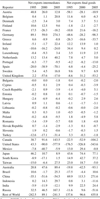
Table 2 presents the net trade figures when differentiating between these two categories from which we highlight a few interesting patterns. For example, Germany became a strong net exporter of

inter-10

One should note however that the focus in this contribution was different; see also (Samuelson, 1966) for a critical assess-ment.

(19)

Table 2 Net trade in intermediates and final goods, in bn US-$

Net exports intermediates Net exports final goods Reporter 1995 2000 2005 1995 2000 2005 Austria 48.8 26.0 12.8 -58.1 -28.1 -10.9 Belgium 0.4 1.1 20.8 11.6 6.0 -6.3 Denmark -2.5 3.4 3.0 7.4 3.7 5.1 Finland 10.6 12.5 9.6 -1.8 -2.1 -2.7 France 17.5 -26.3 -18.2 -10.8 21.6 -18.2 Germany 89.1 59.0 274.3 -48.6 -28.2 -98.3 Greece 6.6 -8.9 -8.8 -26.3 -16.6 -33.7 Ireland -5.1 -1.7 22.4 12.2 13.9 1.0 Italy -10.6 -16.2 -24.0 34.4 9.4 0.2 Luxembourg -0.4 -9.3 3.4 3.5 11.9 2.5 Netherlands 13.2 13.4 40.2 7.8 4.7 5.0 Portugal -6.3 -7.7 -9.5 -4.2 -8.2 -13.0 Spain -28.0 -38.9 -70.1 6.8 -4.4 -25.2 Sweden 5.4 4.5 16.8 9.6 9.7 6.9 United Kingdom 2.2 -57.6 -17.0 -8.6 31.2 -53.2 Bulgaria -0.0 0.0 -1.8 0.4 -0.2 -2.0 Cyprus -0.5 0.1 2.9 0.4 -0.3 -3.9 Czech Republic -2.1 0.9 -3.9 -1.4 -4.0 5.1 Estonia -0.2 0.8 1.0 0.1 -0.7 -1.5 Hungary -2.4 -6.9 -6.4 -0.2 2.9 2.6 Latvia 0.9 1.1 0.6 -1.1 -1.7 -3.1 Lithuania -0.2 -0.8 -0.2 -0.6 -0.0 -2.0 Malta 0.3 0.3 1.0 -0.5 -0.5 -1.2 Poland -0.2 -6.8 -9.5 1.8 -4.9 5.8 Romania -3.4 -3.9 -5.7 0.8 1.8 -4.8 Slovak Republic 0.7 -1.4 -2.9 -1.3 0.1 -0.7 Slovenia 1.9 0.2 -0.6 -1.7 -0.3 1.5 Turkey -12.6 -17.1 -31.4 3.3 -0.3 -1.8 Canada 38.7 91.6 143.5 -22.5 -52.9 -104.2 United States 43.3 -90.0 -377.9 -176.5 -326.8 -343.6 Mexico -7.8 -40.7 -5.9 13.0 29.4 -0.8 Japan 46.2 10.7 8.9 43.6 74.4 77.1 South Korea -8.9 -17.1 1.5 14.9 42.7 37.2 Taiwan -15.0 -6.4 27.5 23.0 18.7 -5.0 Australia 20.8 47.6 89.4 -19.8 -42.5 -93.1 Brazil 10.6 -1.7 25.3 -17.5 -4.4 10.6 China -35.1 -51.6 -54.5 69.9 113.3 271.6 Indonesia 0.2 14.3 29.7 0.8 3.1 -11.6 India -5.9 -11.9 -12.1 9.9 22.5 24.4 Russia 32.5 46.5 167.3 -11.6 9.6 -51.6 Rest of World -242.5 89.1 -241.3 137.6 96.6 435.8

(20)

mediates, whereas the trade balance with respect to final goods was always negative and even worsened. Similar dynamic patterns though at different levels might be observed for Belgium, Ireland, Luxem-bourg, Netherlands and Sweden. In other countries like Greece, Italy, Portugal, Spain and the United Kingdom both the trade balance with respect to intermediates and final goods worsened and in some cases turned from positive to negative. The remaining countries show somewhat distinct patterns. For the new member states the patterns are again rather mixed. Poland, for example, shows a negative and worsening balance in intermediates but surpluses in final goods trade, whereas Romania shows wors-ening patterns in both categories. Turkey is a strong net importer of intermediates with a small surplus in final goods trade in 1995 and 2000, which turned into negative in 2005. With respect to the NAFTA countries the US is similar to the second group above, with deteriorating negative balances in both inter-mediates (still positive in 1995) and final goods trade. Canada has a increasing surplus in interinter-mediates trade but a worsening deficit in final goods trade, whereas Mexico was net importer of intermediates and net exporter of final goods though this has changed in 2005. The Asian countries show positive net trade in both categories in most cases though with different tendencies. For example, whereas in Japan the positive trade balance in intermediates declined, it increased in final goods trade, whereas for Taiwan one can see the oppositive pattern with even switching signs. In South Korea both balances increased and even turned into positive for intermediates trade. With respect to the remaining countries Australia, Brazil, Indonesia and Russia show positive balances for intermediates trade with in most cases deficits or much lower surpluses in final goods trade though tendencies over time are rather mixed (e.g. Brazil). India and particularly China show a negative balance in intermediates trade but strong and increasing surpluses in final goods trade.

These rather mixed patterns are driven on the one hand by the countries’ endowments with natural resources (e.g. Australia, Russia) and its role in the global production process (e.g. China, Eastern European countries) and the sectoral structures. It would go beyond the scope of this paper to go into the details and determinants of these patterns, which are however important with respect to trade in value added to which we turn next.

4.2 Trade in value added

A country’s exports contain however not only domestic value added but also foreign and analogously for imports. These shares can be disentangled using the approach outlined above. In Table 3 we present the shares according to our decomposition into the five components with respect to domestic and foreign

(21)

contents of value added trade. As countries become more and more integrated in to international produc-tion processes one would expect that the share of the foreign value added content of exports would be rising over time. Further, smaller countries would be expected to show higher values. In fact, this share was rising for almost all countries as reported in the first three columns of Table 3 with a few excep-tions maybe and the magnitudes of change being rather different. For the EU-15 countries these shares range from less than 20 percent in the United Kingdom to more than 40 percent in Belgium, Ireland, and Luxembourg. There have been particularly strong increases for Eastern European countries, which show particularly high shares in most cases comparable to Taiwan , and Turkey. In the former group the shares range from 30-40 percent in most cases in 2005. For comparison, the share of Taiwan is also at 40 percent and for South Korea at 30 percent. In this country group, Japan has the lowest shares with 12 percent in 2005 which is much lower than the shares for large European countries like Germany (23 per-cent) and the UK (19 perper-cent) but in the range of the US with 13 percent in 2005 rising from 10 percent in 1995. Canada and Mexico show shares around 25 percent which are in the range of China in 2005. For this country the shares increased from 14.5 percent in 1995. The other countries tend to have lower shares ranging from less than 10 percent in Russia to about 17 percent in Indonesia, Thus, with respect to exports these results confirm the other literature of an increasing internationalization of production pointing towards the fact that smaller countries tend to have larger shares and the rapid integration of Eastern European countries. Turning to the import side, the shares of re-imports are fairly small with a mixed tendency over time. Some significant magnitudes can be found for Germany and the US. Analo-gously to the exports, we would also expect that the share of foreign imports of value added would rise as the imports from other countries increasingly embody value added from third countries. Again this is what is actually found (see three last columns in Table 3). It is interesting to note that the the shares are much more similar across countries pointing towards the fact that bilateral relations are more important. Splitting up into final goods and intermediates it turns out that the shares by use category are not too different for the individual countries though there are some notable exceptions. Particularly, the shares of the foreign multilateral content of VA imports tend to be lower for the more advanced countries. The reason for this is that these countries’ shares in bilateral content of VA imports of intermediates are high because of imports of raw materials (also from the rest of the world). Importantly however, in most cases these shares are increasing over time both for final and intermediates goods trade which implies that the production of intermediates goods trade has also become more integrated over time.11

11

(22)

Table 3 Decomposition of total value added trade (in %)

Foreign VA content Foreign VA content of exports Re-Imports of VA of multilateral imports Reporter 1995 2000 2005 1995 2000 2005 1995 2000 2005 Austria 22.1 27.0 31.1 0.8 0.9 0.7 18.7 22.9 25.3 Belgium 39.1 43.6 43.6 0.9 0.8 0.9 19.8 23.1 25.2 Denmark 24.8 29.8 32.0 0.3 0.6 0.7 22.5 23.1 24.9 Finland 21.9 26.0 28.9 0.4 0.6 0.5 17.0 21.5 23.7 France 18.2 23.1 23.0 2.0 1.7 1.8 19.0 22.2 25.1 Germany 16.0 21.4 23.1 4.0 3.9 5.2 18.5 21.6 23.9 Greece 18.2 24.3 22.3 0.1 0.1 0.2 19.4 20.1 24.0 Ireland 39.1 47.4 42.8 0.2 0.2 0.2 18.0 16.0 16.1 Italy 17.3 19.3 20.3 1.2 1.3 1.4 18.9 21.5 24.2 Luxembourg 45.3 58.5 59.8 0.1 0.1 0.1 19.7 17.2 17.4 Netherlands 31.2 34.3 34.0 1.1 1.0 1.4 16.8 18.9 21.8 Portugal 25.4 27.7 28.3 0.2 0.2 0.3 18.8 23.5 24.5 Spain 19.3 25.4 24.8 0.6 0.7 0.8 19.7 22.6 24.1 Sweden 24.8 29.3 29.9 0.7 0.6 0.7 21.8 22.3 25.4 United Kingdom 19.0 19.0 18.6 1.5 1.5 1.5 19.7 23.1 24.6 Bulgaria 29.4 36.9 42.0 0.1 0.0 0.1 17.0 21.0 26.2 Cyprus 25.0 28.4 24.0 0.0 0.0 0.0 20.8 21.2 23.0 Czech Republic 29.1 37.7 43.1 0.8 0.5 0.5 19.8 23.9 27.0 Estonia 36.2 44.0 42.8 0.1 0.1 0.1 21.3 23.8 26.1 Hungary 27.6 47.3 45.8 0.1 0.2 0.3 18.5 24.1 27.4 Latvia 25.2 27.6 31.0 0.1 0.1 0.2 22.0 25.7 29.0 Lithuania 32.2 33.1 35.0 0.1 0.1 0.2 19.0 20.6 23.3 Malta 47.1 52.3 44.0 0.0 0.0 0.0 20.7 25.1 24.4 Poland 16.1 22.3 28.9 0.2 0.3 0.4 19.8 24.8 25.9 Romania 25.0 26.6 29.5 0.0 0.1 0.1 19.4 23.4 25.4 Slovak Republic 32.1 43.8 46.2 0.7 0.3 0.3 21.4 24.3 28.4 Slovenia 30.7 34.5 38.7 0.1 0.1 0.1 22.1 26.8 30.5 Turkey 12.8 18.1 22.5 0.1 0.2 0.2 19.5 23.6 25.5 Canada 25.1 26.9 23.1 1.3 1.9 2.0 12.6 13.7 16.8 United States 9.7 11.0 13.3 6.9 8.6 6.2 13.1 14.4 17.9 Mexico 22.6 27.7 25.9 0.5 0.8 0.9 13.0 15.3 21.0 Japan 6.6 8.9 12.1 2.2 2.2 2.1 13.1 15.9 18.6 South Korea 22.7 28.6 30.5 0.5 0.6 0.8 13.6 14.2 18.4 Taiwan 31.0 34.1 40.4 0.3 0.5 0.8 12.1 14.7 17.7 Australia 11.3 12.4 12.0 0.3 0.5 0.7 15.8 17.7 22.3 Brazil 6.8 9.7 9.8 0.4 0.2 0.3 16.2 17.5 20.7 China 14.5 15.9 23.0 0.6 1.1 2.7 16.8 20.1 22.7 Indonesia 15.8 18.3 16.8 0.2 0.4 0.5 16.3 15.6 20.2 India 7.7 11.0 14.0 0.1 0.2 0.5 16.0 16.1 22.1 Russia 7.4 9.0 6.4 0.8 0.8 1.3 20.0 21.1 23.5 Rest of World 21.4 18.0 24.3 1.2 3.0 3.3 12.4 10.8 12.5

(23)

4.3 Trade in factors

Trade in value added is itself composed of trade in capital and labor as outlined above. From a theo-retical perspective the HOV results suggest that countries being abundant with labor (capital) would be net exporters of labor (capital) services at least in productivity adjusted terms. As in this paper we focus on trade in value terms (rather than in physical units) this picture becomes distorted as we allow for dif-ferences in factor rewards (i.e. no factor-price equalization).12 However, the picture is already distorted when allowing for trade in intermediates or ’trade in tasks’ (see Baldwin and Robert-Nicoud, 2010).

4.3.1 Capital and labor

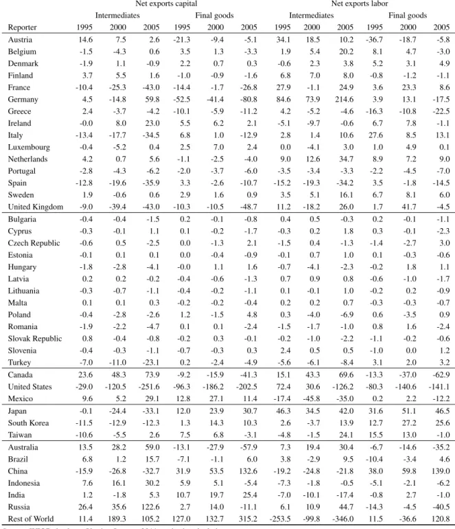
Table 4 presents the results when using capital and labor coefficients instead of value added coefficients. As the former two sum up to the latter trade flows in capital and labor must also sum up to flows in value added terms. In the EU-15 most countries with only a few exceptions (Finland, Ireland, Luxem-bourg, Sweden) are net importers of capital with the deficit rising in most cases. The reason behind is probably the rising raw material prices showing up as capital income. A number of countries how-ever are net exporters of labor and have become increasingly so: Austria, Belgium, Denmark, Germany, Netherlands, and Sweden show rising trade surpluses with respect to labor whereas for Finland, France, Italy, Luxembourg, and the UK the surplus is rather stable or fluctuates. For the other countries one can observe deficits which are rising in some cases like Greece and Spain. The Eastern European countries are almost without exception net importers of capital. With respect to labor the evidence is rather mixed. For example the Czech Republic and Slovenia show a surplus at least in 2005 whereas Hungary, Poland, Romania and Slovak Republic showing a negative balance. Turkey is both a net importer of capital and labor and increasingly so.

For the NAFTA states the evidence is again rather mixed. Canada is running a trade surplus both in labor and capital with the surplus in capital being much larger. The US is running a deficit which is increasing quite rapidly in both categories. Particularly, for capital the deficit went from positive (125.3 in 1995) to strongly negative (-454.1 in 2005); with respect to labor the US has been a net importer over the whole period but again this worsened from -7.9 in 1995 to -267.3 in 2005. Mexico was a net exporter of capital and became a net importer of labor which is somewhat surprising requires a more thorough analysis.

12

This will be undertaken in future work along the lines testing the HOV model. This paper aims at some on trade in factors in value terms.

(24)

Table 4 Net trade in capital and labor (total trade), in bn US-$ Net exports capital Net exports labor Reporter 1995 2000 2005 1995 2000 2005 Austria -6.7 -2.0 -2.5 -2.6 -0.1 4.4 Belgium 2.1 -2.9 -2.7 10.0 10.1 17.2 Denmark 0.2 1.8 -0.6 4.6 5.4 8.7 Finland 2.7 4.6 0.0 6.1 5.8 6.9 France -24.8 -26.9 -69.8 31.5 22.2 33.4 Germany -48.0 -56.2 -21.1 88.5 87.0 197.1 Greece -7.6 -9.6 -15.4 -12.1 -16.0 -27.1 Ireland 5.5 14.2 25.1 1.7 -2.0 -1.7 Italy -6.6 -16.7 -47.4 30.4 9.9 23.6 Luxembourg 2.1 1.9 2.8 1.0 0.7 3.1 Netherlands 3.1 -1.7 1.6 18.0 19.8 43.7 Portugal -4.8 -8.0 -12.2 -5.7 -7.8 -10.3 Spain -9.6 -22.2 -46.6 -11.7 -21.1 -48.7 Sweden 4.8 1.0 1.5 10.2 13.2 22.1 United Kingdom -19.3 -50.0 -91.7 12.8 23.6 21.6 Bulgaria -0.2 -0.5 -2.3 0.6 0.3 -1.4 Cyprus -0.2 -0.2 -0.6 0.0 0.0 -0.4 Czech Republic -0.6 -0.8 -0.4 -2.9 -2.4 1.7 Estonia -0.1 -0.3 -0.8 0.0 0.4 0.3 Hungary -1.8 -1.7 -2.6 -0.8 -2.3 -1.3 Latvia -0.2 -0.5 -1.6 0.0 -0.1 -0.9 Lithuania -0.7 -1.0 -2.2 -0.1 0.2 0.0 Malta -0.1 -0.1 -0.1 -0.1 -0.0 -0.1 Poland 0.8 -4.3 2.2 0.9 -7.5 -5.9 Romania -1.8 -2.0 -7.2 -0.7 -0.1 -3.4 Slovak Republic 0.6 -0.1 -0.9 -1.3 -1.2 -2.7 Slovenia -1.2 -0.7 -0.8 1.4 0.5 1.7 Turkey -6.8 -13.3 -28.0 -2.5 -4.1 -5.2 Canada 14.4 32.5 32.6 1.8 6.3 6.8 United States -125.3 -306.7 -454.1 -7.9 -110.0 -267.3 Mexico 22.4 32.3 40.5 -17.2 -43.6 -47.2 Japan 12.0 -0.5 -2.4 77.9 85.6 88.5 South Korea -10.1 1.4 -2.0 15.3 23.5 39.5 Taiwan -3.1 1.3 -0.5 10.7 11.5 23.1 Australia 0.4 0.3 1.1 0.6 4.8 -4.8 Brazil -0.3 0.2 21.7 -6.6 -6.3 14.1 China 16.0 26.7 100.0 18.8 35.1 117.2 Indonesia 13.5 21.2 24.8 -12.4 -3.9 -6.7 India 11.8 17.9 30.8 -7.8 -7.4 -18.4 Russia 29.1 49.6 111.5 -8.2 6.4 4.1 Rest of World 138.4 322.0 420.4 -242.1 -136.4 -225.2

(25)

All Asian countries have been strong net exporters of labor and increasingly so for South Korea and Taiwan and in most cases net importers of capital though the deficits are rather small. With respect to the remaining countries it turns out that these are net importers of labor in most cases with the exception of China and Russia. China shows a large and increasing surplus both for capital and labor. All countries in this group are also net exporters of capital with stronger increases of the surplus observed in Brazil, China, Indonesia, India and Russia.

Here it is important to differentiate between trade in intermediates and trade in final goods partly because trade in intermediates includes both raw materials and also high-tech components for example. We therefore show the trade balances in capital and labor differentiating between intermediates and final goods in Table 5. Let us highlight a few examples. On the one hand, countries exporting raw materials like Russia (oil), Australia (mining) and maybe Canada have increased the trade surplus in capital particularly in intermediates trade whereas the balance with respect to final goods worsened. This was similarly the case when looking at labor. On the other hand, countries like the US, UK, Italy, Japan and maybe also Turkey face larger and increasing trade deficits in intermediates with respect to capital in particular and in some cases also with respect to labor (e.g. US). China faces a large trade deficit in intermediates with respect to capital and labor with the former deteriorating over time. It however runs trade surpluses in final goods exports both with respect to capital and labor. Finally, Germany has a surplus in intermediates trade both in capital (apart from 2000) and labor, with the latter being much more important in magnitude. It runs a trade deficit in final goods trade with respect to capital but a surplus in final goods trade with respect to labor though this turned negative in 2005. A more detailed analysis of these pattern would require to look at the country specific patterns of trade with respect to the domestic and foreign contents in a bilateral way which has to be postponed to future analysis.

Table 6 presents however the components of value added trade with respect to the domestic and foreign content differentiating between capital and labor (we leave out the share of re-imports as this is rather small). Overall, these are quite similar to the ones for total trade and also the patterns across countries are quite similar. Again, the share of foreign value added content of exports tend to be larger and more disperse as compared to the share of the multilateral foreign value added content of imports. There is however no clear pattern of whether these shares are higher or lower for capital or labor across countries.

(26)

Table 5 Net trade in capital and labor by use categories, in bn US-$

Net exports capital Net exports labor

Intermediates Final goods Intermediates Final goods Reporter 1995 2000 2005 1995 2000 2005 1995 2000 2005 1995 2000 2005 Austria 14.6 7.5 2.6 -21.3 -9.4 -5.1 34.1 18.5 10.2 -36.7 -18.7 -5.8 Belgium -1.5 -4.3 0.6 3.5 1.3 -3.3 1.9 5.4 20.2 8.1 4.7 -3.0 Denmark -1.9 1.1 -0.9 2.2 0.7 0.3 -0.6 2.3 3.8 5.2 3.1 4.9 Finland 3.7 5.5 1.6 -1.0 -0.9 -1.6 6.8 7.0 8.0 -0.8 -1.2 -1.1 France -10.4 -25.3 -43.0 -14.4 -1.7 -26.8 27.9 -1.1 24.9 3.6 23.3 8.6 Germany 4.5 -14.8 59.8 -52.5 -41.4 -80.8 84.6 73.9 214.6 3.9 13.1 -17.5 Greece 2.4 -3.7 -4.2 -10.1 -5.9 -11.2 4.2 -5.2 -4.6 -16.3 -10.8 -22.5 Ireland -0.0 8.0 23.0 5.5 6.2 2.1 -5.1 -9.7 -0.6 6.7 7.8 -1.1 Italy -13.4 -17.7 -34.5 6.8 1.0 -12.9 2.8 1.4 10.6 27.6 8.5 13.1 Luxembourg -0.4 -5.2 0.4 2.5 7.0 2.4 0.0 -4.1 3.0 1.0 4.9 0.1 Netherlands 4.2 0.7 5.6 -1.1 -2.5 -4.0 9.0 12.6 34.7 8.9 7.2 9.0 Portugal -2.8 -4.3 -6.2 -2.0 -3.7 -6.0 -3.5 -3.4 -3.3 -2.2 -4.5 -7.0 Spain -12.8 -19.6 -35.9 3.3 -2.6 -10.7 -15.2 -19.3 -34.2 3.5 -1.8 -14.5 Sweden 1.9 -0.6 0.6 2.9 1.6 0.9 3.5 5.1 16.1 6.7 8.1 6.0 United Kingdom -9.0 -39.4 -43.0 -10.3 -10.5 -48.7 11.2 -18.2 26.0 1.7 41.7 -4.5 Bulgaria -0.4 -0.4 -1.5 0.2 -0.1 -0.8 0.4 0.5 -0.3 0.2 -0.1 -1.1 Cyprus -0.3 -0.1 1.1 0.1 -0.2 -1.7 -0.3 0.2 1.8 0.3 -0.1 -2.3 Czech Republic -0.6 0.5 -2.5 0.0 -1.3 2.1 -1.5 0.4 -1.3 -1.4 -2.7 3.0 Estonia -0.1 0.1 0.1 0.0 -0.4 -0.9 -0.1 0.7 1.0 0.1 -0.3 -0.6 Hungary -1.8 -2.8 -4.1 -0.0 1.1 1.6 -0.7 -4.1 -2.3 -0.2 1.8 1.1 Latvia 0.2 0.2 -0.2 -0.4 -0.6 -1.3 0.7 0.9 0.8 -0.6 -1.0 -1.7 Lithuania -0.3 -0.7 -1.1 -0.4 -0.2 -1.1 0.1 -0.1 1.0 -0.2 0.2 -0.9 Malta 0.1 0.1 0.3 -0.2 -0.2 -0.4 0.2 0.2 0.7 -0.3 -0.3 -0.7 Poland -0.4 -2.8 -2.6 1.2 -1.5 4.8 0.3 -4.0 -6.9 0.6 -3.5 0.9 Romania -1.9 -2.2 -4.7 0.1 0.1 -2.4 -1.5 -1.7 -1.0 0.8 1.6 -2.4 Slovak Republic 0.8 -0.4 -0.8 -0.2 0.3 -0.1 -0.2 -1.0 -2.2 -1.1 -0.2 -0.6 Slovenia -0.4 -0.3 -1.1 -0.7 -0.3 0.3 2.4 0.5 0.5 -1.0 0.0 1.2 Turkey -7.0 -11.0 -23.1 0.2 -2.4 -4.9 -5.6 -6.1 -8.4 3.1 2.0 3.2 Canada 23.6 48.3 73.9 -9.2 -15.9 -41.3 15.1 43.3 69.6 -13.3 -37.0 -62.9 United States -29.0 -120.5 -251.6 -96.3 -186.2 -202.5 72.4 30.6 -126.2 -80.3 -140.6 -141.1 Mexico 9.6 5.2 29.1 12.8 27.1 11.4 -17.4 -45.8 -35.0 0.2 2.2 -12.2 Japan -0.1 -24.4 -33.1 12.0 23.9 30.7 46.3 34.5 42.0 31.6 51.1 46.5 South Korea -11.5 -12.9 -12.3 1.3 14.3 10.3 2.6 -3.7 13.9 12.7 27.2 25.6 Taiwan -10.6 -5.5 2.6 7.5 6.8 -3.1 -4.8 -1.5 24.1 15.5 13.0 -1.0 Australia 13.5 28.2 59.0 -13.1 -27.9 -57.9 7.3 19.4 30.4 -6.7 -14.6 -35.2 Brazil 6.8 1.2 15.7 -7.1 -1.1 6.0 3.8 -2.9 9.5 -10.4 -3.4 4.6 China -15.9 -26.8 -32.7 31.9 53.5 132.6 -19.2 -24.8 -21.8 38.0 59.8 139.0 Indonesia 7.6 16.1 30.2 5.9 5.1 -5.4 -7.3 -1.8 -0.5 -5.1 -2.1 -6.2 India 1.2 -1.8 5.3 10.7 19.7 25.4 -7.0 -10.1 -17.4 -0.8 2.7 -1.0 Russia 26.4 35.6 122.6 2.7 14.0 -11.1 6.1 10.9 44.7 -14.3 -4.5 -40.5 Rest of World 11.4 189.3 105.2 127.0 132.7 315.2 -253.5 -99.8 -346.0 11.5 -36.6 120.8

(27)

Table 6 Decomposition of trade in factors (total trade), in %

Capital Labor

Foreign VA content Foreign VA content Foreign VA content Foreign VA content of exports of imports (multilateral) of exports of imports (multilateral) Reporter 1995 2000 2005 1995 2000 2005 1995 2000 2005 1995 2000 2005 Austria 26.1 28.6 33.3 19.2 25.4 28.4 19.9 26.1 29.7 18.4 21.3 23.1 Belgium 41.8 49.0 49.4 21.8 24.5 25.6 37.6 40.3 39.4 18.7 22.0 24.9 Denmark 27.0 31.9 36.0 24.0 24.2 26.6 23.5 28.5 29.4 21.6 22.4 23.7 Finland 23.7 26.7 33.4 17.8 22.6 23.5 20.8 25.5 25.8 16.5 20.8 23.9 France 23.2 28.1 31.0 19.7 23.2 26.6 15.9 20.4 19.1 18.5 21.5 23.9 Germany 23.0 30.0 29.9 19.2 22.5 25.3 13.1 17.4 19.4 17.9 21.0 22.8 Greece 19.6 23.0 20.4 20.5 21.2 25.6 17.4 25.4 24.4 18.7 19.4 22.9 Ireland 34.0 35.3 33.8 20.1 19.5 18.8 43.1 57.9 51.5 16.7 14.1 14.4 Italy 20.9 22.6 26.5 19.2 22.0 24.6 15.5 17.3 16.9 18.6 21.2 23.9 Luxembourg 44.9 59.8 63.9 19.2 16.5 17.1 45.6 57.2 56.1 20.0 17.8 17.6 Netherlands 33.7 39.4 40.0 18.5 19.8 22.5 29.9 31.2 30.1 15.8 18.2 21.2 Portugal 27.3 32.5 33.5 19.7 24.9 26.3 24.3 25.1 25.3 18.3 22.5 23.2 Spain 19.8 27.9 27.0 20.0 23.1 25.3 19.0 23.9 23.3 19.5 22.2 23.2 Sweden 25.2 32.6 34.9 23.4 24.4 26.8 24.5 27.4 26.9 20.7 20.9 24.3 United Kingdom 22.5 26.0 26.1 19.7 23.0 25.9 17.1 15.7 15.0 19.7 23.2 23.6 Bulgaria 37.8 48.5 51.1 14.8 19.3 27.8 23.5 28.8 35.9 19.1 22.5 24.9 Cyprus 31.4 38.0 31.4 20.9 20.9 24.2 21.5 22.7 19.6 20.8 21.5 22.2 Czech Republic 28.4 36.1 44.3 21.4 26.6 29.3 29.5 38.8 42.2 18.8 22.2 25.3 Estonia 39.5 54.6 50.6 22.2 20.8 26.9 34.2 36.9 37.9 20.7 26.7 25.5 Hungary 32.6 47.1 47.0 18.3 25.6 29.3 24.5 47.4 44.9 18.7 23.0 26.0 Latvia 30.3 34.3 39.9 22.2 27.1 31.5 22.2 23.8 25.9 21.8 24.6 27.0 Lithuania 43.9 48.6 49.1 16.8 18.4 21.3 25.1 24.2 25.5 21.1 22.8 25.4 Malta 46.7 57.4 47.6 23.1 26.6 28.9 47.3 49.1 41.9 19.4 24.0 21.6 Poland 16.7 21.9 27.1 19.9 26.9 27.0 15.6 22.5 30.5 19.8 23.4 25.0 Romania 33.1 35.8 38.2 19.5 23.5 26.2 20.9 22.0 24.6 19.3 23.2 24.7 Slovak Republic 28.1 41.9 44.2 20.9 23.7 27.2 36.3 45.6 48.2 21.7 24.7 29.5 Slovenia 46.9 42.2 45.1 23.5 28.6 33.2 25.1 30.5 34.9 21.3 25.6 28.4 Turkey 18.4 27.4 34.3 19.0 22.9 24.4 10.2 13.9 16.7 19.9 24.1 26.5 Canada 22.8 23.8 21.7 14.2 15.9 18.5 26.7 29.6 24.3 11.6 12.3 15.5 United States 12.4 15.1 16.7 12.1 13.7 17.2 8.2 8.6 10.9 14.0 15.0 18.7 Mexico 12.8 17.0 17.4 15.0 18.3 22.4 40.5 44.9 41.8 11.7 13.3 19.8 Japan 7.8 11.0 14.6 12.5 15.0 17.2 5.9 7.4 10.0 13.5 16.8 20.1 South Korea 30.8 33.7 37.4 13.4 13.5 17.9 18.7 25.2 25.8 13.8 15.0 18.9 Taiwan 37.9 37.8 47.7 13.5 16.6 19.1 27.4 31.8 35.2 11.1 13.5 16.6 Australia 12.0 14.0 12.5 14.9 16.3 20.9 10.7 11.0 11.5 16.4 18.9 23.7 Brazil 6.4 9.0 9.5 14.7 16.4 19.1 7.1 10.5 10.2 17.5 18.5 22.3 China 14.7 16.5 23.8 17.1 19.2 21.6 14.4 15.5 22.3 16.5 20.8 23.8 Indonesia 10.4 13.0 13.2 16.1 14.8 18.0 26.6 29.4 24.7 16.4 16.3 22.7 India 5.2 8.1 10.8 13.7 13.6 18.7 14.5 18.2 21.7 18.0 18.8 26.0 Russia 4.9 6.2 4.1 18.2 19.6 23.3 12.8 15.2 11.9 21.4 22.2 23.7 Rest of World 12.4 11.1 16.5 14.0 11.6 14.3 36.5 29.8 36.5 11.6 10.3 11.4

(28)

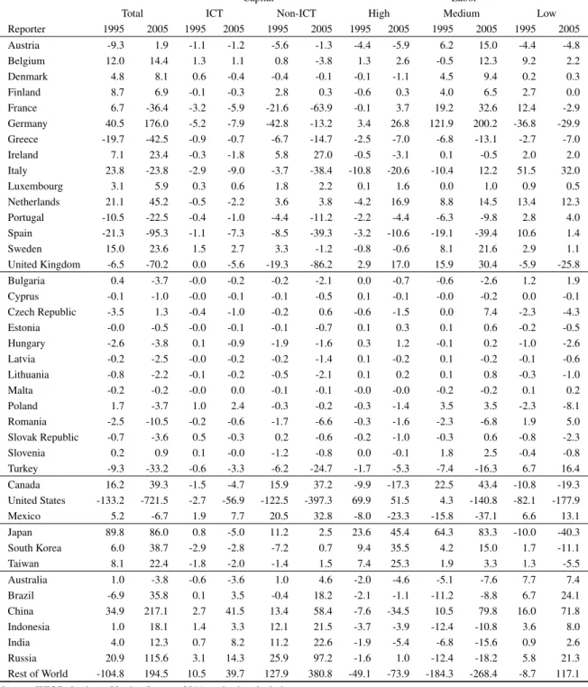
4.3.2 ICT and Non-ICT capital

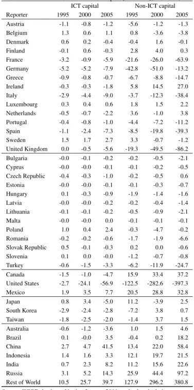
Now we move on to split up the capital component into ICT and Non-ICT capital and later on also labor into its subcomponents.13 Table 7 presents the results for the two capital categories.

First, one has to note that trade and trade balances in ICT capital are generally lower than for Non-ICT capital. In most cases, surplus countries are net exporters of both types of capital. Particularly, the US also shows a worsening trade deficit in the value of ICT capital whereas China shows a rising surplus. More generally, some advanced countries which would have been expected to be net exporters of ICT capital turn out to show a negative balance and vice versa for the less developed countries. Thus this deserves some more detailed explanations with respect to trade structures, factor rewards, and so on.

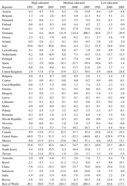
4.3.3 Educational attainment categories

Finally, we present in Table 8 the results when splitting up trade flows in labor terms into the components high-educated and medium and low educated.

With respect to high educated labor the pattern is mostly as expected: the more advanced countries and those better endowed with skilled labor are also net exporters of it. This is the case for most of the EU-15 countries, the notable exceptions are Austria and Italy whereas other countries with deficits like Greece, Portugal and Spain are less well endowed with skilled labor. Also the US is showing a trade surplus with respect to skilled labor which is however slightly declining over time. The other two countries (Canada and Mexico) run larger deficits. The Asian countries also show surpluses with respect to skilled labor which are rising in all cases. All the other have experienced deficits; particularly, China shows a rising deficit in the trade of skilled labor. Regarding medium educated employment, most of the EU-15 countries show trade surpluses as expected with the exceptions of Greece, Spain and Portugal. These surpluses are rather high and/or increasing in Austria, Germany, Netherlands, Sweden and the UK. Also the Eastern European countries show in a number of cases a surplus in this category with the exceptions of Bulgaria and Romania. Significant and rising surpluses are found in the Czech Republic, Poland and Slovenia. The US started with a surplus in this category of medium skilled workers but was switching to a deficit in 2000 which was then further increasing. Canada is running a surplus whereas Mexico shows a deteriorating deficit. Again the Asian countries show increasing surpluses which is however rather small in the case of Taiwan. Within the group of the remaining countries all

13

Data for ICT shares in capital income are preliminary and based on imputed values for some countries; thus results will be revised and to be interpreted cautiously.

(29)

Table 7 Net trade in ICT and Non-ICT capital (total trade), in bn US-$ ICT capital Non-ICT capital Reporter 1995 2000 2005 1995 2000 2005 Austria -1.1 -0.8 -1.2 -5.6 -1.2 -1.3 Belgium 1.3 0.6 1.1 0.8 -3.6 -3.8 Denmark 0.6 0.2 -0.4 -0.4 1.6 -0.1 Finland -0.1 0.6 -0.3 2.8 4.0 0.3 France -3.2 -0.9 -5.9 -21.6 -26.0 -63.9 Germany -5.2 -5.2 -7.9 -42.8 -51.0 -13.2 Greece -0.9 -0.8 -0.7 -6.7 -8.8 -14.7 Ireland -0.3 -0.3 -1.8 5.8 14.5 27.0 Italy -2.9 -4.4 -9.0 -3.7 -12.3 -38.4 Luxembourg 0.3 0.4 0.6 1.8 1.5 2.2 Netherlands -0.5 -0.7 -2.2 3.6 -1.0 3.8 Portugal -0.4 -0.8 -1.0 -4.4 -7.2 -11.2 Spain -1.1 -2.4 -7.3 -8.5 -19.8 -39.3 Sweden 1.5 1.7 2.7 3.3 -0.7 -1.2 United Kingdom 0.0 -0.5 -5.6 -19.3 -49.5 -86.2 Bulgaria -0.0 -0.1 -0.2 -0.2 -0.5 -2.1 Cyprus -0.0 -0.0 -0.1 -0.1 -0.2 -0.5 Czech Republic -0.4 -0.3 -1.0 -0.2 -0.5 0.6 Estonia -0.0 -0.0 -0.1 -0.1 -0.3 -0.7 Hungary 0.1 -0.3 -0.9 -1.9 -1.4 -1.6 Latvia -0.0 -0.0 -0.2 -0.2 -0.4 -1.4 Lithuania -0.1 -0.1 -0.2 -0.5 -0.9 -2.1 Malta -0.0 -0.0 0.0 -0.1 -0.1 -0.1 Poland 1.0 0.4 2.4 -0.3 -4.7 -0.2 Romania -0.2 -0.2 -0.6 -1.7 -1.9 -6.6 Slovak Republic 0.5 -0.1 -0.3 0.2 0.0 -0.6 Slovenia 0.1 0.0 -0.0 -1.2 -0.7 -0.8 Turkey -0.6 -1.5 -3.3 -6.2 -11.9 -24.7 Canada -1.5 -1.0 -4.7 15.9 33.4 37.2 United States -2.7 -24.1 -56.9 -122.5 -282.6 -397.3 Mexico 1.9 3.5 7.7 20.5 28.8 32.8 Japan 0.8 3.4 -5.0 11.2 -3.9 2.5 South Korea -2.9 -2.4 -2.8 -7.2 3.8 0.7 Taiwan -1.8 -2.5 -2.0 -1.4 3.7 1.5 Australia -0.6 -1.2 -3.6 1.0 1.5 4.6 Brazil 0.1 -0.0 3.5 -0.4 0.2 18.2 China 2.7 4.7 41.5 13.4 22.0 58.4 Indonesia 1.4 1.6 3.3 12.1 19.7 21.5 India 0.7 2.3 8.2 11.2 15.6 22.6 Russia 3.1 5.2 14.3 25.9 44.4 97.2 Rest of World 10.5 25.7 39.7 127.9 296.2 380.8

(30)

Table 8 Net trade in labor by educational categories, in bn US-$

High educated Medium educated Low educated Reporter 1995 2000 2005 1995 2000 2005 1995 2000 2005 Austria -4.4 -4.3 -5.9 6.2 7.0 15.0 -4.4 -2.9 -4.8 Belgium 1.3 1.0 2.6 -0.5 4.0 12.3 9.2 5.1 2.2 Denmark -0.1 -0.0 -1.1 4.5 5.5 9.4 0.2 -0.1 0.3 Finland -0.6 -0.1 0.3 4.0 4.4 6.5 2.7 1.5 0.0 France -0.1 1.6 3.7 19.2 17.9 32.6 12.4 2.7 -2.9 Germany 3.4 0.4 26.8 121.9 114.4 200.2 -36.8 -27.7 -29.9 Greece -2.5 -4.2 -7.0 -6.8 -8.2 -13.1 -2.7 -3.6 -7.0 Ireland -0.5 -2.6 -3.1 0.1 -0.4 -0.5 2.0 1.0 2.0 Italy -10.8 -10.5 -20.6 -10.4 -4.4 12.2 51.5 24.8 32.0 Luxembourg 0.1 0.0 1.6 0.0 0.7 1.0 0.9 0.0 0.5 Netherlands -4.2 0.8 16.9 8.8 7.4 14.5 13.4 11.7 12.3 Portugal -2.2 -3.1 -4.4 -6.3 -7.4 -9.8 2.8 2.7 4.0 Spain -3.2 -3.9 -10.6 -19.1 -23.7 -39.4 10.6 6.5 1.4 Sweden -0.8 -2.0 -0.6 8.1 13.5 21.6 2.9 1.7 1.1 United Kingdom 2.9 17.8 17.0 15.9 22.3 30.4 -5.9 -16.6 -25.8 Bulgaria 0.0 -0.2 -0.7 -0.6 -0.9 -2.6 1.2 1.4 1.9 Cyprus 0.1 0.0 -0.1 -0.0 0.0 -0.2 0.0 0.0 -0.1 Czech Republic -0.6 -1.3 -1.5 0.0 1.2 7.4 -2.3 -2.3 -4.3 Estonia 0.1 0.2 0.3 0.1 0.5 0.6 -0.2 -0.2 -0.5 Hungary 0.3 0.0 1.2 -0.1 -0.9 0.2 -1.0 -1.5 -2.6 Latvia 0.1 0.1 -0.2 0.1 0.1 -0.2 -0.1 -0.2 -0.6 Lithuania 0.1 0.1 0.2 0.1 0.5 0.8 -0.3 -0.4 -1.0 Malta -0.0 -0.0 -0.0 -0.2 -0.2 -0.2 0.1 0.2 0.2 Poland -0.3 -2.5 -1.4 3.5 -0.3 3.5 -2.3 -4.7 -8.1 Romania -0.3 -0.5 -1.6 -2.3 -2.2 -6.8 1.9 2.5 5.0 Slovak Republic -0.2 -0.4 -1.0 -0.3 0.1 0.6 -0.8 -1.0 -2.3 Slovenia 0.0 -0.0 -0.1 1.8 1.0 2.5 -0.4 -0.4 -0.8 Turkey -1.7 -3.4 -5.3 -7.4 -10.1 -16.3 6.7 9.4 16.4 Canada -9.9 -13.0 -17.3 22.5 31.7 43.4 -10.8 -12.4 -19.3 United States 69.9 72.1 51.5 4.3 -52.2 -140.8 -82.1 -129.9 -177.9 Mexico -8.0 -21.9 -23.3 -15.8 -36.2 -37.1 6.6 14.5 13.1 Japan 23.6 33.7 45.4 64.3 74.7 83.3 -10.0 -22.7 -40.3 South Korea 9.4 15.8 35.5 4.2 10.4 15.0 1.7 -2.7 -11.1 Taiwan 7.4 11.4 25.3 1.9 2.0 3.3 1.3 -1.9 -5.5 Australia -2.0 -0.9 -4.6 -5.1 -2.8 -7.6 7.7 8.4 7.4 Brazil -2.1 -4.7 -1.1 -11.2 -11.2 -8.8 6.7 9.6 24.1 China -7.6 -12.2 -34.5 10.5 23.7 79.8 16.0 23.6 71.8 Indonesia -3.7 -2.9 -3.9 -12.4 -6.6 -10.8 3.6 5.5 8.0 India -1.9 -2.6 -5.4 -6.8 -7.0 -15.6 0.9 2.2 2.6 Russia -1.6 0.1 1.0 -12.4 -6.3 -18.2 5.8 12.6 21.3 Rest of World -49.1 -58.0 -73.9 -184.3 -162.0 -268.4 -8.7 83.6 117.1