University of Vermont
ScholarWorks @ UVM
Graduate College Dissertations and Theses Dissertations and Theses
2018
Novelty Detection Of Machinery Using A
Non-Parametric Machine Learning Approach
Enrique Angola University of Vermont
Follow this and additional works at:https://scholarworks.uvm.edu/graddis
Part of theComputer Sciences Commons,Mathematics Commons, and theMechanical Engineering Commons
This Thesis is brought to you for free and open access by the Dissertations and Theses at ScholarWorks @ UVM. It has been accepted for inclusion in Graduate College Dissertations and Theses by an authorized administrator of ScholarWorks @ UVM. For more information, please contact
Recommended Citation
Angola, Enrique, "Novelty Detection Of Machinery Using A Non-Parametric Machine Learning Approach" (2018).Graduate College Dissertations and Theses. 923.
NOVELTY DETECTION OF MACHINERY USING A NON-PARAMETRIC MACHINE LEARNING APPROACH
A Thesis Presented
by
Enrique D. Angola Abreu to
The Faculty of the Graduate College of
The University of Vermont
In Partial Fulfillment of the Requirements for the Degree of Master of Science Specializing in Mechanical Engineering
October, 2018
Defense Date: May 25, 2018 Thesis Examination Committee: Dryver Huston, Ph.D., Advisor Donna Rizzo, Ph.D., Chairperson Yves Dubief, Ph.D. Cynthia J. Forehand, Ph.D., Dean of the Graduate College
ABSTRACT
A novelty detection algorithm inspired by human audio pattern recognition is conceptualized and experimentally tested. This anomaly detection technique can be used to monitor the health of a machine or could also be coupled with a current state of the art system to enhance its fault detection capabilities. Time-domain data obtained from a microphone is processed by applying a short-time FFT, which returns time-frequency patterns. Such patterns are fed to a machine learning algorithm, which is designed to detect novel signals and identify windows in the frequency domain where such novelties occur. The algorithm presented in this paper uses one-dimensional kernel density estimation for different frequency bins. This process eliminates the need for data dimension reduction algorithms. The method of “pseudo-likelihood cross validation” is used to find an independent optimal kernel bandwidth for each frequency bin. Metrics such as the “Individual Node Relative Difference” and “Total Novelty Score” are presented in this work, and used to assess the degree of novelty of a new signal. Experimental datasets containing synthetic and real novelties are used to illustrate and test the novelty detection algorithm. Novelties are successfully detected in all experiments. The presented novelty detection technique could greatly enhance the performance of current state-of-the art condition monitoring systems, or could also be used as a stand-alone system.
TABLE OF CONTENTS Page LIST OF TABLES ... iv LIST OF FIGURES ... v CHAPTER 1: INTRODUCTION ... 1 1.1. General Background ... 1
1.2. A Novelty Detector Inspired By Human Audio Pattern Recognition ... 3
1.2. Translating Novelty into Mechanical Failure ... 8
1.3. Current State of the Art Condition Monitoring Systems ... 12
1.4. Motivation for a New Approach ... 13
CHAPTER 2: THEORETICAL BACKGROUND ... 15
2.1. Statistical Novelty Detection ... 15
2.2. Short-Time FFT ... 16
CHAPTER 3: BUILDING AND TESTING THE NOVELTY DETECTOR ... 19
3.1. Experimental Setup ... 19
3.2. Case Study: Illustrative Example... 20
3.3. Experimental Example 1: Conceptual Testing ... 26
3.4. Experimental Example 2: Testing and Validating the Novelty Detector ... 29
LIST OF TABLES
Table Page
Table 1: Normal test samples ... 38
Table 2: Friction between metal components – barely audible ... 39
Table 3: Increased friction between metal components ... 39
Table 4: External novelty source – highly audible ... 40
Table 5: Normal test samples with T = 20 seconds training ... 41
LIST OF FIGURES
Figure Page
Figure 1: Time frequency pattern ... 4
Figure 2: A Shewhart control chart ... 8
Figure 3: Test bench... 20
Figure 4: Original signal in time domain ... 21
Figure 5: Novelty signal in time domain ... 21
Figure 6: Time-frequency pattern with novelty ... 22
Figure 7: Original signal at bin = 40 after short-time FFT ... 23
Figure 8: Novelty signal at bin = 40 after short-time FFT ... 23
Figure 9: Original signal at bin = 80 after short-time FFT ... 24
Figure 10: Novelty signal at bin = 80 after short-time FFT ... 24
Figure 11: Results from the novelty detector ... 25
Figure 12: Fully trained novelty detector with normal signal results ... 28
Figure 13: Fully trained novelty detector with novelty results ... 28
Figure 14: Bandwidth parameter estimation ... 30
Figure 15: Overfitting example ... 32
Figure 16: PDF with bandwidth after cross-validation ... 33
CHAPTER 1: INTRODUCTION 1.1. General Background
According to Desforges [1], condition monitoring systems can be broken down into 3 different approaches:
1) Case-based reasoning
2) Model-based diagnosis
3) Non-parametric modeling
Case-based reasoning relies on imposed rules, and requires the knowledge and influence of an expert to monitor the machine. Model-based diagnosis requires an often complex, mathematical model of the system. Oftentimes a mathematical model of such complexity might be impossible to achieve in reality [1]. Non-parametric techniques approach the problem by modeling the system based on learned patterns from training data. A non-parametric model can be created by the use of neural networks [2] or statistical techniques such as Parzen Windows [3] [4] [1] [5]. Such a model can be completely automated, and does not require expert knowledge [1]. A usual drawback of non-parametric modeling is that a large number of data is required to train the model [1]. With Parzen Windows, the amount of training data needed grows exponentially relative to the dimension of the feature space. This is commonly referred to as “the curse of dimensionality” [4]. In machine learning, novelty detection can be defined as the capability to detect unknown features from data which are not part of a training set. The concept of novelty detection can be directly applied to condition monitoring systems of machinery by relating a novel sample to a possible machinery fault. Desforges performed
extensive work on novelty detection of machinery using wavelet coefficients from vibration signals and Parzen Windows as a novelty detector [1].
Due to the large dimension of the feature space of the training data, Desforges applied dimension reduction techniques to process the feature vectors, or simply collected more data [1]. It is clear that the curse of dimensionality increases the computational expense of a non-parametric novelty detector, as well as potentially causing loss of important information from the data. The model presented in this paper offers an approach where the feature space of the training vectors is simply one-dimensional, eliminating constraints originating from the curse of dimensionality.
There has also been recent research for audio novelty detectors using deep learning techniques. Marchi, et al. [6] successfully used autoencoders to build a highly accurate audio novelty detector. Said novelty detector used audio signals that were processed through a short-time-FFT followed by calculating the Mel frequency coefficients. The Mel frequency coefficients are defined as the coefficients that together form the Mel frequency cepstrum. The Mel frequency cepstrum is a form a non-linear cepstrum used to process audio signals, and it has successfully been applied to speech recognition tasks [7]. The autoencoders were able to encode the processed signal and identify novelties by decoding new signals through the trained autoencoders. It is important to note that Marchi, et al. [6] research was not done for condition monitoring systems purposes, but it could be adapted for such a purpose. A usual drawback of using deep learning techniques for machine learning tasks is that they tend to require very large amounts of data and high computational power, with the benefit of learning features from the data automatically.
1.2. A Novelty Detector Inspired By Human Audio Pattern Recognition
Inspired by the functionality of human audio pattern recognition, the goal is to create a computer model capable of learning the transient sound signature of rotating machinery. The model should recognize and alert a human when an anomaly is detected in the sound pattern. The model should also be able to identify a window in the frequency domain where such novelty occurs. The resolution of such frequency window depends on the time domain resolution in compliance with Heisenberg's uncertainty principle [8]. In the case of human audio pattern recognition, we can simplify such model by dividing it in three functional items:
1) Raw audio - sound waves: compressions and rarefactions in air
molecules due to the vibrational energy transmitted by components of the machine.
2) The human ear: processes the raw audio data and sends frequency time
dependent information to the brain.
3) The human brain: responsible for processing the information provided
by the ear; learns and stores the sound signature of the rotating machinery. A computational concept of such model can be broken down as follows:
1) Raw audio - sound waves
2) A microphone: a device responsible for transforming the compressions
and rarefactions in air molecules into digital time-domain audio data, so that it can be processed by a digital computer.
3) A digital computer: responsible for processing the raw digital audio data. A computer program to process such signal is composed of:
• Data pre-processing algorithm: an algorithm designed to convert the time-domain signal into a frequency time dependent pattern, imitating the signal produced by the human ear [9].
• Machine learning algorithm: similar to the brain; an algorithm designed
to process the information provided by the data pre-processing algorithm. This algorithm is responsible for learning the sound signature of the machinery, and should be capable of identifying anomalies.
For the data pre-processing algorithm, a short windowed Fast-Fourier-Transform (short-time FFT) is applied. The algorithm transforms the domain signal into a time-frequency domain pattern (Figure 1). Time and time-frequency resolution are fixed, and set by the choice of the window's width in time [8]. For the human ear, frequency and time resolutions are not fixed; time resolution is higher at high frequencies and lower at low frequencies, and vice versa, frequency resolution is higher at low frequencies and lower at high frequencies [9]. However, for novelty detection purposes, a time-frequency
pattern with fixed time and frequency resolution is not necessarily an impediment. It was found in experiments performed for this research that short-time FFT performs well enough for novelty detection purposes. If the goal is to ultimately approach the exact functionality of human hearing, other methods for obtaining a time-frequency domain pattern with similar time-frequency resolutions to the human ear, such as the discrete wavelet transform, could be explored [10].
A probabilistic model can be conceptualized as follows. A “monitoring node” is assigned to each frequency bin in the time-frequency domain. The function of each “monitoring node” is to statistically model the probability density function of the time-domain pattern for each frequency bin. This is achieved by using a non-parametric, adaptive, statistical approach. In other words, a Parzen Window is assigned to each frequency bin. For novelty detection purposes, each node works in parallel. In relation to human audio pattern recognition, one can think of these nodes as similar to the hair filaments in the inner ear, sending time-frequency information signals to the brain [9]. Individual nodes respond to stimuli only in a restricted region of auditory field. To build the novelty detector, the previously described model must be trained.
Training is done in three steps as follows:
1) To train the nodes, an audio sample of time = T from the machinery in “healthy” status is collected and used as a base signal. A Parzen Window is assigned to each node j. Which is used to estimate the total log-likelihood of the test pattern under the model of the training data [11]. The training sample can also be built from a pool of “healthy” data samples. The idea is to randomly pick m samples of time = T from the pool and then retrieve a random
sub-sample of time T’ = T/m from each m. Then all the subsamples are concatenated to create a training sample of time = T. This form of sampling from the data creates a more statistically significant training sample and avoids overfitting.
2) Each node must then learn the optimal bandwidth for proper probability density function estimation. There are many different techniques to estimate the optimal bandwidth [12] [13]. Pseudo log-likelihood cross-validation was used to find optimal bandwidths in experiments performed for this research. 3) To establish an individual novelty threshold for each node, Xi audio samples
(thresholding set) from the healthy rotating machinery are collected, where i is the sample number. For each data sample in the thresholding set, the log-likelihood Yij for each node is estimated from the trained Parzen Windows.
The threshold t for each j is found by setting an outlier limit using the following Z – score equation [14].
𝑡𝑗 = 𝜇𝑗± z ∗ σj
Where µj is the mean of the given set {Y1j,Y2j,...Ynj}, σj the standard deviation of
the set, and z is a constant; usually 3.
Hypothesis testing is performed individually per node to identify if a new pattern is novel. The null-hypothesis is identified as the new pattern being sampled from the learned distribution. If the null-hypothesis is rejected, then the new pattern is not sampled from the learned distribution. Therefore, it is a novel pattern. The trained nodes monitor new signals coming from the machine and calculate the total log-likelihood for each frequency bin of the new signal on the learned model. Each node activates if the novelty
threshold is exceeded and the null-hypothesis is rejected. Even though each node is working separately, networking is a potential possibility. Sharing of information between the nodes can happen as follows:
4) Due to harmonics or different phenomena by which the fault mode releases
energy, most mechanical faults will provide novelty information in more than one frequency bin. Therefore, information from more than a single node should be used to raise an alarm.
5) Communication between the nodes could transform the novelty detector into a classifier (probabilistic neural network [15] [4]), which could be useful to avoid false alarms due to novelties such as rain or noise from nearby mechanical devices that cycle on and off (fans). Classification could also be used to potentially allow the network to recognize different fault modes. A machine can also operate in different modes, and an individual novelty detector should be assigned to each mode. It is important to note that random novelties could occur from time to time, and they will not necessarily represent a mechanical failure. Monitoring should be performed over time, and an alarm should be raised only if a novelty persists over time; permanently changing the sound signature of the machine.
Chapter 3 in this thesis presents three experiments performed to build and validate this concept. The first experiment consists on evaluating step training 1 of the novelty detector by using real data for training the algorithm and synthetic data to test for novelty detection. This experiment illustrates the architecture of the novelty detector and how kernel density estimation is used as the statistical learning algorithm method to model the distribution of the machine’s sound signature. The second experiment evaluates the
algorithm on real test data and serves as a proof of concept; showing threshold calculation for hypothesis testing. The third and last experiment was designed to finally validate the algorithm, and study the novelty detector’s performance in a noisy environment. All training steps were performed as presented in this section, and a much larger and representative data set was collected.
Results from this experiment show the importance of optimal bandwidth parameter estimation, and the behavior of the novelty detector over time.
1.2. Translating Novelty into Mechanical Failure
It is of great challenge to conclude if a mechanical fault is present due to a statistical novelty detected by the algorithm. In statistical novelty detection when the null hypothesis is rejected we can affirm that a novel pattern has been found. In our particular fault detection problem a statistical novelty does not necessarily mean that a machine’s sound signature has permanently changed.
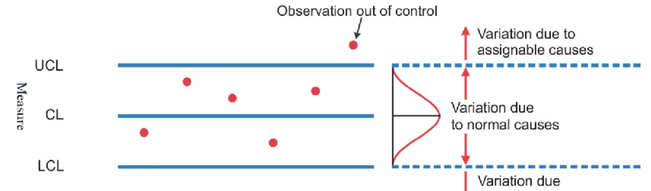
In the early 1900’s Walter Shewhart introduced the concept of control charts for statistical control. A control chart is a statistical graphical tool that illustrates the variability of a measure and identifies special-cause variations in the data, which Shewhart referred to as “assignable cause” [14]. On a control chart a control upper limit
and a lower control limit are defined, and if a sample falls outside any of these regions, it is deemed to be an “observation out of control” and must have an assignable cause according to Shewhart.
This concept can be directly applied to the novelty detection problem studied in this thesis. For this particular case the measured metric would be the log(likelihood) estimated by the parzen windows for each individual node. The upper and lower control limits are calculated with the Z-score equation presented in the last step of training for the novelty detection algorithm, which we call the novelty threshold. Following Shewhart’s theory, when a new sample falls outside of the learned threshold the variation must be due to assignable causes. The challenge for the problem studied in this thesis is to find the assignable cause for the novel sample.
Our main interest is to assign the cause either to a mechanical fault of the machine being monitored, or to a benign external factor. Firstly, the measure being monitored by the novelty detection algorithm is a likelihood estimate of the new sample based on the base signal’s probability density function, which is learned by kernel density estimation. This can provide a great deal of information from which we can estimate a metric that measures the degree of novelty of the novel sample. Secondly, the second law of thermodynamics states that the total entropy of an isolated system can never decrease over time. If the novel sample’s assignable cause is concluded to be a mechanical fault, and a new sample node outputs return to the normal region; between the upper and lower control limits; the second law of thermodynamics would be violated. Therefore, the assignable cause in this case must be concluded to be a benign novelty which is
non-related to a permanent change of the machine’s sound signature. This conclusion should be sufficient for the purposes of the novelty detection algorithm.
Many “benign” effects such as rain, thunder, a truck passing by, etc. can trigger a novelty as long as such a pattern is not part of the training set, even though they might not be directly correlated to the machine being monitored. Machines also tend to operate in very noisy environments where novel events are common. For chapter 3, section 3, it was decided to perform experiments in a noisy environment, particularly a machine shop. This was done in order to capture false alarms. The amount of novel nodes and their reported values indicate how different the new pattern is from the base signal. Monitoring the novelty over time would be of crucial necessity. If a novelty keeps appearing over time, or results keep getting further from the base signal, it would be clear that the machine's sound signature has permanently changed. Otherwise, if the signal goes back to normal and the novelty does not occur again, it is very likely that the captured novelty has no direct correlation to a permanent change in the machine’s sound signature, but rather a novelty caused by an external “benign” factor.
Establishing a degree of novelty can provide a greater insight into the practical problem of detecting a machine’s fault rather than simply stablishing if a new sample is novel or not. A high degree of novelty conveys that it is extremely likely that the new sound pattern is sampled from a completely different distribution. This could potentially mean that the sound signature of the machine has permanently changed, as long as new sound patterns keep showing high degrees of novelty. Therefore, the following are necessary to estimate if a novelty is related to the machine being monitored:
2) When a novelty reaches a high degree of novelty, this must be monitored through time. If new audio signals keep showing a high degree of novelty, it can be assumed that there is a very high chance that the machine being monitored has permanently changed.
In this thesis a lot of attention has been put to establish a metric that would let the algorithm monitor the degree of novelty for new patterns. For that we define the
Individual Node Relative Difference (INRD) and the Total Novelty Score (TNS). Given a
node in a new pattern that has raised a novelty by reporting likelihoods outside the learned threshold; rejecting the null hypothesis. The INRD is simply the relative difference between the novel likelihood and the threshold and it is calculated as follows:
𝑰𝑵𝑹𝑫𝒋 = 𝝓𝒋− 𝒕𝒋
𝒕𝒋 (1)
Where ϕis the likelihood obtained from the novelty detector for node j from the test pattern, and t is the novelty threshold for node j.
The INRD essentially normalizes the threshold and computes the distance from
novelty to normalized threshold. Storing and monitoring these values can be impractical for novelty detectors with many nodes. The TNS is a windowed sum over the INRD values, which is calculated to store more compact results. The TNS is introduced:
𝑻𝑵𝑺𝒊 = ∑ 𝑰𝑵𝑹𝑫𝒌 𝒌=𝒋+𝑵
𝒌= 𝒋
(2)
Where N is the choice if window size, j is the node number, and i is the index for the TNS for a particular chunk of nodes. For example, for a novelty detector with 220 nodes, choosing N = 10 would calculate a total of 22 Total Novelty Scores each one
representing 10 frequency bins. This concept for calculating the degree of novelty is studied in the results obtained for chapter 3, section 3.
1.3. Current State of the Art Condition Monitoring Systems
Vibration monitoring systems are very common and set the current industry standard for predictive maintenance of rotating machinery. Accelerometers are used to monitor vibration signals with the aid of state of the art digital signal processing algorithms [16].
Accelerometers are often placed near elements of interest; components that need monitoring. A tachometer is also generally used to correlate the rotational speed of the machine with the vibration signal. Raw vibration time-domain signals are generally transformed through different digital signal processing algorithms in order to easily extract features that provide critical information regarding the state of a certain component of the machine.
These features are called Condition Indicators and are of deterministic nature. For example, to monitor for shaft related faults such as misalignment or imbalance, the “shaft orders” condition indicators are often used. Shaft orders are simply the energy represented by the rotational frequency of the shaft and its harmonics. Shaft orders are often monitored through spectral analysis, which consists of performing a Fast Fourier Transform on the signal, and monitoring the peaks at the rotational frequency of the shaft and its harmonics. Sometimes, a TSA (Time Synchronous Average) is performed to pre-process the raw signal, and filter out non-synchronous signals [17]. In this particular case, the tachometer is necessary to know what the rotational frequency of the shaft is in real time [16].
Similarly, condition indicators can also be derived to detect bearing faults, gear faults, etc… These are all deterministically calculated, and are most often periodic signals. These condition indicators can be monitored by an expert, or by hypothesis testing statistical algorithms. HI (Health Indicator) is a common name used for a scalar derived from a CI monitoring statistical hypothesis testing technique [16].
The deterministic nature of current state of the art condition monitoring techniques can sometimes lead to missing obvious catastrophic faults. Pranet [16] could not detect a ball bearing fault in his experiments because the condition indicator for such a fault was designed to monitor a periodic signal coming from an impact in the inner race or outer race of the bearing. The signal being monitored did not show in his experiment, and the deterministic algorithm failed to detect the fault.
This is a clear example of how current state of the art condition monitoring does not provide sufficient predictive maintenance coverage.
1.4. Motivation for a New Approach
In this research an entirely different approach for predictive maintenance is proposed. Statistical learning theory is used to construct an unsupervised machine learning algorithm designed to by-pass the feature selection process, and detect faults such as the bearing fault missed by Pranet’s experiments [16].
Statistical learning theory is not an entirely new approach to condition monitoring of machinery. There has been previous research that has shown success for detecting machinery faults using accelerometers and machine learning algorithms [1]. However, these techniques are often shadowed by the numerous amount of research and industrial applications of current state of the art deterministic condition monitoring techniques.
There is also very little research on audio condition monitoring systems. The transient and complex nature of audio signals make it a difficult candidate for the previously discussed deterministic models. However, audio condition monitoring is a perfect candidate for machine learning algorithms, since they possess the flexibility to learn highly complex patterns from the feature space.
The intent of this research is not to compare and benchmark audio based machine learning monitoring systems against current state of the art vibration monitoring. But rather to encourage further research into both; machine learning condition monitoring and audio condition monitoring for machinery.
The predictive maintenance industry can greatly benefit from the latest advances in machine learning and current state of the art audio processing technology.
By principle, deterministic models cannot take into consideration all possible faults. Unsupervised machine learning predictive models adapt to the problem and have the flexibility to learn more complex patterns from the feature space, with the tradeoff of less interpretability. Unsupervised learning models such as the one presented in this work can be used in conjunction with industrial state-of-the art deterministic models to enhance flexibility of condition monitoring systems.
CHAPTER 2: THEORETICAL BACKGROUND 2.1. Statistical Novelty Detection
In machine learning, novelty detection can be defined as the capability to detect unknown observations from data which are not part of a training set. Novelty detection can be very useful in mechanical applications where abnormal behavior of machinery could be a symptom of a mechanical failure. Other useful applications for novelty detectors are: hand written digit recognition, radar target detection, detection of masses in mammograms, e-commerce, and statistical process control [3]. Statistical novelty detection approaches are based on building a statistical model from a set of training data and estimating if a test sample belongs to the same distribution or not [3].
There are two basic models to follow when designing a statistical novelty detector; parametric and non-parametric. Parametric methods assume that the data come from a family of known distributions. Non-parametric methods, on the other hand, do not make assumptions about the data distribution, and instead rely on estimating a distribution based on the data itself. Non-parametric methods tend to be very powerful for problems that require adaptability, and those where the underlying distribution is naturally unknown. However, non-parametric methods tend to be more computationally expensive than parametric techniques [3]. Markou [3] mentions a few robust parametric techniques that can be used for novelty detection: Probabilistic/GMM approaches (semi-parametric according to Yeung [5]) and Hidden Markov Models.
Yeung [5] argues that parametric techniques are “inappropriate” for real novelty detection problems, since the simple parametric distribution models fail to approach real
data distributions. Markou [3] also mentions a few non-parametric techniques for novelty detection: kNN based approaches, Parzen Windows, string matching approaches, and clustering approches.
2.2. Short-Time FFT
When the human auditory system listens to rotating machinery, such as a running automobile, the auditory system detects frequency variations in time. This is due to the non-stationary nature of audio signals. Sound-waves are composed of packets of close frequencies rather than pure tones [8]. The Windowed Fourier Transform offers the capability of local time-frequency decomposition, which retrieves instantaneous packets of frequencies from sound when applied to the time-domain signal. The short-time Fourier Transform for a signal f is defined by the following equation:
𝑺𝒇(𝒖, 𝝃) = ∫ 𝒇(𝒕)𝒈(𝒕 − 𝒖)𝒆∞ −𝒊𝝃𝒕𝒅𝒕
−∞ (3)
Where g(t) is a real and symmetric window, translated by u and modulated by the frequency ξi [8].
The discretization of the short-time Fourier Transform leads to the short-time Fast Fourier Transform:
𝑺𝒇[𝒎, 𝒍] = ∑𝑵−𝟏𝒇[𝒏]𝒈[𝒏 − 𝒎]𝐞𝐱𝐩 (−𝒊𝟐𝝅𝒍𝒏𝑵
𝒏=𝟎 ) (4)
Where N is the period of the signal f, and m is the translation in n for the window g(n). It follows that “for each 0 ≤ m < N, Sf[m,l] is calculated for 0 ≤ l < N with a discrete Fourier Transform of f[n]g[n-m]. This is performed with NFFT procedures of size N, and thus requires a total of O(N2log2N) operations.” [8].
2.3. Parzen Windows
Given n independent and identically distributed samples x,…,xn. Parzen
Windows is a non-parametric technique to estimate the probability density P(x) from which the sample x was derived [4]. The Parzen Windows estimate is defined by the following equation: 𝒑𝒏(𝒙) =𝒏𝟏 ∑ 𝟏 𝑽𝒏𝝋( 𝒙 − 𝒙𝒊 𝒉𝒏 𝒏 𝒊=𝟏 ) (5)
Where Vn = hnd, h is the bandwidth parameter and φ is the kernel function (usually
Gaussian) in the d-dimensional space.
The bandwidth parameter is also called the “smoothness parameter” as it affects the shape of the estimate pn(x). For large sufficient samples pn(x) matches the true
distribution regardless of the chosen window width [4].
However, in practice it is difficult to estimate what a large sufficient sample is, and it can be impractical to build a kernel density estimator with very large amount of data. Finding an optimal bandwidth parameter is an important subject of research, and there has been a significant work on the subject [12] [13].
It has been shown [1] that the ideal value for a bandwidth parameter is given by:
𝒉𝒐𝒑𝒕 = 𝟓√𝒏∗𝒂𝟏 𝟐[∫ 𝝋(𝒙)ℝ𝒅 𝟐𝒅𝒙 ] 𝟏 𝟓 [∫ 𝒑′′(𝒙)𝟐𝒅𝒙 ℝ𝒅 ] −𝟏𝟓 (6)
Where a is the variance of the distribution with the density defined by φ. This expression is only useful if the form of the density function p is known.
In the case that p is a Gaussian normal distribution [1], hopt reduces to: 𝒉𝒐𝒑𝒕 = ( 𝟏 𝒏𝒅+𝟒𝟏 ) (𝒅+𝟐𝟒 ) 𝟏 𝒅+𝟒 (7 )
For this particular research a data driven based technique called “Pseudo-likelihood cross-validation” was used [12]. The algorithm is implemented in the popular open-source python Scikit-learn library [11], which defines a grid and performs grid search cross validation to find the optimal bandwidth; using the log(likelihood) as a score metric. Such implementation was used to perform experiments for the work presented in this thesis.
CHAPTER 3: BUILDING AND TESTING THE NOVELTY DETECTOR 3.1. Experimental Setup
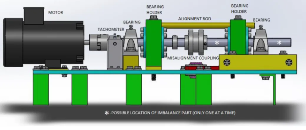
The test-bench (Figure 3) consists of an electric motor (MicroMax 56C FR) capable of producing consisting torque from 100-3600 RPM. The electric motor is coupled to a free-spinning shaft supported by two bearings, which is coupled with a second shaft through a rubber coupling mechanism and also supported by two bearings. The rubber coupling mechanism allows testing for shaft misalignment by shifting the base-plate supporting the second shaft (yellow block on far right of Figure 3).
A symmetrically shaped custom made part can be attached to the end of the shaft. A small weight can then be screwed to the side of this object to shift the center of gravity of the shaft. This introduces shaft imbalance.
A second internally damaged motor was also used for testing. The second motor's internal shaft was slightly misaligned, which caused damaging friction between internal components.
The main objective of the work presented in this paper is to design and test the novelty detector, and the information provided should serve as a proof of concept. Therefore, all experiments were designed accordingly.
All single audio samples were collected for 10 seconds at a sample rate of 44,100Hz from a 2.7Hz rotating shaft.
Figure 3: Test bench
3.2. Case Study: Illustrative Example
The following study provides an example of the basic operation of the novelty detector, and illustrates how nodes monitor the audio signals. This example only shows step 1 of training, and does not expand into establishing a novelty threshold. An audio sample from the rotating machinery was collected and used as the base original signal for training.
An impulse signal, modulated by 0.2Hz, with a carrier frequency of 4KHz, was digitally introduced to the original signal as a novelty. Lower energy 2nd (8KHz) and 3rd
(12KHz) harmonics were also introduced.
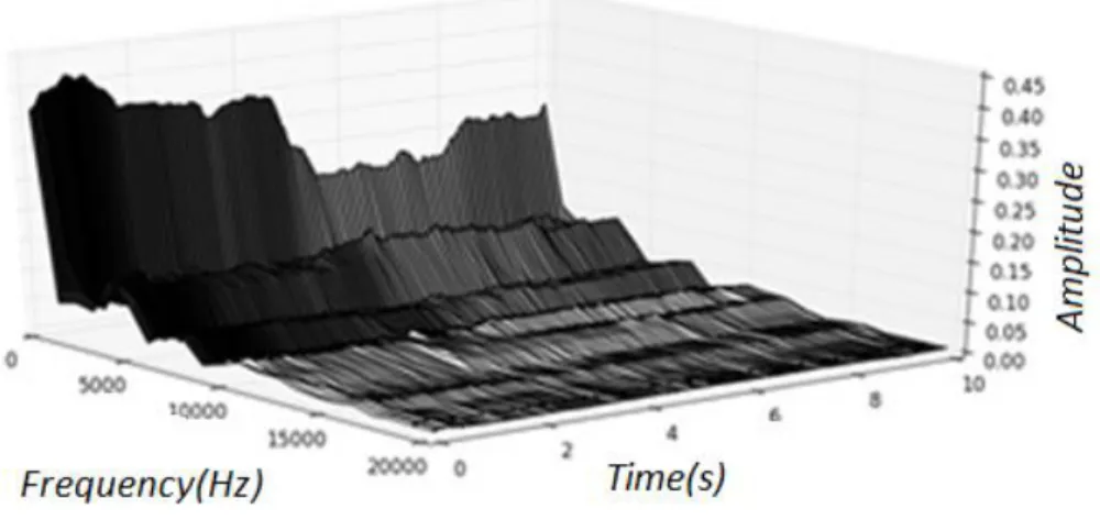
Figure 4 depicts a 10 seconds sample from the raw time domain signal before the synthetic novelty was introduced. Figure 5 shows a 10 second sample from the raw time domain signal after the subtle synthetic novelty was introduced.
It is clear that the rotating machinery's raw audio signal is noisy and of a chaotic nature. Figure 4 and Figure 5 look as if they were the exact same signal to the naked eye. The nature of the signals represented by Figure 4 and Figure 5 suggest that pre-processing
is strictly necessary to obtain a cleaner pattern and time-frequency information. The extreme similarities between both signals were chosen deliberately in order to easily explain the mechanisms of the algorithm, and to show its capabilities at detecting subtle novelties.
After the raw signals were processed with short-time FFT, the time-frequency pattern represented by Figure 6 was obtained. The novel energy pattern is difficult to detect by simply looking at Figure 6. This is because of the relatively low energy of the novelty compared to the rest of the pattern, but the overall time-frequency pattern
Figure 4: Original signal in time domain
contains more useful information than the time domain signals presented in Figure 4 and Figure 5. It is important to note that the time-frequency pattern provides both time and frequency information. For a sampling rate of 44,100Hz and a time window of 10 ms for the short-time FFT, there is a total of 220 frequency bins; bin = 40 includes energy from frequencies 4,000Hz-4,100Hz. It is known from the design of the experiment that novel time patterns should appear in bin = 40, bin = 80 and bin = 120 in Figure 6. Extracting and plotting the time-domain signal for bin = 40 from the time-frequency pattern, as shown by the time signals in Figure 7 and Figure 8 the differences in the patterns between healthy and novel signals are clearly visible.
Figure 7: Original signal at bin = 40 after short-time FFT
Figure 9: Original signal at bin = 80 after short-time FFT
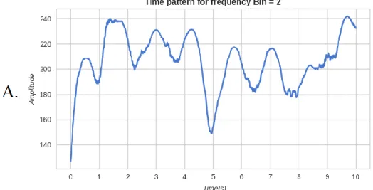
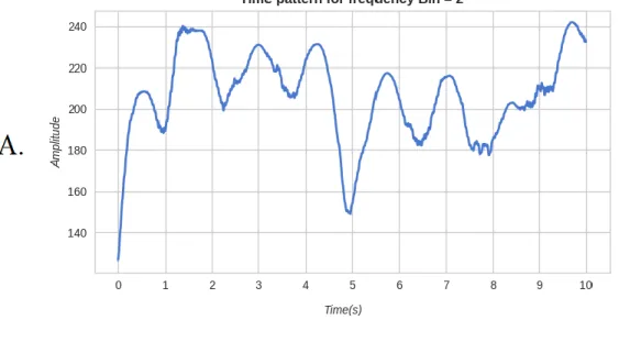
Figure 7.A depicts the time pattern at bin = 40 for the original signal, and Figure 7.B shows the probability density function of the energy estimated by the
monitoring node. Figure 8 illustrates the time pattern at bin = 40 for the novelty signal and its respective probability density function estimated by the monitoring node. Figure 8.A is equivalent to extracting and plotting bin = 40 from the time-frequency pattern shown in Figure 6. The lower images show the probability density functions estimated by kernel density estimation with a bandwidth of 0.75. Here, we can easily see the
differences between the time patterns and their respective probability density functions. Figure 9 and Figure 10 depict information obtained from the monitoring node at bin =
80, for normal and novelty signals, respectively. It is noticeable that due to the low energy of the 2nd harmonic, the differences are more subtle, yet still visually perceptible.
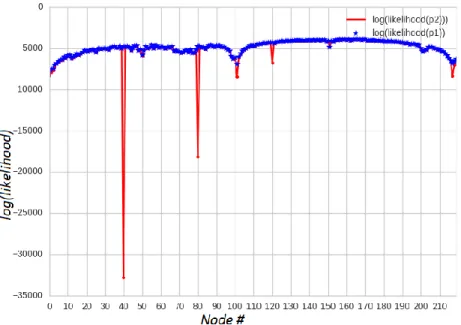
Figure 11 depicts the results obtained from each monitoring node. Here p1 (blue) stands for pattern 1 (original signal) and p2 (red) stands for pattern 2 (novelty signal). It is clear from these results that there is a novelty on bin = 40 and bin = 80. The monitoring node for the third harmonic (bin = 120) also shows differences, but not enough to argue a novelty exists on bin = 120. This is due to the very low energy of the novelty signal at 12Khz. It is important to note that Figure 11 presents results obtained from the novelty detector that has only received step 1 training. An optimal bandwidth and novelty threshold was not found for this case study.
3.3. Experimental Example 1: Conceptual Testing
In order to test the novelty detector as a proof of concept, an experimental investigation with the test bench was performed for the shaft rotating at 2.7Hz. Seven independent audio samples of 10 seconds each at 44,100Hz sampling rate were collected. The novelty detector was then trained. The first sample was used for step one training, and all other samples were used as the thresholding set for establishing the novelty threshold (training step three). Since this experiment was intended to quickly stablish the viability of this algorithm as a novelty detector, a single bandwidth of 0.75 was chosen for all nodes. An 8th novel audio sample with an introduced random novelty was
collected. Such novelty was introduced by randomly tapping a metallic element of the machine with a small wrench three times in the course of 10 seconds.
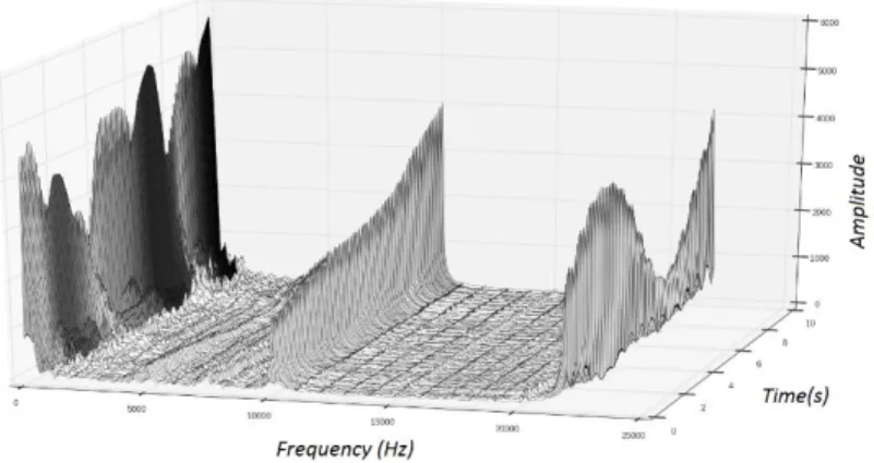
This was done to simulate a small metallic piece randomly impacting a component of the machine. Figure 12 and Figure 13 illustrate the results obtained from this experiment. The blue lines create an inside region of normal operating conditions,
and an outside region of novelty. This blue region is derived from the threshold training process. The red dots are the results obtained from the trained nodes when presented a new signal.
The red dots located outside the blue region indicate where in the frequency domain novelties occur. For this particular experiment, a total of 63 nodes out of 220 rejected the null hypothesis; detecting novel signals. The amount of nodes and their reported values indicate how different the new pattern is from the base signal. This information could potentially be used to predict the severity of a possible mechanical fault. A larger number of novel nodes and more negative reported likelihoods would indicate a more novel pattern, which could translate to a more severe, or obvious fault. Monitoring the novelty over time would be of crucial necessity. If a novelty keeps appearing over time, or results keep getting further from the base signal, it would be clear that the machine's sound signature has permanently changed. Otherwise, if the signal goes back to normal and the novelty does not occur again, it is very likely that the captured novelty is not related to a permanent change.
Figure 12: Trained novelty detector with normal signal results
Data were also collected for the machine rotating with the shaft misaligned, and with the damaged motor. 139 nodes raised novelties for the former, and 106 novelties were raised for the latter.
Another test consisted of taking an audio sample for the machine operating under normal conditions 2 weeks after the initial 7 healthy samples were collected. This new signal was then introduced as an input to the trained novelty detector. The trained algorithm raised only 9 novelty nodes, and the values reported by the nodes were relatively very close to the healthy region. The main objective of this experiment was to test the degradation of the algorithm over time. It is expected for the machine to slightly change its sound signature over time, which indicates that the network should be adaptive and retrained over time. Re-training a non-parametric based novelty detector can be easily performed [5]. These simple experiments show that the proposed algorithm clearly works for the purpose of novelty detection. The following experimental example shows a more in depth analysis of the novelty detector’s performance as well as the importance of the bandwidth parameter.
3.4. Experimental Example 2: Testing and Validating the Novelty Detector
For this experiment a total of 128 samples of 10 seconds were collected for the machine in normal conditions. To build the training data for training step 1, 10 random samples were drawn from the normal data pool. Then a random 1 second sample was sampled from each of the 10 samples. A 10 second training data sample was built by concatenating all the 1 second chunks, as explained by the first training step of the algorithm. This 10 second sample was then used for training step 1 and 2 of the algorithm.
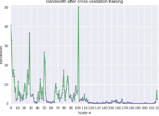
Then they were excluded from the initial pool of 128 testing samples. Another 30 random samples were taken from the pool of normal data, and used to compute the novelty threshold (training step 3). These samples were then excluded from the initial pool of normal data as well. The remaining normal data was left and used as the “normal” test validation set. Figure 14 shows the different bandwidths obtained for each node using the pseudo maximum likelihood estimation cross-validation technique.
Figure 14: Bandwidth parameter estimation
It is clear from Figure 14 that the optimal bandwidths across nodes can be very different. Figure 15 and Figure 16 show the difference in estimated probability functions using a general bandwidth of 0.75 and the optimal bandwidth found respectively for node 2. The figures show the respective time pattern for node 2 and the estimated P.D.F. with the histogram of the data on the background. It is clear that the bandwidth of 0.75 overfits
the data. It is important to note that using a general bandwidth for all nodes will not necessarily build a useless novelty detector, as it was shown in the previous example. As a proof of concept the novelty detector with a general bandwidth clearly works, but in practice there is a high risk some nodes would either underfit or overfit the training data. Overfitting occurs when the bandwidth is too small, which would lead to misclassified novelties; false alarms. Underfitting occurs when the bandwith is too large, which leads to high generalization; failure to detect novelties.
Four sets of “novel” test data were collected. For the first dataset the steel block barely establishes contact with the rotating shaft, which creates a barely audible signal. For this experiment, the steel block was pressed slightly into the rotating shaft, just so that the rotating shaft and the block would be in contact. This is a very generic type of fault and could be very difficult to detect with a deterministic model if caused by an unmonitored element. It also produces a non-stationary signal, which can be very difficult to detect from regular spectral analysis. For example, a bearing without proper lubrication would start to wear internally. This would increase metal to metal friction contact that would eventually lead to malfunction. Any component of the machine wearing due to unwanted contact would produce this type of signal. Therefore, this is a great experiment to evaluate the performance of the algorithm for generalized health monitoring, and machine degradation purposes. The audio signal is such that it could perhaps be learned and recognized by a trained ear.
For the second data set, the block was pressed against the rotating shaft with more force; creating a loud and audible signal. This simulates a more severe fault, and higher total novelty scores should be expected.
The third data set consisted on taking samples when the machine was operating in normal conditions, but an external loud novel source was present for a portion of the test data. In this case, a lathe which is 20 meters away from the machine being monitored was turned on and operated by a machinist.
Lastly, a fourth set of data was collected for the case of shaft imbalance. All data samples were collected in a machine shop during regular working hours to evaluate the
behavior of the algorithm when presented sources of novelties that do not represent a mechanical fault for the machine being monitored.
Table 1 shows the results obtained from the testing samples with the machine operating under normal conditions. The results are color coded so with a gradient going
from green to red. Where green is a TNS = 0, yellow a TNS = 5, and red a TNS = 10.
Figure 17: Total Novelty Score legend
On Table 1 each column represents the node range for the Total Novelty Score results, and each row represents a different sample. As can easily be seen on Table 1, most of the samples contain TNS below 10 for all frequencies. Only 5.7% of the table show TNS values over 10. This is expected, as external sources of audio would sometimes contaminate the data. However, it is clear that after a novelty occurs, the novelty scores go back to the green range, which should not occur in case of an actual permanent change of the machine’s audio signature.
Table 2 shows the results obtained from the first set of novel data. Novel audio signals were clearly detected. There is also a somewhat clear developing pattern on frequencies going from 3KHz to 4KHz, as well as some lower and higher frequencies. High frequencies are expected due to resonance of metallic elements.
The dynamics of the fault are very complex; there is of course the obvious impacts between the steel block and the rotating shaft. However, other components of the machine would resonate as well as vibrations are transferred from the shaft to other elements. The very high frequencies could be harmonics of the lower frequencies.
Table 3 shows the results obtained from the second set of novel data. Most of the table is clearly red, and the Total Novelty Scores are much larger than on the previous experiment. The algorithm has clearly succeeded in identifying a very clear signal that indicates a concerning degree of novelty. The sound signature of the machine has clearly permanently changed. It is important to note that 3 of the samples do not show a TNS larger than 10, which means that 15% of the table do not show a high degree of novelty. This is possibly due to the chaotic nature by which the fault releases energy. For this reason, it is very important to monitor the machine through time before elaborating conclusions about its condition. Following the principle that the machine’s sound signature must permanently change to stablish a fault might be present in the system.
Table 4 depicts how the novelty detector would behave if an external novel event occurred. For the first minute of data collection the lathe was on, and it is clear that the signal is deemed to be extremely novel by the novelty detector. The lathe is so loud and different that it completely changes the sound signature that is expected by the algorithm, the null hypothesis is rejected by most nodes of the novelty detector, and the Total Novelty Scores are quite high. However, after the first minute, once the lathe is turned off, it is clear how the novelty detector gradually goes back to normal. It goes back to normal as the machine completely shuts down and the machinist cleans the workspace and leaves the working area. Since novelty scores go back to normal. It is clear from the
results presented in Table 4 that the sound signature of the machine being monitored has not permanently changed.
Table 5 shows the performance of the algorithm by increasing the training sample size. In this case the training sample T for training step 1 was increased to 20 seconds by drawing 10 samples of T’ = 2 seconds from the normal operating conditions data pool. The algorithm did not perform better or worse, as 6.8% of the samples showed TNS larger than 10.
Table 6 shows the results obtained for the shaft imbalance experiment. It is clear from these results that the novelty detector succeeded in detecting the anomaly. The TNS shows a clear novel pattern for the lower frequencies. This is expected as shaft imbalance generally releases novel energy for lower frequencies. The pattern is also consistent; showing less randomness than seen by the previous faults. This is also expected as the imbalance fault is constant and presents periodic signals for every shaft revolution. As the machine starts to degrade and other components start to fail due to the shaft imbalance; it is expected that the novel signals will become more random and novelties will start to appear in other frequency bins.
Table 2: Friction between metal components – barely audible
CHAPTER 4: CONCLUSIONS
An audio novelty detector, designed for rotating machinery and inspired by the functionality of human audio pattern recognition, was conceptualized and tested. Experiments designed to build and test the algorithm proved the capabilities of the algorithm for novelty detection purposes. The structure of the probabilistic model presented in this thesis eliminates constraints originating from the curse of dimensionality [1].
The model could easily include a neural network classifier, as a probabilistic neural network could potentially be designed by establishing connections between the novelty detector's nodes. This could expand the capabilities of the system into classifying different fault modes and should be explored in future work. This model can also be tailored to expand its novelty detection capabilities for transient problems beyond the domain of machinery pattern recognition.
The nodes of the novelty detector monitor for anomalies by using the non-parametric Parzen Windows technique. This method is applied due to the computational speed advantage of statistical non-parametric techniques over neural network techniques, and their robustness in comparison with parametric methods [3] [2]. However, there exists a possibility that neural networks or other statistical techniques could perform better in situations where computational power is not necessarily a constraint [2].
For future work, different novelty detection techniques [3] [2] [18] can be used to train the nodes, and performance can then be compared with the probabilistic novelty detector presented in this research.
Other signal processing methods such as the discrete wavelet transform can be used to build the frequency bins, and should be explored in future work.
The method of “Pseudo log-likelihood cross-validation” was used to estimate the bandwidth parameter for each node of the novelty detector. This technique was applied for the final experimental testing. The method proved to successfully reduce the problem of overfitting the probability density function for each of the nodes. There are other bandwidth parameter estimation methods that should be studied and compared in future work related to this topic [13] [12].
Metrics to measure the degree of novelty of a new pattern such as the “Total
Novelty Score” and the “Individual Node Relative Difference” were defined and used to
present results for the final experimental testing. The metrics succeeded in condensing the output from the novelty detector and presenting a concrete measure of novelty. This can be used as information to infer a machine’s fault as a Shewhart’s “assignable cause” [14] to the novelties. Monitoring the machine over time also showed that false alarms do not change the learned sound signature permanently in accordance with the 2nd law of
thermodynamics, which can also be used as information to infer an assignable cause to the novelty.
Experiments showed the novelty detector to have great performance at learning the sound signature of a machine in a very noisy environment and successfully identifying novelties. The novelty detection technique presented in this thesis could greatly enhance the performance of current state-of-the art condition monitoring systems, or could also be used as a stand-alone system.
Bibliography
[1] M. J. Desforges, P. J. Jacob and J. E. Cooper, "Applications of probability density estimation to the detection of abnormal conditions in engineering," Journal of
Mechanical Engineering Science, vol. 212, pp. 687-703, 1998.
[2] M. Markou and S. Singh, "Novelty detection: a review-part 2: neural network based approaches," Signal Processing, vol. 93, no. 2, pp. 2499-2521, 2003.
[3] M. Markou and S. Singh, "Novelty detection: a review-part 1: statistical approaches," Signal Processing, vol. 83, pp. 2481-2497, 2003.
[4] R. O. Duda, P. E. Hart and D. G. Stork, Pattern Classification, United States of America: Wiley-Interscience, 2001.
[5] D. Y. Yeung and C. Chow, "Parzen-window network intrusion detectors," in
Proceedings of the international Conference on Pattern Recognition, Quebec,
Canada, 2002.
[6] E. Marchi, F. Vesperini, S. Squartini and B. Schuller, "Deep Recurrent Neural Network-Based Autoencoders for Acoustic Novelty Detection," Computational Intelligence and Neuroscience, 2017.
[7] C. K. On, P. M. Pandiyan, S. Yaacob and A. Saudi, "Mel-frequency cepstral coefficient analysis in speech recognition," in International Conference on Computing & Informatics, Kuala Lumpur, Malaysia, 2009.
[8] S. Mallat, A Wavelet Tour of Signal Processing, San Diego, CA: Academic Press, 1998.
[9] J. Hass, "An acoustics primer," Indiana University, 2003. [Online]. Available: http://www.indiana.edu/~emusic/acoustics/ear.htm. [Accessed 2017].
[10] B. Bagheri and H. L. R. Ahmadi, "Implementing discrete wavelet transform and ariticial neural networks for acoustic condition monitoring of gearbox," Elixir Mech. Eng, vol. 35, pp. 2909-2911, 2011.
[11] P. F, G. Varoquax, A. Gramfort, V. Michel, B. Thirion, O. Grisel, M. Blondel, P. Pretenhofer, R. Weiss, V. Dubourg, J. Vanderplas, A. Passos, D. Cournapeau, M. Brucher, M. Perrot and E. Duchesnay, "Scikit-learn: Machine Learning in Python,"
Journal of Machine Learning Research, vol. 12, pp. 2825-2830, 2011.
[12] R. Cao, Cuevas and G. W. A, "A comparative study of several smoothing methods in density estimation," Computational Statistics & Data Analysis, pp. 153-176, 1994.
[13] U. Byeong and J. S. Marron, "Comparison of Data-Driven Bandwidth Selectors," Journal of the American Statistical Association, vol. 85, pp. 66-72, 1990.
[14] W. A. Shewhart, Statistical Method from the Viewpoint of Quality Control, Toronto, Canada: General Publishing Company, Ltd, 1939.
[15] A. Zaknich, Neural Networks for intelligent Signal Processing, Singapore: World Scientific, 2003.
[16] P. Menon, A diagnostics approach for helicopter drive train systems, Burlington, VT: The University of Vermont, 2013.
[17] E. Bechhoefer and M. Kingsley, "A Review of Time Synchronous Average Algorithms," in Annual Conference of the Prognostics and Health Management, 2009.
[18] F. E. Grubbs, "Sample criteria for testing outlying observations," Annals of Mathematical Statistics, vol. 21, pp. 27-58, 1950.
[19] E. D. Angola, Audio novelty detection library, GitHub repository, https://github.com/eangola/AudioNoveltyDetector, 2018.