Electrical and Computer Engineering Publications
Electrical and Computer Engineering Department
9-25-2019
Similarity-Based Chained Transfer Learning for
Energy Forecasting with Big Data
Yifang Tian
Western University, [email protected]
Ljubisa Sehovac
Western University
Katarina Grolinger
Western University, [email protected]
Follow this and additional works at:
https://ir.lib.uwo.ca/electricalpub
Part of the
Artificial Intelligence and Robotics Commons
,
Computer Engineering Commons
,
Electrical and Computer Engineering Commons
,
Software Engineering Commons
, and the
Systems
Architecture Commons
Citation of this paper:
Tian, Yifang; Sehovac, Ljubisa; and Grolinger, Katarina, "Similarity-Based Chained Transfer Learning for Energy Forecasting with Big Data" (2019).Electrical and Computer Engineering Publications. 171.
Digital Object Identifier
Similarity-Based Chained Transfer
Learning for Energy Forecasting with
Big Data
YIFANG TIAN, LJUBISA SEHOVAC (Student Member, IEEE), AND KATARINA GROLINGER (Member, IEEE)
Department of Electrical and Computer Engineering, Western University, London, ON, N6A 5B9 CA (e-mail: {ytian285, lsehovac, kgroling}@uwo.ca)
Corresponding author: K. Grolinger (e-mail: [email protected]).
We acknowledge the support of the Natural Sciences and Engineering Research Council of Canada (NSERC), grant EGP 519910-2017
ABSTRACT Smart meter popularity has resulted in the ability to collect big energy data and has created opportunities for large-scale energy forecasting. Machine Learning (ML) techniques commonly used for forecasting, such as neural networks, involve computationally intensive training typically with data from a single building or a single aggregated load to predict future consumption for that same building or aggregated load. With hundreds of thousands of meters, it becomes impractical or even infeasible to individually train a model for each meter. Consequently, this paper proposes Similarity-Based Chained Transfer Learning (SBCTL), an approach for building neural network-based models for many meters by taking advantage of already trained models through transfer learning. The first model is trained in a traditional way whereas all other models transfer knowledge from the existing models in a chain-like manner according to similarities between energy consumption profiles. A Recurrent Neural Network (RNN) was used as the base forecasting model, two initialization techniques were considered, and different similarity measures were explored. The experiments show that SBCTL achieves accuracy comparable to traditional ML training while taking only a fraction of time.
INDEX TERMS Big Data, Deep Learning, Energy Forecasting, Gated Recurrent Units, Recurrent Neural Network, Smart Meters, Transfer Learning
I. INTRODUCTION
S
MART meters are being installed in industrial, com-mercial, and residential buildings at increasing rates: presently there are over 70 million smart meters in the USA and over 96 million in China [1]. A number of smart meters together with their possibly frequent reading intervals results in a massive quantity of electricity consumption data. These Big Data have created new opportunities for analyzing en-ergy use, designing demand-response programs, identifying savings opportunities, and measuring energy efficiency, but they also caused challenges related to processing such large data.Energy forecasting has been attracting significant research interest because of the increased importance of preserving the environment, availability of smart meter data, and forecasting importance for both, retailers [2] and consumers [3]. Sensor-based energy forecasting relies on historical data from smart meters or other sensors, often in conjunction with meteo-rological information, to infer future energy consumption.
Examples of Machine Learning (ML) techniques used for this task include Neural Networks (NN) [4], Support Vec-tor Machine (SVM) [4], and their variants [5]. These ML techniques achieve good accuracy [1]; however, they are typically computationally complex and, with a high number of readings, it may be time-consuming to train a prediction model even for a single building/meter [6].
Recently, Recurrent Neural Networks (RNN) have out-performed other energy forecasting models [7]. An RNN is a type of NN where connections span adjacent time steps and form a directed graph along a temporal sequence. This makes them suitable for capturing time-dependencies and for dealing with time series data such as smart meter data. Because of spanning adjacent time steps, the total number of connections among neurons in an RNN is larger than in a traditional feed-forward neural network. Consequently, the number of weights to learning during training is increased, and so is the training time.
Many machine learning techniques, including RNNs,
quire training a forecasting model with historical data from a single building or a group of buildings to predict future consumption for that same building or the group of buildings. As training even a single forecasting model can be compu-tationally expensive and time-consuming [6], repeating the same process for hundreds of thousands of meters becomes impractical or even infeasible.
Transfer learning has been identified as one of the open re-search areas in smart meter data analytics [1]; it is motivated by the fact that people can intelligently apply knowledge learned in the past to solve new problems in a new context in a faster and/or better way [8]. In traditional ML, models are built for a specific domain (e.g. specific smart meter) and task (e.g. energy prediction), and then used for the same domain and task (e.g. predict future consumption for the same meter). On the other hand, transfer learning aims to take advantage of knowledge gained on one domain/task and apply it to a different domain/task. Consequently, transfer learning has the potential to enable training machine learning models for many meters/buildings without the computational cost involved with training each model separately.
This paper proposes Similarity-based Chained Transfer Learning (SBCTL), a novel solution for building neural network-based forecasting models for a large number of smart meters. The model for the first meter is trained in a traditional manner using a Sequence-to-Sequence RNN; hyperparameters are optimized and weights learned using data from that meter. Next, the model is built for the meter with the energy consumption pattern the most similar to the pattern of the first meter, but the training process starts with the pre-trained model from the first meter. The process continues in a chain-like manner according to similarities in energy consumption patterns. Note that the SBCTL objective is not to improve accuracy for an individual meter, but to reduce training time when dealing with many meters. In the three experiments with different data sets (one with over 400 smart meters), SBCTL achieved accuracy comparable to traditional NN models while taking only a fraction of time.
The rest of the paper is organized as follows: Section II describes the background, Section III discusses the related work, Section IV presents SBCTL, Section V explains the experiments and corresponding results, and finally Section VI concludes the paper.
II. BACKGROUND
This section introduces the feed-forward and recurrent neural networks and presents transfer learning concepts.
A. FEED-FORWARD AND RECURRENT NEURAL NETWORKS
Feed-forward neural network (FFNN) consists of intercon-nected neurons organized in an input layer, hidden layer(s), and an output layer [9]. Neurons in each hidden layer are fully connected with neurons in the preceding and the sub-sequent layer; however, there are no connections among neurons in the same layer. The training process starts with
initializing weights w between neurons to random values [9]; this initial state if referred to as the seed. The training samples are passed forward through the network and back-propagation is applied to minimize the objective function by updating the weights w [9]. An epoch refers to one forward pass and one backward pass of all training data; training typically requires a number of epochs for weights to converge. When the weights are updated using gradient descent, there is a possibility of getting stuck in a local minimum. To avoid this, training is often repeated by starting from different initial random states or seeds.
Recurrent neural networks (RNNs) are NN where connec-tions between nodes form a directed graph along a temporal sequence [9]. RNN cells contain internal states capable of remembering information in sequential time steps, which makes them well-suited for time series forecasting tasks such as energy prediction. In traditional RNNs, the weights w
are updated using back-propagation through time (BPTT) algorithm; however, this method suffers from the vanishing gradient problem [10]. To overcome this problem, the Long-Short Term Memory (LSTM) cell was designed [9]. To simplify LSTM while still maintaining the core functionality, the Gated Recurrent Unit (GRU) cell was introduced [11]. GRU cells compute reset gater, update gatez, cell activation
k, and hidden statehas [11]:
r[t]=σ(Wxrx[t]+bxr+Whrh[t−1]+bhr) (1)
z[t]=σ(Wxzx[t]+bxz+Whzh[t−1]+bhz) (2)
k[t]= tanh(Wxkx[t]+bxk+rt(Whkh[t−1]+bhk))
(3)
h[t]= (1−z[t])k[t]+z[t]h[t−1] (4)
whereσis the sigmoid activation function,tanhis the hy-perbolictanhactivation function, andrepresents element-wise multiplication. The input-hidden weight matrices are
Wx’s and hidden-hidden weight matrices are Wh’s.
Simi-larly, thebx’s andbh’s are the corresponding biases.
Sequence-to-Sequence (Seq2eqS) RNNs have been ex-tensively used for language translation and recently have demonstrated success in energy forecasting [7]. They consist of two RNNs, an encoder and decoder RNN. This struc-ture improves consecutive sequence prediction and allows Seq2Seq RNNs to have varying input and output lengths. Seq2Seq RNN can be used with LSTM or GRU cells.
B. TRANSFER LEARNING
Transfer learning is a machine learning approach where knowledge gained while performing a task in one domain is used to improve learning in a different domain or applied for a different task [8]. It is defined as follows [8]:
Definition1 (Transfer Learning):Given a source domainDS
and learning taskTS, a target domainDT and learning task TT, transfer learning aims to help improve the learning of the
target predictive function rT(·)inDT using the knowledge
Here, a domain is a pair D = {F, P(X)}, where F = {f1, ..., fk}is a feature space,Xis a set of learning samples X = {x1, ..., xm}, and P(X) is the marginal probability
distribution ofX. Domains are considered different if either marginal probability distributions or feature spaces are dif-ferent.
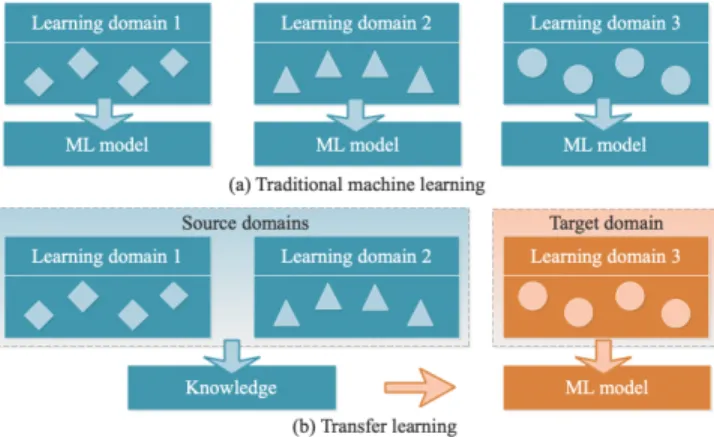
Fig. 1 illustrates the difference between traditional ma-chine learning and transfer learning. The traditional ML algo-rithms learn from a single domain for each model separately, whereas transfer learning uses the knowledge gained from multiple source domains to improve learning on the target domain. Different knowledge, such as instances, parameters, and relational knowledge, can be transferred across tasks and domains [8] .
In the energy forecasting with smart meter data, there is a single task (energy forecasting), but there are differ-ent domains: smart meters are considered differdiffer-ent domains because they differ in energy consumption patterns and marginal probability distributions. SBCTL proposed here transfers weights and hyperparameters learned on the source domain (meter) to improve learning on the target domain. Thus, SBCTL belongs to the category of parameter transfer approaches.
III. RELATED WORK
Many approaches have been used for sensor-based energy forecasting; examples include fuzzy Bayesian [12], Support Vector Machine (SVM) [13], neural network [4] and ARIMA [14]. Tang et al. [12] were interested in predicting energy on an annual basis and they proposed probabilistic energy forecasting based on fuzzy Bayesian theory and expert pre-diction. Grolinger et al. [6] combined local learning with support vector regression (SVR) to reduce computation time while maintaining forecasting accuracy. Amber et al. [4] compared Multiple Regression (MR), Genetic Programming (GP), Artificial Neural Network (ANN), Deep Neural Net-work (DNN), and Support Vector Machine (SVM). Artificial Neural Network achieved better accuracy than the remaining four algorithms.
FIGURE 1: Traditional machine learning and transfer learn-ing.
Several algorithms were combined to form ensemble learning models. Li et al. [15] proposed teaching-learning based optimization with artificial neural network for hourly energy prediction. Khairalla et al. [16] investigated Stack-ing Multi-LearnStack-ing Ensemble (SMLE) model and combined Support Vector Regression (SVR), neural network, and linear regression learners. Baesmatet al.[5] proposed the weighted combination of ARIMA and RELM for city-level energy forecasting.
In recent years, recurrent neural networks have gained popularity in forecasting because of their ability to cap-ture time-dependencies. Han et al.[17] proposed wind and photovoltaic power generation prediction based on copula function and LSTM network whereas Jiao et al. [18] de-signed multiple sequence LSTM RNN for non-residential load forecasting. Bouktif et al. [10] also used LSTM for energy forecasting but they combined it with genetic al-gorithm (GA) to find optimal time lags and the number of layers for the LSTM model. Standard LSTM was com-pared to Sequence-to-Sequence (Seq2Seq) architecture [19] and on one-minute time-step resolution datasets, Seq2Seq performed better. Similarly, in experiments performed by Sehovacet al.[7], Seq2Seq RNN also outperformed standard RNN.
As can be seen, the use of NN-based solutions has been quite popular [7], [10], [15]–[19] and recently Seq2Seq RNN provided increased prediction accuracy [7], [19]. Neverthe-less, all the reviewed NN approaches focus on building a prediction model for a specific building or an aggregated load using historical data from that same building or the same aggregated load. In contrast, our work aims to reduce computation needed to create prediction models for a large number of smart meters taking advantage of transfer learning. Transfer learning has been applied in different domains and for different tasks. For visual recognition, Zhu et al. [20] proposed a weakly-supervised cross-domain dictionary learning method. In Natural Language Processing (NLP), Hu et al. [21] improved mispronunciation detection with a deep neural network trained acoustic model and transfer learning-based Logistic Regression classifiers. In software engineering, Ma et al. [22] and Namet al. [23] addressed cross-company software defect classification. In contrast to domain-specific solutions [20]–[23], Liet al.[24] aimed to develop a transfer learning model for a variety of applications and presented augmented feature representations for domain adaptation. Similarly, Mozafariet al.[25] were interested in transfer between different domains and proposed a SVM-based model-transferring method for heterogeneous domain adaptation. These works [20]–[25] focus on feature augmen-tation whereas our work belongs to the parameter transfer category as it transfers model parameters.
Parameter transfer is often found associated with pre-trained neural networks in computer vision [8]. Krizhevsky et al. [26] trained ImageNet, a large, deep Convolutional Neural Network (CNN) for classifying 1.2 million pictures. It is computationally expensive and time-consuming to train
such a neural network with 650,000 neurons and 60 million parameters; nevertheless, once such a network is trained, it is a good foundation for other image classification problems. Menegolaet al. [27] used pre-trained ImageNet to develop an approach for melanoma screening. Similarly, a pre-trained AlexNet, another deep CNN architecture, was used to detect pathological brain in magnetic resonance images [28]. These parameter-transfer approaches deal with image classification whereas SBCTL addresses forecasting with time series data. In the energy domain, Mocanuet al.[29], Grubingeret al. [30], and Ribeiroet al.[31] applied transfer learning to pro-vide prediction models for buildings with limited historical data by using data from other similar buildings with rich data sets. Wile those studies [29]–[31] aim to solve the limited data issue for target buildings, our objective is to reduce computation needed to train prediction models for a large number of buildings.
IV. SIMILARITY-BASED CHAINED TRANSFER LEARNING
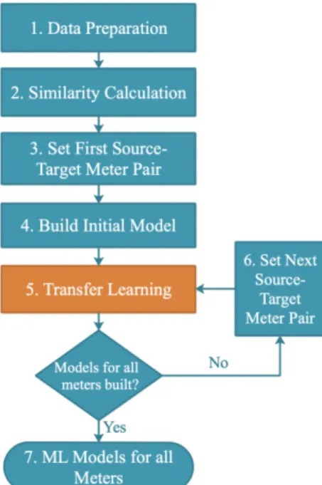
This paper proposes the Similarity-Based Chained Transfer Learning (SBCTL) approach for building neural network-based energy forecasting models for a large number of buildings by applying transfer learning. The approach takes advantage of the initial neural network model trained with a single meter data to initialize training models for other smart meters. SBCTL is illustrated in Fig. 2 and details of each stage are described in the following subsections.
A. DATA PREPARATION
The smart meter data typically contain energy readings such as consumption and demand, and the corresponding date and
FIGURE 2: Similarity-Based Chained Transfer Learning (SBCTL).
time. If the reading intervals are different, all smart meter data are processed to make intervals between the readings the same. In the case of energy consumption, meters with finer reading granularity are converted to a coarser granularity by adding consumption readings.
Whereas feature selection is often considered in energy forecasting studies [32], SBCTL does not include it, as SBCTL is primarily designed for forecasting using smart meter data with limited number of features; in experiments we used only seven features. Nevertheless, when working with more features, SBCTL could be augmented by adding feature selection step.
Let us denote this meter data as m1, m2, ..., mk ∈ M,
where M is the set of all meters and k is the number of meters. This data is processed into two data sets: the similarity set D and the forecasting setG. Meterndata in
Dis denoted asdn,dn ∈D, and the same meter data inGis
denoted bygn,gn ∈G. Although bothdnandgn belong to
the same meter, they are different in the number of features and time spans.
Similarity set D is created for calculation of similarities among energy consumption patterns recorded by different meters. It contains only energy consumption readings with-out any additional features because similarity is concerned solely with usage patterns. To capture quarterly and monthly patterns, D set must contain at least one year of energy readings. Each meter datadnmust start at the same date/time
to ensure alignment of temporal patterns.
Forecasting setG, in addition to energy readings, contains other features generated from date and time such as day of the year, and weekday/weekend. Data pre-processing for this set depends on the type of the forecasting model used. As Sequence-to-Sequence (Seq2Seq) RNNs [7] have shown great results in energy forecasting for individual smart me-ters, they are used in SBCTL to build the initial model as well as to refine transferred models.
To enable the use of Seq2Seq RNN, data is prepared applying the sliding window techniques proposed by Sehovac et al.[7]. One input sample consists of a matrixX ∈RT×f,
whereTis the length of the input sequence or the number of time steps in a window andf is the number of features. Note that energy readings for all time steps of the input sequence are included as input features. If the input sample ends at time t, the corresponding target sequence consists of load values for time stepst+ 1tot+N. This way,T time steps are used to predict the next N time steps ahead. The next sample is generated by sliding the window for one time step and repeating the same process.
The forecasting set is divided into training and test sets: first 80% of data is assigned for training and the last 20% for testing. This way, older data is used to train the model, and newer (test) data is used to evaluate and compare models. To capture monthly and quarterly patterns, the training set must contain at least one year of data; thus, the forecasting setG
contains at least 15 months of data.
Algorithm 1SBCTL
1: Input:SetM consisting of all meter data, initialization
2: Output:Models for all meters
3: D←transform1 (M) // similarity set
4: G←transform2 (M) // forecasting set (training)
5: D←normalization(D)
6: L(di, dj)←similarity(di, dj), for alldi, dj∈D, i < j
7: T ←M // initialize target set
8: S← {}// initialize source set
9: if initialization == A // From the most similar pair
10: (p, q)←arg min i,j
L(di, dj), f or di, dj ∈D, i < j
11: elseifinitialization == B // From the center
12: dcenter←mean(di), fordi∈D
13: p←arg min i L(di, dcenter), fordi∈D 14: q←arg min i L(dp, di), fordi∈D, i6=p 15: mm
p ←train initial model formpwithgpdata
16: S=SS
{mp} // add to source
17: T =T /S // remove from target
18: while T 6={}do
19: mmq ←transfer learning (mmp) withgq data
20: S =SS{mq} // add to source
21: T =T /S // remove from target
22: if T 6={}
23: (p, q)←arg min
i,j
L(di, dj), f or mi∈S, mj ∈T
24: Return:Models for all meters {mm
1, mm2...mmk}
1. For simplification, in the algorithm, G refers to only the training part of the forecasting set. The approach starts with data preparation, specifically by creating setsDandG, lines 3 and 4, and continues with the steps described in the remaining subsections.
B. SIMILARITY CALCULATION
Similarity calculation gives a numeric value to similarities between each possible pair of meters. Here, we are interested in energy patterns and not in the actual values of energy consumption. Therefore, all values from similarity data set
Dare first scaled to bring them to the same range (line 5 in Algorithm 1). Min-max normalization is performed for each meter separately resulting in each meter values in [0,1] range. Next, similarity between all pairs of meters is calculated (line 6, Algorithm 1); four different metrics are considered. Euclidean, Cosign, and Manhattan distances between meteri
andjare calculated as follows:
LEucl(di, dj) = v u u t N X t=1 (dt i−dtj)2 (5a) LCosign(di, dj) = 1− PN t=1(d t idtj) q PN t=1(d t i)2 q PN t=1(d t j)2 (5b) LM anh(di, dj) = N X t=1 |(dti−dtj)| (5c) f or di, dj∈D, i < j (5d)
The fourth metrics considered is Dynamic Time Warp-ing (DTW) distance [33]. DTW was selected because it is capable of measuring similarity between the two temporal sequences which may vary in speed. A well known example of a DTW application is automatic speech recognition where DTW is capable of handling different speaking speeds. In energy data, DTW could potentially capture peak shifts or prolonged peak periods. To control how much the sequences can be "warped" for the comparison calculation, a locality constraint referred to as the window is commonly added. In our work, experiments consider different window sizes in order to examine their impact on the forecasting accuracy.
For k number of meters, the outcome of the similarity calculation is a k∗k upper oblique matrix; this similarity matrix is denoted as Sk∗k
im . The lower the distance value
between two meters, the more similar are the meters. C. SET FIRST SOURCE-TARGET METER PAIR
The main idea behind SBCTL is to use a similarity measure to determine the source and target meters for the transfer process. To start with, none of the meters have an associated prediction model. Therefore, as indicated in lines 7 and 8, Algorithm 1, all meters belong to the target set T and the source set S is empty. Throughout the process, the target set will always have only the meters that do not yet have the corresponding prediction model and the source set will contain meters with an already trained model. Two different initialization techniques are considered:
InitializationA:Starting from the pair of the most similar meters. As indicated in Algorithm 1, line 10, the two meters that correspond to the minimum value in the similarity matrix
Skim∗k are assigned as a starting source-target pair (p, q). Either one of the two meters in the pair can be set as the sourcep; experiments will evaluate switchingpandqin the first source-target pair.
InitializationB:Starting from the meter that is the closest to the center. First, the center is calculated from the similarity data setD(Algorithm 1, line 12). For each time steptin the similarity set, the arithmetic meandt
centeris calculated as:
dtcenter = 1 k k X i=1 dti (6) VOLUME x, 2019 5
wherekstands for the number of meters anddt
iis a reading
from meteriat time stept.
The meter that is the closest to this center C according to selected similarity metrics is chosen as the initial meterp
(Algorithm 1, line 13). The meter that is the most similar to the initial meter pis selected as meterq(Algorithm 1, line 14).
D. BUILD INITIAL MODEL
This step is responsible for building the first prediction model which will serve as a starting point for the transfer learning. The initial model is built for the meter that was assigned as the sourcep(line 10 or 13, Algorithm 1). As indicated in line 15, the initial model for metermpis trained using forecasting
data setgp.
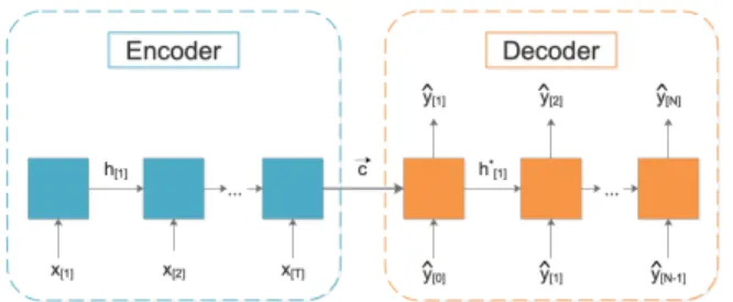
SBCTL is designed for NN-based algorithms; therefore, all models, including the initial one, must be built using a same NN approach. Specifically, a Seq2Seq RNN [7] is used because of its recent success. A Seq2Seq RNN [7] consists of an encoder RNN and decoder RNN as illustrated in Fig. 3. An input sequencex[1], ..., x[T]is passed through the encoder
RNN to obtain an encoded representation of the input vector referred to as the context vector (~c). The decoder RNN extracts information from this context vector at each output time step to obtain the prediction sequence {yˆ[1], ...,yˆ[N]}.
The initial input for the decoder RNN is the context value
ˆ
y[0]derived from the context vector.
This first model is trained in a traditional way: weights are initialized to random values and model is trained for a sufficient number of epochs ensuring that weights converge. To avoid local minimum, the process is repeated starting with a different set of random initial values referred to asseeds. The best model among all runs with different seeds is chosen for forecasting and used in the following SBCTL steps.
NN hyperparameters such as a number of layers and neu-rons, are also tuned in this step by splitting the training data into the training and validation sets; model selection is done on the validation set. After tuning hyperparameters for the initial model, they remain the same throughout the transfer learning and for all meter models. In contrast, the weights learned during the initial model training are used as a starting point for other models, but the weights do change.
The result of the training and tuning is the prediction
FIGURE 3: Sequence-to-Sequence Recurrent Neural Net-work.
model for meter pdenoted asmm
p (Algorithm 1, line 15).
Note thatmp indicates meter data for the meterpandmmp
denotes the trained model for the same meter p. Because meter pnow has the forecasting model, it is added to the set of source metersS, line 16, and removed from the set of target metersT, line 17. This initial model is now available for transfer learning.
E. TRANSFER LEARNING The initial modelmm
p is used as a seed for building all other
prediction models through transfer learning. The assumption is that if the meters share some similarity, so should their trained models. Thus, if we use the initial prediction model as a starting point for building the model for the most similar meter, the training should be reduced.
The meter to transfer knowledge to is the q meter from the (p, q) pair. Because the pair is determined according to similarities, SBCTL ensures that the transfer happens between more similar meters. As indicated in line 19, existing model mm
p trained previously for meter p and with data
set gp, is now used as a starting point for building meter q model. Model mm
p continues training, but now with the
target meter datagqto obtain modelmmq . Network structure
and hyperparameters determined during training for the first meter remain the same throughout the transfer learning and for all forecasting models. The weights from the source meter model mmp are transferred to the target meter q, but they change through training with the target meter data gq.
The number of training epoch needed for the weights to converge is lower because the training starts from the pre-trained weights.
If the two meters from the pair are very similar, the trans-ferred model, without any training with the target meter data, may already provide reasonable accuracy: we refer to transfer without additional training as epoch 0. The evaluation will explore how many epochs with target data are needed to achieve comparable accuracy to traditional NN training.
The result of the training with the transferred model is the new modelmmq , line 19. Next, as meter qnow has the
forecasting model, it is added to the set of source metersS, line 20, and removed from the set of target metersT, line 21. This additional model now is available for transfer learning.
If there are still meters that do not have a corresponding prediction model, in other words, if the target set T is not empty (lines 22 and 18), the SBCTL will proceed to Set Next Source-Target Meter Pair step. If forecasting models are trained for all meters, the SBCTL process is completed.
F. SET NEXT SOURCE-TARGET METER PAIR
In this step, the next source-target meter pair (p, q) is se-lected for transfer learning. As indicated in the algorithm’s name SBCTL, the processed is chained: building the next forecasting model depends on the previously built models. In each loop of the chained process, the forecasting model will always be transferred from one meter in the source setS
To determine which model should be trained next, the similarity distances calculated in line 6 are used. Because the transfer needs to happen from an already trained model, we are interested in finding a meter from the target setT that is the most similar to any meter in the source setS. Thus, line 23 in Algorithm 1 finds the pair with minimum distance L
under the constraint thatmp ∈ S andmq ∈ T. The model
will be transferred from frommptomq.
When the next source-target pair (p, q) is set (line 23), SBCTL continues to transfer learning, line 19, described in subsection IV-E.
G. ML MODELS FOR ALL METERS
This is the final output of the SBCTL process. As indicated in line 18, the transfer learning process completes when the target set is empty T = {} and all meters belong to the source setS. The algorithm results are the trained ML models for all metersmm
1, mm2...mmk.
V. EVALUATION
This section introduces the evaluation process, describes the three experiments with different data sets, and discusses the findings. Experiments one and two consider smaller data sets consisting of 7 and 19 meters, respectively. A small num-ber of meters in these two experiments allows for detailed examination of the transfer process as well as for accuracy comparison for each individual meter. On the other hand, the third data set consisting of 456 meters allows for evaluation at scale and demonstrates SBCTL forecasting accuracy and time savings with larger data. The used hardware was differ-ent for each data set and reflects the increase of data set size. All of the experiments applied SBCTL with initializations A and B. Also, Euclidean, Cosine, Manhattan, and DTW distance with window size of 3, 6, 12, and 24 were eval-uated. SBCTL was implemented using Python with Pandas and PyTorch libraries. GRU cells were used in Seq2Seq RNN because they achieved higher accuracy than LSTM in single meter forecasting [7]. The hyper-parameters used for the initial model as well as for all other models were: Hidden dimension size = 64, Batch size = 256, Epochs = 10, Optimizer = Adam, Learning rate = 0.001, Encoder size = 8 and Decoder size = 4.
A. EVALUATION PROCESS
For each meter in each experiment, SBCTL was compared to the traditional machine learning:
• Traditional ML. For each meter, an individual Seq2Seq
RNN model was trained using that meter training data. The process was repeated with 10 seeds and the model with the best MAPE was selected for comparisons. As a large number of models from the two experiments converged around the 10th epoch, the comparison was carried out with 10 epochs. For each epoch, the model was tested on the test set and accuracy was recorded.
• SBCTL. The models are built using SBCTL approach. In each experiment, the first model is built using the
traditional approach. All other models are built using SBCTL transfer learning and only trained for 5 epochs because the training starts from the pre-trained weights. For each epoch, including 0 epoch (no training on tar-get), the models were tested on the test set and accuracy was recorded.
To evaluate model accuracy, Mean Absolute Error (MAE) and Mean Absolute Percentage Error (MAPE) were selected because of their frequent use in energy forecasting studies [1]: MAE= 1 N0 N0 X t=1 |yt−yˆt| (7) MAPE=100% N0 N0 X t=1 yt−yˆt yt (8) whereyis the actual value,yˆis the predicted value, andN0
stands for the number of test set samples.
Other metrics such as Mean Absolute Error (MSE) and Root Mean Square Error (RMSE) were also calculated in the experiments, but they are not shown here as they exhibit the same patterns as MAE and MAPE.
B. EXPERIMENT ONE
This experiment was performed on MacBookPro with 2.9 GHz Intel Core i7 processor and 16 GB LPDDR3 memory.
1) Data set
Experiment one used a private data set from seven real-world meters measuring commercial buildings energy consumption in 15 min intervals. This data set, as well as data sets in remaining experiments, consist of reading date/time with corresponding energy consumption. For experiment one, the total number of readings was: 4 readings in one hour ×24 hours×487 days=46,752 for each meter.
Daily consumption profiles for meters 4 and 5 are depicted in figures 4 and 5, respectively. Meter 4 shows different pat-terns for weekend and weekdays, whereas meter 5 displays similar patterns for all days (no weekday/weekend distinc-tion) but different from meter 4. Although the patterns and average consumption are different among meters, SBCTL is able to transfer knowledge among the models.
2) Experiment
The similarity setD contained one year of energy readings without any additional features. The forecasting set G con-tained additional generated features (month and day of the year, day of the month, day of the week, weekend, hour, season, holiday) and included readings from all 487 days. A few samples fromGare shown in Table 1.
In Similarity Calculation step, the usage readings were normalized and the distance matrices were calculated. Set First Target-Source Meter Pair step with initialization A selected meters 2 and 4 as the meters with the smallest dis-tance; thus, the first pair can be(2,4)or(4,2). Experiments
TABLE 1: Example Data from Forecasting Data Set
Index Month Day of Year Day of Month Weekday Weekend Holiday Hour Season Usage (kW)
0 6 158 6 0 0 0 0 3 881.36
11661 10 279 5 2 0 0 11 4 1507.47
42978 8 239 27 6 1 0 16 3 983.60
FIGURE 4: Daily load profile - meter 4.
FIGURE 5: Daily load profile - meter 5.
were performed for both transfer paths (2,4) and (4,2). With initializationB, the initial meter was meter4, and the transfer path was the same as for initializationA with4as the starting meter. Here, the following steps are described assuming (4,2) order. The experiments were performed for both transfer paths(2,4)and(4,2).
Next, in Build Initial Model step, the model for meter 4 is trained with the training part ofg4. After the best modelmm4
for meter m4was completed,m4was removed from target
setTand added to source setS.
In Transfer Learning step, modelmm
4 was transferred to
meter 2 makingmm
2. The modelmm2 was first tested directly
on the test set ofg2(transfer 0 epoch) and then trained with
the training set ofg2for 5 epochs. Upon completed training,
m2 was removed from the target setT and added to source
setS.
Next, Set Next Source-Target Meter Pair step determines the order of remaining transfers. In this experiment, initial-izationAwith the first meter4and initializationBshared the same chained transfer path presented in Table 2. The first row indicates transfer from meter 4 to meter 2; the second row shows transfer from meter 2 to 7, and so on. The pairs were chosen to satisfy the condition of minimum distance value under constraints that one meter belongs to the source setS
and one to the target setT as indicated in line 18, algorithm
1. The process ends when all meters have the corresponding prediction model.
3) Result
The main objective of the experiments is to compare SBCTL accuracy with that of traditional machine learning when the model is trained for each meter individually. Thus, SBCTL is deemed successful if it is able to achieve similar accuracy to traditional ML but with reduced computation.
Fig. 6 compares the accuracy of SBCTL and traditional ML in terms of MAE for the six meters. Meter 4 is not included because it was the initial meter and, thus, follows the traditional ML training. The horizontal dashed line indicating the SBCTL accuracy at 5 epochs is included to ease visual comparison. It can be seen that when the model is transferred without additional training (epoch 0), MAE is relatively high. Nevertheless, MAE drops sharply in epochs 1 and 2, and after 5 epochs, 5 out of 6 meters achieve better accuracy than the traditional ML and the sixth meterm6achieves MAE within
0.01 difference. Moreover, after 3 epochs, all meters achieve accuracy comparable to traditional ML.
In addition to accuracy, it is important to compare compu-tational cost; thus, the average elapsed time, standard devia-tion, and variance for traditional ML and SBCTL are shown in Table 3. For SBCTL, the initial meter 4 is not included as it is trained in a traditional way. It can be observed that for SBCTL with three epochs, time was reduced to 10.48s from 365.47s achieved with traditional ML what is about 97% reduction. Note that traditional training was repeated with 10 different seeds (initializations) while the SBTCL starts from the single initial state transferred from an already trained meter.
For the initial pair or meters (4,2), two paths are possible;
TABLE 2: Experiment One: Chained Transfer Path
Step Source Meter Target Meter Euclidean Distance
1 m4 m2 135.2 2 m2 m7 135.5 3 m4 m6 160.4 4 m4 m1 202.9 5 m1 m5 198.4 6 m5 m3 264.0
TABLE 3: Experiment 1: Average Training Time Traditional SBCTL epoch
10 0 1 2 3 4 5
Time (s) 365.47 0 3.53 7.00 10.48 14.09 17.64 Std.Dev 0.13 0 0.07 0.08 0.11 0.21 0.32 Variance 0.018 0 0.005 0.006 0.012 0.046 0.100
FIGURE 6: Experiment 1: Test set MAE for SBCTL and traditional ML.
FIGURE 7: Experiment 1: Test set MAPE for the two SBCTL paths.
starting with meter 4 or with 2 as the initial meter. Irrelevant of the starting meter, the transfer path, Table 2, remained the same with the exception of the source and target reversal in the first row. Fig. 7 shows the comparison between the two SBCTL paths with 3 epochs and traditional ML: MAPE was used in contrast to MAE used in Fig. 6 to bring all errors to similar scales. Meters 2 and 4 are missing the bar for the path in which they were used as the initial meter and therefore trained in a traditional way. Both paths resulted in similar MAPE values; moreover, MAPE values were comparable to those achieved with traditional ML.
Overall, in experiment one, SBCTL achieved similar accu-racy to traditional ML while taking only about a fraction of time.
C. EXPERIMENT TWO
This data set is larger; thus, the experiment was performed on a computer with 3.80 GHz Intel i7-9800X processor, 32 GB RAM, and NVIDIA GeForce RTX 2080 Ti graphics card. GPU acceleration was used for training ML models.
1) Data set
This experiment used an open source data set [34] containing readings from 20 meters recorded in the one-hour intervals. Readings from the same 487 consecutive days were taken for each meter:24×487=11,688 readings for each meter.
2) Experiment
The same process was used as in experiment one. Meter7had the same readings as meter3for all time steps; thus, meter3
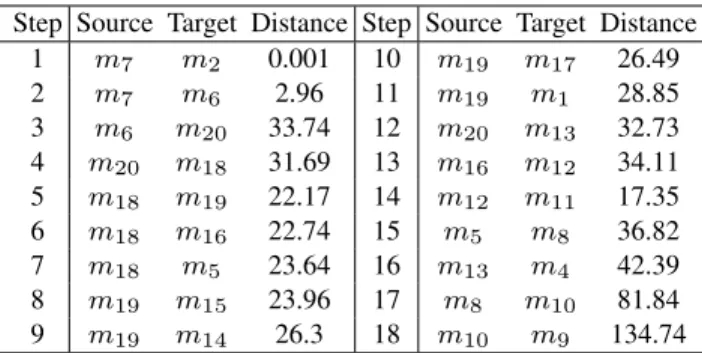
was removed from further evaluations. The chained transfer path for Euclidean distance is shown in Table 4.
3) Result
The starting meter for initialization Bwas the same as one of the meters in the initialization Astarting pair. The mean MAPE and MAE across all meters for different distance metrics are compared in Fig. 8. Different similarity metrics resulted in different chained transfer paths with exception of Euclidean and Cosine distances which had the same path; thus, in Fig. 8 they share the same values. In all metrics, SBCTL out-performed the traditional machine learning with Euclidean/Cosine distance achieving the best accuracy.
SBCTL with initialization B and Euclidean distance is compared to traditional ML for each meter in Fig. 10; the
TABLE 4: Experiment Two: Chained Transfer Path
Step Source Target Distance Step Source Target Distance 1 m7 m2 0.001 10 m19 m17 26.49 2 m7 m6 2.96 11 m19 m1 28.85 3 m6 m20 33.74 12 m20 m13 32.73 4 m20 m18 31.69 13 m16 m12 34.11 5 m18 m19 22.17 14 m12 m11 17.35 6 m18 m16 22.74 15 m5 m8 36.82 7 m18 m5 23.64 16 m13 m4 42.39 8 m19 m15 23.96 17 m8 m10 81.84 9 m19 m14 26.3 18 m10 m9 134.74 VOLUME x, 2019 9
FIGURE 8: Experiment 2: Mean MAPE and MAE for differ-ent distance metrics.
order of meters in the figure follows the chained transfer path from Table 4.
Similar to graphs in experiment one, each graph shows the comparison for the specific meter not including the initial meter7. In experiment two, MAPE is used in place of MAE, to use more similar scales in figures, nevertheless, MAE exhibited the same patterns. The horizontal line indicates SBCTL accuracy at 1 epoch as opposed to 3 epochs used in experiment one because most meters from this data set already achieve accuracy comparable to traditional ML in the first epoch. For all metes except meters 4 and 9, direct trans-fer, without any training with target data (epoch 0) already achieved comparable MAPE to traditional ML. After the first epoch, MAPE surpassed the traditional ML MAPE. For me-ter 9, SBCTL with 0 epoch exhibited high MAPE, but already after the first epoch, accuracy approached traditional ML values. For meter 4 traditional ML exhibited lower MAPE than SBCTL; however, it is important to note that for this meter MAPE is overall high, irrelevant of the approach used, what may be caused by high energy consumption variability. Fig. 9 compares accuracy of traditional ML with SBCTL at the first and fifth epoch corresponding to the chained transfer path from Table 4. The first epoch was considered instead of the third epoch used for experiment one (Fig. 7), because most models achieved good accuracy already after the first epoch. It can be seen that SBCTL with one epoch achieved better accuracy than traditional ML with 10 epochs for all but two meters (4 and 9).
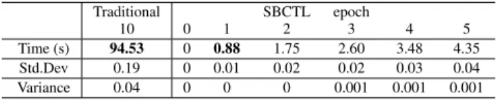
The average training time is shown in Table 5. Overall, in experiment two, SBCTL (initialization B, Euclidean dis-tance) with one epoch achieved 0.55% reduction in MAPE and 474.88 in MAE compared to traditional ML while taking less then 1% of time.
D. EXPERIMENT THREE
This experiment was performed on a machine with Intel i7-9800X processor, 32 GB RAM, and four NVIDIA GeForce
TABLE 5: Experiment 2: Average Training Time
Traditional SBCTL epoch
10 0 1 2 3 4 5
Time (s) 94.53 0 0.88 1.75 2.60 3.48 4.35 Std.Dev 0.19 0 0.01 0.02 0.02 0.03 0.04 Variance 0.04 0 0 0 0.001 0.001 0.001
RTX 2080 Ti graphics cards. As in experiment two, GPU acceleration was used for training machine learning models.
1) Data set
An open source data set provided by the Building Data Genome project [35] was used in this experiment. This data set contains one year of hourly, whole building electrical me-ter data for 507 non-residential buildings. Meme-ters with miss-ing data and with less than one year of data were removed resulting in a set of 456 meters. For each meter there are 24(hours) * 365(days) = 8760 readings. Data were collected between 2010 and 2015 and, as data for each building spans only one year, the collection time periods vary among build-ings. The meters are located in 9 different time zones and there are five primary use types: office, primary/secondary classroom, college laboratory, college classroom, and dormi-tory.
2) Experiment
The challenge with this data set is that it contains only one year of data and for SBCTL ideally, data set should have at least one year for training and additional data for testing. Nevertheless, the last 20% of data was used for testing and the first 80% for training prediction models and for calculating similarities. It is expected that this will not result in as high accuracy as if the hole year of data was used for training.
While in experiments one and two, accuracy could be visualized and observed for each meter separately (as in figures 6 and 10), this is more difficult for experiment three as it contains 456 meters. Thus, traditional machine learning
FIGURE 9: Experiment 2: Test set MAPE at first and fifth epoch.
FIGURE 10: Experiment 2: Test set MAPE for SBCTL and traditional ML.
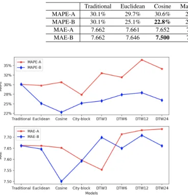
TABLE 6: Experiment 3: MAPE and MAE for initializations A and B, for each distance metrics
Traditional Euclidean Cosine Manhattan DTW3 DTW 6 DTW12 DTW24 MAPE-A 30.1% 29.7% 30.6% 27.4% 33.0% 31.9% 36.5% 34.1% MAPE-B 30.1% 25.1% 22.8% 25.2% 25.8% 27.4% 27.9% 25.9% MAE-A 7.662 7.661 7.652 7.596 7.553 7.714 7.732 7.737 MAE-B 7.662 7.646 7.500 7.593 7.699 7.650 7.709 7.661
FIGURE 11: Experiment 3: MAPE and MAE for different initializations and distance metrics.
was performed with up to 30 epochs with early stopping when the loss function did not decrease in five consecutive epochs. This allows more epochs to achieve convergence, and, at the same time, helps remedy overfitting and avoids higher number of epochs if convergence is achieved earlier.
3) Result
In this experiment, transfer paths were different for the two initialization approachesAandB. Fig. 11 compares MAPE and MAE achieved with the two initializations for each of the distance metrics. The traditional approach does not have different initializations, thus accuracy for initializations A and B is the same. In terms of MAPE, initialization B outperformed initialization A for all distance metrics. This is slightly different for the MAE, where the initializationA achieved better accuracy for DTW with window of 3 time steps (DTW3). Nevertheless, irrelevant of the metrics used, the overall best model is with initialization B and Cosine distance.
Table 6 shows the data from Fig. 11 for further com-parison. It can be observed that the best SBCTL model (initializationBwith Cosine) achieved reduction of 7.3% in average MAPE and .163 in average MAE in comparison to traditional ML training.
The average elapsed time for all meters with the traditional ML and SBCTL are shown in Table 7. SBCTL used only about 2.6% of time needed to train the models in a traditional way.
TABLE 7: Experiment 3: Average Training Time
Traditional SBCTL epoch 10 0 1 2 3 4 5 Time (s) 30.33 0 0.16 0.31 0.46 0.62 0.77 Std.Dev 10.24 0 0.01 0.03 0.04 0.05 0.06 Variance 104.78 0 0 0.001 0.002 0.003 0.004 E. DISCUSSION
In all three experiments, SBCTL achieved improved average accuracy in comparison to traditional ML. Overall, the best performing model was SBTCL with initialization B (from the center) and Euclidean distance. This can be observed from figures 8 and 11 for experiments one and two, whereas there was no difference among SBCTL approaches in the experiment one.
In experiments one and two, SBCTL models trained for 5 epoch achieved higher accuracy than traditional ML with 10 epoch. An exception was meter 4 in experiment two; nevertheless, that meter achieved low accuracy irrelevant of the approach, possibly because of high data variability. This demonstrated that transferring weights according to SBCTL approach is a promising direction for training a large number of energy forecasting models.
Note that in experiment two SBCTL needed only 1 epoch to achieve comparable results to traditional ML where it needed 3 epochs in experiment one. Moreover, in experiment two, even direct transfer without additional training (epoch 0) achieved good accuracy. The reason for this is a higher similarity between meters in experiment two. In experiment one, the lowest Euclidean distance was 135.2 (Table 2) and the mean was 182.65. Meanwhile, the lowest Euclidean distance in experiment two was 0.001 (Table 4) and mean was 34.58.
In all experiments, the time to train SBCTL models was only a fraction of time in comparison to traditional ML while they achieved comparable accuracy. Training time reduction depends on the number of epoch needed after the transfer what is impacted by the similarity between meters.
SBTCL requires all smart meter data sets to have the same sampling frequency or the data sets need to be pre-processed to convert them to the same frequency. If there are any missing data, they need to be imputed in the preparation step in order to enable the similarity calculations. As SBCTL transfers NN weights from one meter to another, and contin-ues training from those weight, there is a possibility of the transferred model getting stuck in a local minimum. How-ever, the presented experiments, even the third one with 456 meters, demonstrate high accuracy in spite of a possibility of
a local minimum.
VI. CONCLUSION
Extensive smart meter deployments have created opportuni-ties for energy forecasting on a large scale. Machine learning-based forecasting typically involves training the model with historical data from a single building and then using this model to infer consumption for the same building. As train-ing is computationally intensive, it is not practical to train ML models individually for many meters.
This paper proposes Similarity-Based Chained Transfer Learning (SBCTL) to enable building neural network-based forecasting models for a large number of smart meters. The initial model is built in a traditional way whereas all other models use transfer learning in a chain-like manner. SBCTL is evaluated with three different data sets: in all experiments, SBCTL achieves similar accuracy to traditional ML training while taking only a fraction of time. The best results are achieved with Euclidean distance and starting from the meter closest to the center. As illustrated in experiments one and two, the SBCTL time depends on the number of epochs needed for convergence after the transfer. When meters are more similar in terms of their energy consumption profiles, SBCTL needs fewer epochs and thus, training time is shorter. The third experiment demonstrates that SBCTL maintains its high accuracy even with a data set of 456 meters.
Future work will further explore the impact of similarly on the number of epochs needed after the transfer. Moreover, possibility to transfer knowledge among data sets of different duration and with different reading intervals will also be explored.
REFERENCES
[1] Y. Wang, Q. Chen, T. Hong, and C. Kang, “Review of smart meter data an-alytics: Applications, methodologies, and challenges,” IEEE Transactions on Smart Grid, 2018.
[2] X. Huang, S. H. Hong, and Y. Li, “Hour-ahead price based energy man-agement scheme for industrial facilities,” IEEE Transactions on Industrial Informatics, vol. 13, no. 6, pp. 2886–2898, 2017.
[3] D. Alahakoon and X. Yu, “Smart electricity meter data intelligence for future energy systems: A survey,” IEEE Transactions on Industrial Infor-matics, vol. 12, no. 1, pp. 425–436, 2016.
[4] K. Amber, R. Ahmad, M. Aslam, A. Kousar, M. Usman, and M. Khan, “In-telligent techniques for forecasting electricity consumption of buildings,” Energy, vol. 157, pp. 886–893, 2018.
[5] K. Hassanpouri Baesmat and A. Shiri, “A new combined method for future energy forecasting in electrical networks,” International Transactions on Electrical Energy Systems, vol. 29, no. 3, p. e2749, 2019.
[6] K. Grolinger, M. A. Capretz, and L. Seewald, “Energy consumption prediction with big data: Balancing prediction accuracy and computational resources,” in 2016 IEEE International Congress on Big Data, pp. 157– 164, 2016.
[7] L. Sehovac, C. Nesen, and K. Grolinger, “Forecasting building energy consumption with deep learning: A sequence to sequence approach,” in IEEE International Congress on Internet of Things, 2019.
[8] S. J. Pan and Q. Yang, “A survey on transfer learning,” IEEE Transactions on knowledge and data engineering, vol. 22, no. 10, pp. 1345–1359, 2010. [9] I. Goodfellow, Y. Bengio, and A. Courville, Deep Learning. MIT Press,
2016. http://www.deeplearningbook.org.
[10] S. Bouktif, A. Fiaz, A. Ouni, and M. Serhani, “Optimal deep learning LSTM model for electric load forecasting using feature selection and genetic algorithm: Comparison with machine learning approaches,” En-ergies, vol. 11, no. 7, p. 1636, 2018.
[11] K. Cho, B. Van Merriënboer, C. Gulcehre, D. Bahdanau, F. Bougares, H. Schwenk, and Y. Bengio, “Learning phrase representations using RNN encoder-decoder for statistical machine translation,” arXiv preprint arXiv:1406.1078, 2014.
[12] L. Tang, X. Wang, X. Wang, C. Shao, S. Liu, and S. Tian, “Long-term electricity consumption forecasting based on expert prediction and fuzzy bayesian theory,” Energy, vol. 167, pp. 1144–1154, 2019.
[13] K. Grolinger, A. L’Heureux, M. A. Capretz, and L. Seewald, “Energy forecasting for event venues: Big data and prediction accuracy,” Energy and Buildings, vol. 112, pp. 222–233, 2016.
[14] Y. Ma, P. Liu, Y. Cui, and S. Liu, “Proposed model employing ARIMA and RELM in urban energy consumption prediction,” in 2018 International Symposium on Computer, Consumer and Control, pp. 465–468, 2018. [15] K. Li, X. Xie, W. Xue, X. Dai, X. Chen, and X. Yang, “A hybrid
teaching-learning artificial neural network for building electrical energy consumption prediction,” Energy and Buildings, vol. 174, pp. 323–334, 2018.
[16] M. Khairalla, X. Ning, N. AL-Jallad, and M. El-Faroug, “Short-term fore-casting for energy consumption through stacking heterogeneous ensemble learning model,” Energies, vol. 11, no. 6, p. 1605, 2018.
[17] S. Han, Y.-h. Qiao, J. Yan, Y.-q. Liu, L. Li, and Z. Wang, “Mid-to-long term wind and photovoltaic power generation prediction based on copula function and long short term memory network,” Applied Energy, vol. 239, pp. 181–191, 2019.
[18] R. Jiao, T. Zhang, Y. Jiang, and H. He, “Short-term non-residential load forecasting based on multiple sequences LSTM recurrent neural network,” IEEE Access, vol. 6, pp. 59438–59448, 2018.
[19] D. L. Marino, K. Amarasinghe, and M. Manic, “Building energy load forecasting using deep neural networks,” in 42nd Annual Conference of the IEEE Industrial Electronics Society, pp. 7046–7051, 2016.
[20] F. Zhu and L. Shao, “Weakly-supervised cross-domain dictionary learning for visual recognition,” International Journal of Computer Vision, vol. 109, no. 1-2, pp. 42–59, 2014.
[21] W. Hu, Y. Qian, F. K. Soong, and Y. Wang, “Improved mispronunciation detection with deep neural network trained acoustic models and transfer learning based logistic regression classifiers,” Speech Communication, vol. 67, pp. 154–166, 2015.
[22] Y. Ma, G. Luo, X. Zeng, and A. Chen, “Transfer learning for cross-company software defect prediction,” Information and Software Technol-ogy, vol. 54, no. 3, pp. 248–256, 2012.
[23] J. Nam, S. J. Pan, and S. Kim, “Transfer defect learning,” in 35th Interna-tional Conference on Software Engineering, pp. 382–391, 2013. [24] W. Li, L. Duan, D. Xu, and I. W. Tsang, “Learning with augmented
features for supervised and semi-supervised heterogeneous domain adap-tation,” IEEE transactions on pattern analysis and machine intelligence, vol. 36, no. 6, pp. 1134–1148, 2014.
[25] A. S. Mozafari and M. Jamzad, “A SVM-based model-transferring method for heterogeneous domain adaptation,” Pattern Recognition, vol. 56, pp. 142–158, 2016.
[26] A. Krizhevsky, I. Sutskever, and G. E. Hinton, “Imagenet classification with deep convolutional neural networks,” in Advances in neural informa-tion processing systems, pp. 1097–1105, 2012.
[27] A. Menegola, M. Fornaciali, R. Pires, F. V. Bittencourt, S. Avila, and E. Valle, “Knowledge transfer for melanoma screening with deep learn-ing,” in IEEE 14th International Symposium on Biomedical Imaging, pp. 297–300, 2017.
[28] S. Lu, Z. Lu, and Y.-D. Zhang, “Pathological brain detection based on alexnet and transfer learning,” Journal of computational science, vol. 30, pp. 41–47, 2019.
[29] E. Mocanu, P. H. Nguyen, W. L. Kling, and M. Gibescu, “Unsupervised energy prediction in a smart grid context using reinforcement cross-building transfer learning,” Energy and Buildings, vol. 116, pp. 646–655, 2016.
[30] T. Grubinger, G. C. Chasparis, and T. Natschläger, “Generalized online transfer learning for climate control in residential buildings,” Energy and Buildings, vol. 139, pp. 63–71, 2017.
[31] M. Ribeiro, K. Grolinger, H. F. ElYamany, W. A. Higashino, and M. A. Capretz, “Transfer learning with seasonal and trend adjustment for cross-building energy forecasting,” Energy and Buildings, vol. 165, pp. 352–363, 2018.
[32] O. Abedinia, N. Amjady, and H. Zareipour, “A new feature selection technique for load and price forecast of electrical power systems,” IEEE Transactions on Power Systems, vol. 32, no. 1, pp. 62–74, 2017.
[33] Z. Yu, Z. Niu, W. Tang, and Q. Wu, “Deep learning for daily peak load forecasting–a novel gated recurrent neural network combining dynamic time warping,” IEEE Access, vol. 7, pp. 17184–17194, 2019.
[34] Kaggle, “Global Energy Forecasting Competition.” https://www.kaggle.com/c/global-energy-forecasting-competition-2012-load-forecasting/data. Online: accessed May 2019.
[35] C. Miller and F. Meggers, “The building data genome project: An open, public data set from non-residential building electrical meters,” Energy Procedia, vol. 122, pp. 439 – 444, 2017.