Data Visualization and Feature Selection: New Algorithms for Nongaussian Data

Data Visualization and Feature Selection:

New Algorithms for Nongaussian Data

Howard Hua Yang and John Moody Oregon Graduate Institute of Science and Technology

20000 NW, Walker Rd., Beaverton, OR97006, USA [email protected], [email protected], FAX:503 7481406

Abstract

Data visualization and feature selection methods are proposed based on the )oint mutual information and ICA. The visualization methods can find many good 2-D projections for high dimensional data interpretation, which cannot be easily found by the other ex-isting methods. The new variable selection method is found to be better in eliminating redundancy in the inputs than other methods based on simple mutual information. The efficacy of the methods is illustrated on a radar signal analysis problem to find 2-D viewing coordinates for data visualization and to select inputs for a neural network classifier.

Keywords: feature selection, joint mutual information, ICA, vi-sualization, classification.

1 INTRODUCTION

Visualization of input data and feature selection are intimately related. A good feature selection algorithm can identify meaningful coordinate projections for low dimensional data visualization. Conversely, a good visualization technique can sug-gest meaningful features to include in a model.

Input variable selection is the most important step in the model selection process. Given a target variable, a set of input variables can be selected as explanatory variables by some prior knowledge. However, many irrelevant input variables cannot be ruled out by the prior knowledge. Too many input variables irrelevant to the target variable will not only severely complicate the model selection/estimation process but also damage the performance of the final model.

Selecting input variables after model specification is a model-dependent approach[6]. However, these methods can be very slow if the model space is large. To reduce the computational burden in the estimation and selection processes, we need model-independent approaches to select input variables before model specification. One such approach is 6-Test [7]. Other approaches are based on the mutual information (MI) [2, 3,4] which is very effective in evaluating the relevance of each input variable, but it fails to eliminate redundant variables.

selec-tion based on joint mutual informaselec-tion (JMI). The increment from MI to JMI is the conditional MI. Although the conditional MI was used in [4] to show the monotonic property of the MI, it was not used for input selection.

Data visualization is very important for human to understand the structural re-lations among variables in a system. It is also a critical step to eliminate some unrealistic models. We give two methods for data visualization. One is based on the JMI and another is based on Independent Component Analysis (ICA). Both methods perform better than some existing methods such as the methods based on PCA and canonical correlation analysis (CCA) for nongaussian data.

2 Joint mutual information for input/feature selection

Let Y be a target variable and Xi'S are inputs. The relevance of a single input is measured by the MI

I(Xi;Y)

=

K(p(Xj,y)llp(Xi)P(Y))

where

K(pllq)

is the Kullback-Leibler divergence of two probability functions

P

and

q

defined by

K(p(x)llq(x))

=

Lx

p(x)

log~.

The relevance of a set of inputs is defined by the joint mutual information

I(Xi'

...

, Xk; Y)

=

K(P(Xi' ... , Xk,

y)llp(Xi' ... ,

Xk)P(Y))·

Given two selected inputs

Xj

and

Xk,

the conditional MI is defined by

I(Xi;

YIXj,

Xk)

=

L

p(Xj, xk)K(p(Xi' ylxj, xk)llp(xilxj, xk)p(ylxj, Xk)).

Similarly define

I(Xi;

YIXj, ... ,

_{X k)}

conditioned on more than two variables.

The conditional MI is always non-negative since it is a weighted average of the Kullback-Leibler divergence. It has the following property

I(XI.

·

··,

X n- l ,

Xn;

Y) -

I(XI ,···,

X n- l ; Y) =

I(Xn;

YIXI ,···, Xn-I)

2:

o.

Therefore,

I(X I ,

···

, X n- l

,

Xn;

Y)

2:

I(X

I ,···, X n- l ;

Y),

i.e., adding the variable

Xn will always increase the mutual information. The information gained by adding a variable is measured by the conditional MI.

When Xn and Yare conditionally independent given Xl,···, Xn - l , the conditional

MI between Xn and Y is

(1)

so Xn provides no extra information about Y when Xl,·· ·,Xn - l are known. In

particular, when Xn is a function of Xl, ... , Xn- l , the equality (1) holds. This is the reason why the joint MI can be used to eliminate redundant inputs.

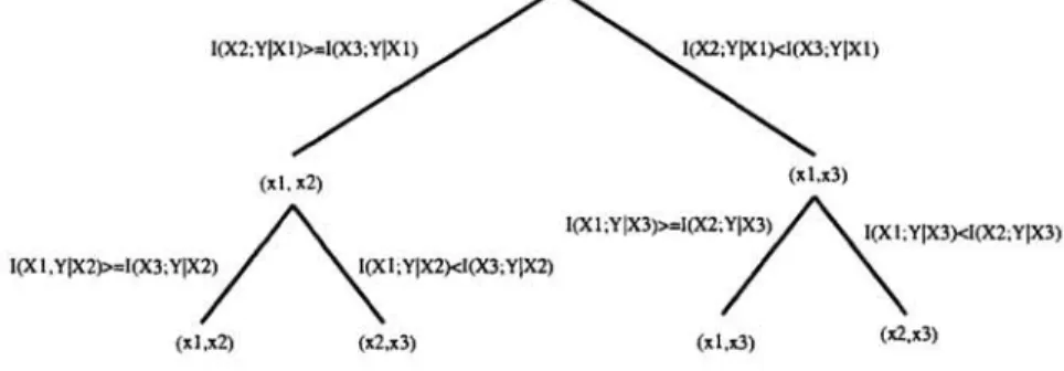
The conditional MI is useful when the input variables cannot be distinguished by the mutual information

I(Xi;Y).

For example, assume

I(XI;Y)

=

I(X2;Y)

I(X3; Y),

and the problem is to select (Xl,

X2),

(Xl,

X3)

or

(X2' X3)

.

Since

I(XI,X2;Y) - I(XI,X3;Y)

=

I(X2;YIXI) - I(X3;YIXt},

we should choose

(Xl, X2)

rather than (Xl,

X3)

if

I(X2;

YIXI )

> I(X3;

YIXI ). Oth-erwise, we should choose (Xl,

X3).

All possible comparisons are represented by a binary tree in Figure 1.

To estimate

I(X

I, ... ,

Xk; Y),

we need to estimate the joint probability

P(XI,··

·,

Xk, y).

This suffers from the curse of dimensionality when k is large.

Data Visualization and Feature Selection 689

Sometimes, we may not be able to estimate high dimensional MI due to the sample

shortage. Further work is needed to estimate high dimensional joint MI based on

parametric and non-parametric density estimations, when the sample size is not

large enough.

In some real world problems such as mining large data bases and radar pulse classi-fication, the sample size is large. Since the parametric densities for the underlying distributions are unknown, it is better to use non-parametric methods such as his-tograms to estimate the joint probability and the joint MI to avoid the risk of specifying a wrong or too complicated model for the true density function.

(xl. x2) (xl.x3)

"'

A.

.~

l(Xl;Y\X3»:1(X2;Y\X3y\!(XLY\X3)<1(X2;Y\X3)

1(Xl.Y\X2»:1(X3;Y\X/, , \ 1;Y\X2l<1(X3;Y\X2) / " \

(xl.x2) (x2.x3) (x1.xl) (xl,x3)

Figure 1: Input selection based on the conditional MI.

In this paper, we use the joint mutual information I(Xi, Xj; Y) instead of the

mutual information I(Xi; Y) to select inputs for a neural network classifier. Another

application is to select two inputs most relevant to the target variable for data visualiz ation.

3

Data visualization methods

We present supervised data visualization methods based on joint MI and discuss unsupervised methods based on ICA.

The most natural way to visualize high-dimensional input patterns is to dis-play them using two of the existing coordinates, where each coordinate corre-sponds to one input variable. Those inputs which are most relevant to the

tar-get variable corresponds the best coordinates for data visualization, Let (i*, j*)

=

arg maxU,nI(Xi, Xj; Y). Then, the coordinate axes (Xi-, Xj-) should be used for visualizing the input patterns since the corresponding inputs achieve the maximum

joint MI. To find the maximum I(Xj-, Xj-IY), we need to evaluate every joint MI

I(Xi' Xj; Y) for i

<

j. The number of evaluations is O(n2 ).

Noticing that I(Xj,Xj;Y)

=

I(Xi;Y)

+

I(Xj;YIXi), we can first maximize the

MI I(Xi; Y), then maximize the conditional MI. This algorithm is suboptimal, but

only requires n - 1 evaluations of the joint MIs. Sometimes, this is equivalent to

exhaustive search. One such example is given in next section.

Some existing methods to visualize high-dimensional patterns are based on dimen-sionality reduction methods such as PCA and CCA to find the new coordinates to

display the data, The new coordinates found by PCA and CCA are orthogonal in

Euclidean space and the space with Mahalanobis inner product, respectively. How-ever, these two methods are not suitable for visualizing nongaussian data because the projections on the PCA or CCA coordinates are not statistically independent

for nongaussian vectors. Since the JMI method is model-independent, it is better

Both CCA and maximumjoint MI are supervised methods while the PCA method

is unsupervised. An alternative to these methods is ICA for visualizing clusters [5].

The ICA is a technique to transform a set of variables into a new set of variables,

so that statistical dependency among the transformed variables is minimized. The

version of ICA that we use here is based on the algorithms in [1, 8]. It discovers

a non-orthogonal basis that minimizes mutual information between projections on

basis vectors. We shall compare these methods in a real world application.

4

Application to Signal Visualization and Classification

4.1 Joint mutual information and visualization of radar pulse patterns

Our goal is to design a classifier for radar pulse recognition. Each radar pulse

pattern is a 15-dimensional vector. We first compute the joint MIs, then use them

to select inputs for the visualization and classification of radar pulse patterns.

A set of radar pulse patterns is denoted by D = {(zi, yi) : i = 1"", N} which

consists of patterns in three different classes. Here, each Zi E

R

t5 _{and each yi E}

{I, 2, 3}. , 14 I~

"

MIl"" mlormabon 0 CondIIionai NI given X2 2 12 1 i e-::E 0.8 J

1

~ 106 to 8 I ;; t>: 0.' , t> I> 02 ~ I> 0 0 0 _~.'.a .. ,. 0 0 0 0 " .~::: 0 I> .. 00 '0 15 02 0

1J

J

11

1 2 3 .4 5 6 7 8 9 10 11 12 13 14 15

Inputvanablallldex bundle nutrtJer

(a) (b)

Figure 2: (a) MI vs conditional MI for the radar pulse data; maximizing the MI then

the conditional MI with O(n) evaluations gives I(Xil' Xii; Y) = 1.201 bits. (b) The

joint MI for the radar pulse data; maximizing the joint MI gives I(Xi. ,Xj-; Y)

=

1.201 bits with O(n2 ) evaluations of the joint MI. (il'

it)

=

(i*, j*) in this case.

Let it = arg maxJ(Xi;Y) and

it

= arg maXj;tiJ(Xj;YIXi1 ). From Figure 2(a),

we obtain (it,it)

=

(2,9) and I(XillXjl;Y) = I(Xil;Y)

+

I(Xj1;YIXi1 )

=

1.201 bits. If the number of total inputs is n, then the number of evaluations for

computing the mutual information I(Xi; Y) and the conditional mutual information

I(Xj; YIXiJ is O(n).

To find the maximum I(Xi-, X j>; Y), we evaluate every I(Xi, Xj; Y) for i

<

j.

These MIs are shown by the bars in Figure 2(b), where the i-th bundle displays the MIs I(Xi,Xj;Y) for j

=

i+

1" " ,15.

In order to compute the joint MIs, the MI and the conditional MI is evaluated 0 (n)

and O(n2 ) times respectively. The maximumjoint MI is I(Xi-, X j -; Y) = 1.201 bits.

Data Visualization and Feature Selection 691

application, the equality holds. This suggests that sometimes we can use an efficient

algorithm with only linear complexity to find the optimal coordinate axis view

(Xi·,Xj.). The joint MI also gives other good sets of coordinate axis views with

high joint MI values.

3.~

2 0 0 N '"

'I"llll~

c . ~ 0 ~ ~o 3 3 ~ 33 8 .,

..

_!O <> _x .~ ~ 0 Ii ' /2

h

0 '" 'l' ~ ·20 -,0 ,0 20 -20 20 40

firs, prinopol oomponen' X2

(a) (b) 25 J 3 ₃ 3J3 3 15 ₁ 1 1 ~, 3 3 1 1 1 N " f 1 _• §~~ 3 1

,

"

,

'

1 1 1

.

~j;l;,

1

1~~1

~

~

, 3 1 ₁ Cl

,

• 1 ..J 05 /20

,

~,

,

3 3 3 3 § , " , 3 f 2 3 3 3 3 3 3 0

,

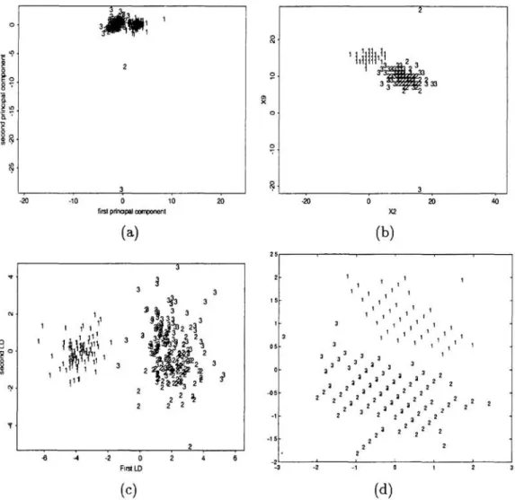
" _" 2 a> 3 3 3 3 ₂ 1,1 2~:ai 2~ ~ 3 3 3 3 3 3 3 3 2 2 2 'l' 2 2 3 ₂ 2 ₃ 3 ₂ 2 2 2 ~ -<15 2 ₂ 2 2 ₂ 3 3 ₂ 2 2 ₂ 2 2 3 ₂ 3 ₃ 2 ₂ 2 3 2 2 3 3 ₂ 2 -1 2 2 _{2 3} 2 2 '1 ₃ 2 ₂ 2 2 2 -15 ₂ 2 -6 ~ ·2 _-2 2 F.rstLD -3 -2 -1 (c) (d)

Figure 3: (a) Data visualization by two principal components; the spatial relation

between patterns is not clear. (b) Use the optimal coordinate axis view (Xi., Xj-)

found via joint MI to project the radar pulse data; the patterns are well spread

to give a better view on the spatial relation between patterns and the boundary

between classes. (c) The CCA method. (d) The ICA method.

Each bar in Figure 2(b) is associated with a pair of inputs. Those pairs with high

joint MI give good coordinate axis view for data visualization. Figure 3 shows that

the data visualizations by the maximum JMI and the ICA is better than those by

the PCA and the CCA because the data is nongaussian.

4.2 Radar pulse classification

Now we train a two layer feed-forward network to classify the radar pulse patterns.

Figure 3 shows that it is very difficult to separate the patterns by using just two

into a training set DI and a test set D2 consisting of 20 percent patterns in D. The

network trained on the data set DI using all input variables is denoted by

Y = f(XI ,'" ,Xn; WI, W 2 , 0)

where WI and W 2 are weight matrices and 0 is a vector of thresholds for the hidden

layer.

From the data set D, we estimate the mutual information I(Xi; Y) and select

il

=

arg maxJ(Xi ; Y). Given Xii' we estimate the conditional mutual information

I(Xj; YIXii ) for j =1= il . Choose three inputs Xi'J' Xi3 and Xi 4 with the largest

conditional MI. We found a quartet (iI, i2, i3, i4)

=

(1,2,3,9). The two-layer

feed-forward network trained on DI with four selected inputs is denoted by

Y

=

g(XI,X2 , X3 , X g; W~, W~, 0').

There are 1365 choices to select 4 input variables out of 15. To set a reference

perfor-mance for network with four inputs for comparison. Choose 20 quartets from the set

Q

=

{(h,h,h,h):

1 ~ jl

<

h

<

h

<

j4

~ 15}. For each quartet

(h,h,h,j4),

a

two-layer feed-forward network is trained using inputs (XjllXh,Xh,Xj4)' These

networks are denoted by

Y

=

hi(Xil ,Xh , Xh, X j4 ; W~, W~, 0"), i

=

1,2"",20 .

•

•

.

.

.55 - . . . . w..q ER. wlh3)QJnIIa

I

- -- . . . . ~ER 'd\mcpdltl - -. If'1n11ER lIIIII'I4I1111d1dtnpilXl.X2,l(3,n:G

1>---+ 1eItIngst.., 4.-..ct .... XI, X2.)(J, MIl xv

nini'I EA .. . . Xl,X2, lQ,_)fJ ... ER; . . . Xl.X2.lQ .... XI ... a. . .., .. ~ ... Eft ... ...,. 5

...

• ,

-

_~

-

-

_{- -}

--

-

-3 l\ I I 015 .25

\~

2 I \ . ' , 5 " \ . , Y , , '7;:Y.-1 .... ... -'.1

••

10 15 25

--

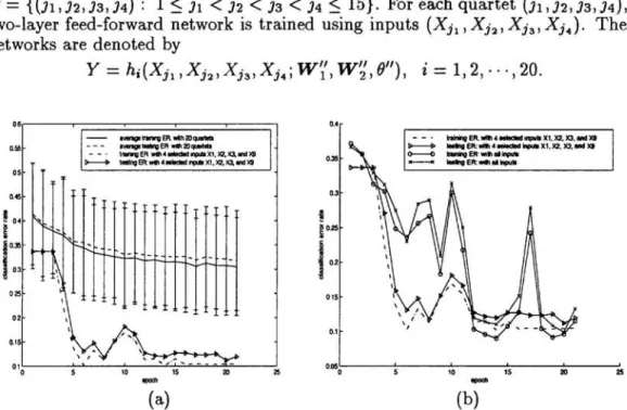
(a) (b)

-Figure 4: (a) The error rates of the network with four inputs (Xl, X2 , X3 , Xg)

selected by the joint MI are well below the average error rates (with error bars

attached) of the 20 networks with different input quartets randomly selected; this

shows that the input quartet (XI ,X2,X3,X9 ) is rare but informative. (b) The

network with the inputs (XI,X2,X3,X9 ) converges faster than the network with

all inputs. The former uses 65% fewer parameters (weights and thresholds) and

73% fewer inputs than the latter. The classifier with the four best inputs is less

expensive to construct and use, in terms of data acquisition costs, training time,

and computing costs for real-time application.

The mean and the variance of the error rates of the 20 networks are then computed.

All networks have seven hidden units. The training and testing error rates of the

networks at each epoch are shown in Figure 4, where we see that the network

with four inputs selected by the joint MI performs better than the networks with

randomly selected input quartets and converges faster than the network with all

inputs. The network with fewer inputs is not only faster in computing but also less

Data Visualization and Feature Selection 693

5

CONCLUSIONS

We have proposed data visualization and feature selection methods based on the

joint mutual information and ICA.

The maximum JMI method can find many good 2-D projections for visualizing high

dimensional data which cannot be easily found by the other existing methods. Both

the maximum JMI method and the ICA method are very effective for visualizing nongaussian data.

The variable selection method based on the JMI is found to be better in eliminating

redundancy in the inputs than other methods based on simple mutual information. Input selection methods based on mutual information (MI) have been useful in many applications, but they have two disadvantages. First, they cannot distinguish inputs when all of them have the same MI. Second, they cannot eliminate the redundancy in the inputs when one input is a function of other inputs. In contrast, our new

input selection method based on th~ joint MI offers significant advantages in these

two aspects.

We have successfully applied these methods to visualize radar patterns and to select

inputs for a neural network classifier to recognize radar pulses. We found a smaller

yet more robust neural network for radar signal analysis using the JMI.

Acknowledgement: This research was supported by grant ONR

N00014-96-1-0476.

References

[1] S. Amari, A. Cichocki, and H. H. Yang. A new learning algorithm for blind

signal separation. In Advances in Neural Information Processing Systems, 8,

eds. David S. Touretzky, Michael C. Mozer and Michael E. Hasselmo, MIT

Press: Cambridge, MA., pages 757-763, 1996.

[2] G. Barrows and J. Sciortino. A mutual information measure for feature selection with application to pulse classification. In IEEE Intern. Symposium on

Time-Frequency and Time-Scale Analysis, pages 249-253, 1996.

[3] R. Battiti. Using mutual information for selecting features in supervised neural

net learning. IEEE Trans. on Neural Networks, 5(4):537-550, July 1994. [4] B. Bonnlander. Nonparametric selection of input variables for connectionist

learning. Technical report, PhD Thesis. University of Colorado, 1996.

[5] C. Jutten and J. Herault. Blind separation of sources, part i: An adaptive

algorithm based on neuromimetic architecture. Signal Processing, 24:1-10, 1991. [6] J. Moody. Prediction risk and architecture selection for neural network. In V. Cherkassky, J .H. Friedman, and H. Wechsler, editors, From Statistics to

Neural Networks: Theory and Pattern Recognition Applications. NATO ASI

Series F, Springer-Verlag, 1994.

[7] H. Pi and C. Peterson. Finding the embedding dimension and variable depen-dencies in time series. Neural Computation, 6:509-520, 1994.

[8] H. H. Yang and S. Amari. Adaptive on-line learning algorithms for blind

sep-aration: Maximum entropy and minimum mutual information. Neural