BDDs for Pseudo-Boolean Constraints

Constraints – Revisited

Ignasi Ab´ıo, Robert Nieuwenhuis, Albert Oliveras,

and Enric Rodr´ıguez-Carbonell

Technical University of Catalonia (UPC), Barcelona

Abstract. Pseudo-Boolean constraints are omnipresent in practical applications, and therefore a significant effort has been devoted to the development of good SAT encoding techniques for these constraints. Sev-eral of these encodings are based on building Binary Decision Diagrams (BDDs) and translating these into CNF. Indeed, BDD-based encodings have important advantages, such as sharing the same BDD for repre-senting many constraints.

Here we first prove that, unless NP = Co-NP, there are Pseudo-Boolean constraints that admit no variable ordering giving a polyno-mial (Reduced, Ordered) BDD. As far as we know, this result is new (in spite of some misleading information in the literature). It gives several interesting insights, also relating proof complexity and BDDs.

But, more interestingly for practice, here we also show how to over-come this theoretical limitation bycoefficient decomposition. This allows us to give the first polynomial arc-consistent BDD-based encoding for Pseudo-Boolean constraints.

1

Introduction

In this paper we study Pseudo-Boolean constraints (PB constraints for short), that is, constraints of the form_a1x1+· · ·+anxn#K, where theai andK are

integer coefficients, the_xi are Boolean (0/1) variables, and the relation operator # belongs to{<, >,≤,≥,=}. We will assume that # is≤and the_ai and_K are positive since other cases can be easily reduced to this one (see [ES06]).

Such a constraint is a Boolean function_C:{0_,1}n→ {0_,1}that is monotonic decreasing in the sense that any solution for_C remains a solution after flipping inputs from 1 to 0. Therefore these constraints can be expressed by a set of clauses with only negative literals. For example, each clause could simply define a (minimal) subset of variables that cannot be simultaneously true. Note however that not every such a monotonic function is a PB constraint. For example, the function expressed by the two clauses_x1∨x2andx3∨x4has no (single) equivalent

PB constraint_a1x1+· · ·+anxn ≤K(since wlog.a1≥a2anda3≥a4, and then

_{All the authors are partially supported by Spanish Min. of Educ. and Science through}

the LogicTools-2 project (TIN2007-68093-C02-01). Ab´ıo is also partially supported by FPU grant.

K.A. Sakallah and L. Simon (Eds.): SAT 2011, LNCS 6695, pp. 61–75, 2011. c

also _x1∨x3 is needed). Hence, even among the monotonic Boolean functions,

PB constraints are a rather restricted class (see also [J.S07]).

PB constraints are omnipresent in practical SAT applications, not just in typ-ical 0-1 linear integer problems, but also as an ingredient in new SAT approaches to, e.g., cumulative scheduling [SFSW09], so it is not surprising that a signifi-cant number of SAT encodings for these constraints have been proposed in the literature. Here we are interested in encoding a PB constraint_Cby a clause set

S (possibly with auxiliary variables) that is not only equisatisfiable, but also (generalized)arc-consistent: given a partial assignment_A, if_xi is false in every extension of_Asatisfying_C, then unit propagating_Aon_S sets_xi to false.

To our knowledge, the only polynomial arc-consistent encoding so far was given by Bailleux, Boufkhad and Roussel [BBR09]. Other existing encodings are based on building (forms of) Binary Decision Diagrams (BDDs) and translating these into CNF. Although [BBR09] is not BDD-based, our motivation to revisit BDD-based encodings is twofold:

Example 1. Consider the constraint 3_x1 + 2x2+ 4x3 ≤ 5 and the constraint

30001_x1+ 19999x2+ 39998x3≤50007. Both are clearly equivalent: the Boolean

function they represent can be expressed, e.g., by the clauses_x1∨x3andx2∨x3.

However, encodings like the one of [BBR09] heavily depend on the concrete co-efficients of each constraint, and generate a significantly larger SAT encoding for the second one. Since, given a variable ordering, (Reduced, Ordered) BDDs are a canonical representation for Boolean functions [Bry86], i.e., each Boolean function has a unique ROBDD, a ROBDD-based encoding will treat both

con-straints equivalently.

The second reason for revisiting BDDs is that in practical problems numerous PB constraints exist that share variables among each other. Representing them all as a single BDD has the potential of generating a much more compact SAT encoding that is moreover likely to have better propagation properties.

Related work. The same authors of [BBR09] proposed an encoding “very close to those using a BDD and translating it into clauses” [BBR06]. It is arc-consistent, but an example of a PB constraint family is given in [BBR06] for which their kind of non-reduced BDDs, with their concrete variable order-ing is exponentially large. However, as we show here, ROBDDs for this fam-ily are polynomial. Their method works as follows. Given the PB constraint

a1x1+· · ·+a_nx_n ≤ K with coefficients ordered from small to large, the root

node is labelled with variable_Dn,K, expressing that the sum of the first_nterms is no more than _K. Its two children are _Dn−1,K and Dn−1,K−a_n, which

cor-respond to setting _xn to false and true, respectively, etc. Two binary and two ternary clauses per node express the relationships between the variables.

Example 2. The encoding of [BBR06] on 2_x1+· · ·+ 2x10+ 5x11+ 6x12≤10 is

illustrated in Figure 1. Node_D10,5represents 2x1+ 2x2+· · ·2x10≤5, whereas

node_D10,4represents 2x1+ 2x2+· · ·2x10≤4. The method fails to identify that

both these PB constraints are equivalent and hence subtrees_B and _C will not be merged, yielding a much larger representation than with ROBDDs.

D12,10 D11,10 D11,4 D10,10 D10,5 D10,4 D_≡10_false,−1 0 0 0 1 1 1 A B C

Fig. 1.Tree-like construction of [BBR06] for 2x1+· · ·+ 2x10+ 5x11+ 6x12≤10

On the other hand, E´en and S¨orensson use ROBDDs in MiniSAT+ [ES06]. Their encoding uses six three-literal clauses per BDD node and is arc-consistent, but the proof of arc-consistency relies on a particular variable ordering. Regarding the size of their ROBDDs, they cite [BBR06] to say“It is proven that in general a PB-constraint can generate an exponentially sized BDD [BBR06]” which, as we have seen, cannot be concluded from that paper since they do not use ROB-DDs. Apart from their BDD-based encoding, [ES06] also suggests two alternative methods: one based on adder networks (O(_n) in size but not arc-consistent) and another one based on sorting networks (O(_nlog_n) in size and not arc-consistent). Finally, as we have already mentioned, [BBR09] presents an arc-consistent and polynomial BDD-based SAT encoding (sizeO(_n2_log

nlog_amax), i.e., it de-pends on the size of the coefficients) based on a network of unary adders. Main Contributions and Organization of This Paper

• Subsection 3.2: The first, to our knowledge, PB constraint family for which ROBDDs with small-to-large variable ordering are exponential in size (and also for the large-to-small ordering).

• Subsection 3.3: A proof that, unless NP=co-NP, there are PB constraints that admit no polynomial-size ROBDD, independently of the variable order.

• Subsection 4.1: A proof that PB constraints whose coefficients are powers of two do admit polynomial-size BDDs.

• Subsections 4.2 and 4.3: An arc-consistent and polynomial (size

O(_n3_log

amax)) BDD-based encoding for PB constraints.

• Section 5: An arc-consistent SAT encoding of BDDS for monotonic functions, a more general class of Boolean functions than PB constraints. This encoding uses only one binary and one ternary clause per node (the standard if-then-else encoding for BDDs used in, e.g., [ES06], requires six ternary clauses per node). Moreover, this translation works for any BDD variable ordering.

2

Preliminaries

We assume the reader is familiar with the basic notions of propositional logic. Otherwise, basic definitions can be found in [BHvMW09]. Pseudo-Boolean con-straints (PB concon-straints for short) are concon-straints of the form _a1x1 +· · · +

anxn # _K, where the _ai and _K are integer coefficients, the _xi are Boolean (0/1) variables, and the relation operator # belongs to{<, >,≤,≥,=}. We will assume that # is≤and the_aiand_Kare positive, since other cases can be easily reduced to this one1_{: (i) changing into≤is straightforward if coefficients can be}

negative; (ii) replacing−axby_a(1−_x)−_a; (iii) replacing (1−_x) by_x. Negated variables like_xcan be handled as positive ones or, alternatively, replaced by a fresh_x and adding the clauses_x∨_x and_x∨_x.

Our main goal is to find SAT encodings for PB constraints. That is, given a PB-constraint_C, construct an equisatisfiable clause set (a CNF)_Ssuch that any model for_Srestricted to the variables of_Cis a model of_C. Two extra properties are sought: (i)consistency checking by unit propagation or simply consistency: whenever a partial assignment _A cannot be extended to a model for _C, unit propagation on_S and _A produces a contradiction (a literal_l and its negation

l); and (ii) (generalized)arc-consistency (again by unit propagation): given an assignment _A that can be extended to a model of _C, but such that _A∪ {x} cannot, unit propagation on_S and _A produces_x. More concretely, we will use BDDs for finding such encodings, as illustrated by the following example.

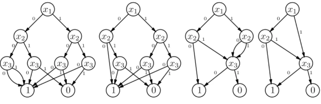
x1 x2 x2 x3 x3 x3 x3 0 1 1 1 1 1 1 1 1 0 0 0 0 0 0 0 x1 x2 x2 x3 x3 x3 0 1 1 1 1 1 1 1 0 0 0 0 0 0 x1 x2 x2 x3 0 1 1 1 1 1 0 0 0 0 x1 x2 x3 0 1 1 1 1 0 0 0

Fig. 2.Construction of a BDD for 2x1+ 3x2+ 5x3≤6

Example 3. Figure 2 explains (one method for) the construction of a ROBDD for the PB constraint 2_x1+ 3x2+ 5x3 ≤ 6 and the ordering x1 < x2 < x3.

The root node has as selector variable _x1. Its false child represents the PB

constraint assuming _x1 = 0 (i.e., 3x2+ 5x3 ≤ 6) and its true child represents

2 + 3_x2+ 5x3 ≤ 6, that is, 3x2+ 5x3 ≤ 4. The two children have the next

variable in the ordering (_x2) as selector, and the process is repeated until we

reach the last variable in the sequence. Then, a constraint of the form 0≤ _K is the True node (1 in the figure) if _K ≥0 is positive, and the False node (0)

1 _{An =-constraint can be split into a≤-constraint and a≥-constraint. Here we}

if _{K <} 0. This construction (leftmost in the figure), is known as an Ordered BDD. For obtaining a Reduced Ordered BDD (BDD for short in the rest of the paper), two reductions are applied until fixpoint: removing nodes with identical children (as done with the leftmost_x3node in the second BDD of the figure), and

merging isomorphic subtrees, as done for_x3 in the third BDD. The fourth final

BDD is a fixpoint. For a given ordering, BDDs are a canonical representation of Boolean functions: each Boolean function has a unique BDD. BDDs can be encoded in CNF by introducing an auxiliary variable _a for every node. If the selector variable of the node is _xand the auxiliary variables for the false and true child are_f and_t, respectively, add the if-then-else clauses:

x∧f →a x∧t→a f ∧t→a

x∧f →a x∧t→a f ∧t→a

In what follows, the size of a BDD is its number of nodes. We will say that a BDD represents a PB constraint if they represent the same Boolean function. Given an assignment_Aover the variables of a BDD, we define thepath induced by_Aas the path that starts at the root of the BDD and at each step, moves to the false (true) child of a node iff its selector variable is false (true) in_A.

3

Exponential BDDs for PB Constraints

In this section, we prove that, unless NP=co-NP, there are PB constraints whose BDDs are all exponential, regardless of the variable ordering. We start by defin-ing the notion of the interval of a PB constraint. After that, we consider two families of PB constraints and we study the size of their BDDs. Finally, we prove the main result of this section.

3.1 Intervals

Example 4. Consider the constraint 2_x1+ 3x2+ 5x3≤6. Since no combination

of its coefficients adds to 6, the constraint is equivalent to 2_x1+ 3x2+ 5x3<6,

and hence to 2_x1+ 3x2+ 5x3≤5. This process cannot be repeated again since 5

can be obtained with the existing coefficients.

Similarly, we could try to increase the right-hand side of the constraint. How-ever, there is a combination of the coefficients that adds 7, which implies that the constraint is not equivalent to 2_x1+ 3x2+ 5x3≤7. All in all, we can state

that the constraint is equivalent to 2_x1+ 3x2+ 5x3≤Kfor anyK∈[5,6]. It is

trivial to see that the set of valid_K’s is always an interval. Definition 1. Let _C be a constraint of the form _a1x1+· · ·+anxn ≤K. The

intervalof _C consists of all integers _M such that _a1x1+· · ·+anxn≤M, seen

as a Boolean function, is equivalent to_C.

In the following, given a BDD representing a PB constraint and a node_ν, we will refer tothe interval of_ν as the interval of the constraint represented by the BDD rooted at _ν. Unless stated otherwise, the ordering used in the BDD will be_x1< x2< . . . < xn.

Proposition 2. If [_{β, γ}] is the interval of a node _ν with selector variable _xi then:

1. There is an assignment {x_j=_vj}n_j=i such that _aivi+· · ·+_anvn=_β.

2. There is an assignment {x_j=_vj}n_j=i such that _aivi+· · ·+_anvn=_γ+ 1_.

3. There is an assignment {x_j = _vj}i_j−₌₁1 such that _K−_a1v1−a2v2− · · · −

ai−1vi−1∈[β, γ]

4. Take_{h < β}. There exists an assignment{x_j =_vj}_jn_=i such that _aivi+· · ·+

anvn > hand its path goes from ν to True.

5. Take_{h > γ}. There exists an assignment{x_j=_vj}_jn_=i such that_aivi+· · ·+

anvn ≤hand its path goes from ν to False.

6. The interval of the True node is [0_,∞).

7. The interval of the False node is(−∞,−1]. Moreover, it is the only interval with negative values.

We now prove that, given a BDD for a PB constraint, one can easily compute the intervals for every node bottom-up. We first start with an example.

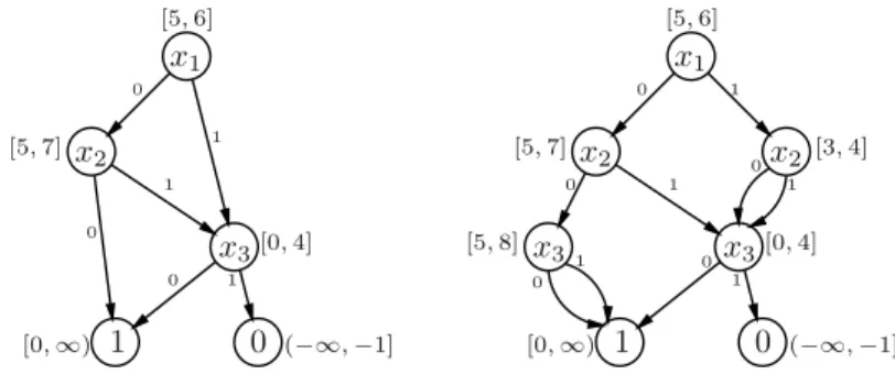
x1 x2 x3 0 1 1 1 1 0 0 0 [5,6] [5,7] [0,4] [0,∞) (−∞,−1] x1 x2 x2 x3 x3 0 1 1 1 1 1 1 0 0 0 0 0 [5,6] [5,7] [3,4] [5,8] [0,4] [0,∞) (−∞,−1]

Fig. 3.Intervals of the BDD for 2x₁+ 3x₂+ 5x₃≤6

Example 5. Let us consider again the constraint 2_x1+ 3x2+ 5x3≤6. Assume

that all variables appear in every path from the root to the leaves (otherwise, add extra nodes as in the rightmost BDD of Figure 3). Assume now that we have computed the intervals for the two children of the root (rightmost BDD in Figure 3). This means that the false child of the root is the BDD for 3_x2+ 5x3≤

[5_,7] and the true child the BDD for 3_x2+ 5x3 ≤ [3,4]. Assuming x1 to be

false, the false child would also represent the constraint 2_x1 + 3x2 + 5x3 ≤

[5_,7], and assuming_x1 to be true, the true child would represent the constraint

2_x1+ 3x2+ 5x3≤[5,6]. Taking the intersection of the two intervals, we can infer

that the root node represents 2_x1+ 3x2+ 5x3≤[5,6].

More formally, the interval of every node can be computed as follows:

Proposition 3. Let_a1x1+a2x2+· · ·+anxn≤K be a constraint, and letB be

xi, false child _νf (with selector variable _xf and interval [_{βf, γf}]) and true child

νt(with selector variable_xtand interval[_{βt, γt}]). The interval of_νis[_{β, γ}], with:

β = max{β_f+_ai+1+· · ·+a_f−1, β_t+a_i+a_i+1+· · ·+a_t−1},

γ= min{γ_{f, γt}+_ai}.

If in every path from the root to the leaves of the BDD all variables were present, the definition of _β would be much simpler (_β = max{β_{f, βt}+_ai}). The other coefficients are necessary to account for the variables that have been removed due to the BDD reduction process.

3.2 Some Families of PB Constraints and Their BDD Size

We start by revisiting the family of PB constraints given in [BBR06], where it is proved that, for their concrete variable ordering, their non-reduced BDDs grow exponentially for this family. Here we prove that ROBDDs are polynomial for this family, and that this is even independent of the variable ordering. The family is defined by considering_a,_band_npositive integers such that n_i=1bi _{< a}. The coefficients are_ωi=_a+_biand the right-hand side of the constraint is_K=a·n/2. We will first prove that the constraint_C:_ω1x1+· · ·+ωnxn ≤K is equivalent

to the cardinality constraint _C : _x1+· · ·+xn ≤n/2−1. For simplicity, we

assume that_nis even.

– Take an assignment satisfying _C. In this case, there are at most_n/2−1 variables_xiassigned to true, and the assignment also satisfies_Csince:_ω1x1+

· · ·+_ωnxn≤ n i=n/2+2 ωn= (n/2−1)a+ n i=n/2+2 bn< K−a+ n i=1 bi< K.

– Consider now an assignment not satisfying _C. In this case, there are at least _n/2 true variables in the assignment and it does not satisfy _C either:

ω1x1+· · ·+ωnxn n/2 i=1 ωi= (_n/2)·_a+ n/2 i=1 bi>(_n/2)·_a=_K.

Since the two constraints are equivalent and BDDs are canonical, the BDD representation of_C and_C are the same. But the BDD of_C is known to be of quadratic size because it is a cardinality constraint (see, for instance, [BBR06]). Theorem 4. There exists a family of PB constraints parameterized by_n, whose ROBDDs grow exponentially in_nwhen ordering the variables according to their coefficients from small to large. The same happens ordering from large to small.

Proof. We consider constraints of the form_a1x1+· · ·+a4nx4n ≤K. It is

2_n a1 = 0 0 0 0 0 · · · 01 = 1 a2 = 0 0 0 0 0 · · · 10 = 2 · · · . .. a2n−1 = 0 0 0 01 · · · 0 0 a2n = 0 0 0 10 · · · 0 0 = 22n−1 a2n+1 = 10 0 0 0 · · · 01 a2n+2 = 10 0 0 0 · · · 10 · · · . .. a4n−1 = 10 0 01 · · · 0 0 a4n = 10 0 10 · · · 0 0 K = _{dm . . . d}00 0 1 1 · · · 1 1

where_{dm. . . d}0 is the binary representation ofn. Note that, to sum to exactly

K, one needs exactly_ncoefficients of the bottom half (between_a2n+1 anda4n)

to obtain the digits_{dm. . . d}0, and that, once such a subset is chosen, a unique

subset of exactly _n coefficients of the top half exists that will complete the 11_{. . .}11 suffix of_K. Reversely, for each subset of size_nof the top half, a unique subset of size_nof the bottom half exists that complements it to sum exactly_K. Now consider a BDD ordered_x1<· · ·< x4n, and any two distinct assignments

T and _T for _x1. . . x2n that set exactly n variables to true. Then T and T

induce paths that necessarily lead to different nodes of the BDD. To see this, wlog., assume that the sum of coefficients corresponding to true variables in _T is smaller than the one of_T. Consider the assignment_Bto_x2_n. . . x4_nthat sets

to true the unique size-_n subset of the bottom half coefficients that sums to_K for _T (and hence exceeds _K for _T). Then the PB constraint satisfies _T ∪_B, but not_T∪_B; hence_B distinguishes the nodes for_T and_T. Altogether, the BDD must have at least as many nodes as distinct assignments setting exactly

n variables of the top half to true, i.e., an exponential number,

2_n

n

. For the large-to-small ordering exactly the same reasoning applies2. For the PB constraint family of the previous proof, it can be shown that the “interleaved” ordering _x1 < x2n+1 < x2 < x2n+2 < . . . < x2n < x4n leads to

a polynomial-sized BDD (the proof is non-trivial, but we had to omit it here due to space limitations). The next natural step would be to present a concrete family of PB constraints whose BDDs are always exponential regardless of the variable ordering. We have not been able to find such a family. But in the next section we prove that, unless NP=co-NP, such a family must exist.

3.3 Probably There Are No Small BDDs for All PB Constraints Our goal is now to prove that, unless NP=co-NP, there are PB constraints all whose BDDs are exponential, independently of the variable ordering. The

main ingredient is an algorithm that, given a BDDB and a PB constraint _C:

a1x1+· · ·+anxn ≤K over the same set of variables, allows one to decide, in

time polynomial in the size of the BDD, whetherBrepresents_C. Again, w.l.o.g., we assume that the BDD ordering is_x1< x2< . . . < xn.

Given the BDD, the algorithm first computes, in a bottom-up manner, an interval for every node of the BDD, as explained in Proposition 3 and points 6 and 7 of Proposition 2. Note that the cost of computing a single interval isO(_n) and hence computing all intervals takesO(_nm) time, where_mis the BDD’s size. After that, we know thatBis a representation of _Cif and only if _K belongs to the interval of the BDD root.

Theorem 5. Bis a BDD representing a PB constraint_a1x1+· · ·+anxn≤Kif,

and only if,_Kbelongs to the interval of the root ofBcomputed by our algorithm. Proof. IfBis a BDD representing_C, then_K belongs to the interval of the root by definition of interval (Def. 1). Moreover, Proposition 3 guarantees that our algorithm correctly computes such an interval.

Let us now assume thatB is not a BDD representing _C. Then, there exists an assignment{x1 =v1, . . . , xn =vn} that either satisfies C but leads to the

False node inBor does not satisfy_C but leads to the True node inB.

Let us assume that the assignment satisfies _C. The other case is analog to this one. In this case, we will prove that_γ1 < K, where [β1, γ1] is the interval

computed for the root node.

We define a sequence of nodes_ν1, ν2, . . . , νn, νn+1 as follows:ν1is the root of

B. If the selector variable of_ν1 is notx1,ν2=ν1. Otherwise,ν2 is its false child

if_v1= 0 or its true child if v1= 1, and so on. By definition of the assignment,

νn+1 is the False node. If we let [β_i, γ_i] be the computed interval for the node

νi, we want to prove that every nodeνi satisfiesγi< ai+1v_i+1+· · ·+a_nv_n.

Since_νn+1 is the False node and its theoretical interval is (−∞,−1], it holds

that_γn+1<0. Assume that it is true for everyk > i, and let us prove it fori.

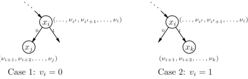
Let us assume that _xi is the selector variable of_νi (in this case,_i ≤ _i by construction). There are two cases:

1 1 0 0 xi xi xj (. . . , νi, νi+1, . . . , νi) (. . . , νi, νi+1, . . . , νi) (νi+1, νi+2, . . . , νj) ... ... Case 1: vi= 0 xk (νi+1, νi+2, . . . , νk) Case 2: vi= 1

Fig. 4.Severalν’s refer to the same BDD node.νjandν_kare the last in the sequence.

– _vi = 0. Let us take_jsuch that_νj is the false child of_νi and the selector vari-able of_νj is_xj (see Figure 4). Then,_γi ≤_γjby definition of the algorithm.

Using the induction hypothesis:

γi ≤_{γj< aj}+1vj+1+· · ·+anvn ≤ai+1vi+1+· · ·+anvn.

– _vi = 1. Similarly, let us take _ksuch that_νk is the true child of_νi and the

selector variable of_νk is_xk (see Figure 4). Then,_γi ≤γ_k+a_iby definition

of the algorithm. Using the induction hypothesis and that_vi= 1:

γi ≤_ai+_{γk < ai}+_ak+1vk+1+· · ·+anvn≤ai+1vi+1+· · ·+anvn.

Therefore, it holds that_{γi< ai}+1v_i+1+· · ·+a_nv_n for everyi. In particular, it

holds for_i= 1. Since the assignment satisfies the PB constraint by hypothesis, we have

γ1< a1v1+· · ·+anvn≤K,

and hence_K does not belong to the theoretical interval of the root node. Notice that if Bis not the BDD of_C some of the computed intervals might be empty. However, the algorithm will be able to compute the remaining intervals and, since the interval of the root node will be empty, the algorithm will also be correct. We are now ready for the following result.

Theorem 6. Unless NP=co-NP, there are PB constraints that do not admit polynomial BDDs.

Proof. A well-known NP-complete problem is the following (variant of the) sub-set sum problem: given a set of integers{a1, . . . , an} and an integer K, decide

whether there exists a subset of {a1, . . . , an} that sums to exactlyK. Here we

prove that if a polynomial-size BDD existed for every PB constraint then for ev-ery unsatisfiable subset sum problem a polynomial-size unsatisfiability certificate would exist, that could moreover be verified in polynomial time, thus collaps-ing NP and co-NP. Indeed, obviously, a subset sum problem ({a1, . . . , a_n}, K)

is unsatisfiable if, and only if, the PB constraints_a1x1+· · ·+a_nx_n ≤K and

a1x1+· · ·+a_nx_n ≤ K −1 are equivalent, i.e., they are the same Boolean

function. So if the subset sum problem ({a1, . . . , an}, K) is unsatisfiable, and a

polynomial-size BDD for_a1x1+· · ·+anxn ≤K existed, this BDD would also

represent_a1x1+· · ·+anxn ≤K−1, which, as we proved in the previous

theo-rem, can be checked in polynomial time (for both PB constraints at once). We find it quite surprising that, even for the limited kind of monotonic functions that can be represented by a single PB constraint, the existence of polynomial-size BDDs would imply NP=co-NP. As said, to our knowledge it remains unknown whether there exists a family of PB constraints that admit no polynomial-size BDD. This situation is analogous to what happens with extended resolution in Cook’s program for propositional proof complexity: it is unknown whether there exists a family of propositional problems that admit no polynomial-size extended resolu-tion proof. So, finding successively more compact unsatisfiability certificates for subset sum might be an interesting alternative to Cook’s program for attacking the NP vs co-NP question.

4

Avoiding Exponential BDDs

In this section we introduce our positive results. We restrict ourselves to a par-ticular class of PB constraints, where all coefficients are powers of two. As we will show below, these constraints admit polynomial BDDs. Moreover, any PB constraint can be reduced to this class.

Example 6. Let us take the PB constraint 9_x1+ 8x2+ 3x3 ≤10. Considering

the binary representation of the coefficients, this constraint can be rewritten into (23_x3,1+ 20x0,1) + (23x3,2) + (21x1,3+ 20x0,3)≤10 if we add the binary clauses

expressing that_xi,r=_xr for appropriate_iand_r.

4.1 Power-of-Two PB Constraints Do Have Polynomial-Size BDDs Let us consider a PB constraints of the form:

C: 20·_δ0,1·x0,1 + 20·δ0,2·x0,2 +· · · + 20·δ0,n·x0,n +

21·_δ1,1·x1,1 + 21·δ1,2·x1,2 +· · · + 21·δ1,n·x1,n +

. . . +

2m·_δm,1·xm,1+ 2m·δm,2·xm,2+· · · + 2m·δm,n·xm,n≤K,

where_δi,r ∈ {0_,1} for all_i and_r. Notice that every PB constraint whose coef-ficients are powers of 2 can be expressed in this way. Let us consider its BDD representation with the ordering_x0,1< x0,2< . . . < x0,n< x1,1< . . . < xm,n.

Lemma 7. Let [_{β, γ}] be the interval of a node with selector variable_xi,r. Then

2i divides_β and0≤_{β <}(_n+_r−1)·2i.

Proof. By Proposition 2.1,_βcan be expressed as a sum of coefficients all of which are multiples of 2i, and hence _β itself is a multiple of 2i. By Proposition 2.7, the only node whose interval contains negative values is the False node, and hence_β 0. Now, using Proposition 2.3, there must be an assignment to the variables{x0,1, . . . , xi,r−1} such that 20δ0,1x0,1+· · ·+ 2iδi,r−1xi,r−1 belongs to

the interval. Therefore:

β≤20_δ0,1x0,1+· · ·+ 2iδi,r−1xi,r−1≤20+ 20+· · ·+ 2i

=_n20+_n21+· · ·+_n2i−1+ (_r−1)·2i=_n(2i−1) + 2i(_r−1)

<2i(_n+_r−1)

Corollary 8. The number of nodes with selector variable _xi,r is bounded by

n+_r−1. In particular, the size of the BDD belongs toO(_n2

m).

Proof. Let_ν1, ν2, . . . , νt be all the nodes with selector variablexi,r. Let [βj, γj]

the interval of _νj. Note that such intervals are pair-wise disjoint since a non-empty intersection would imply that there exists a constraint represented by two different BDDs. Hence we can assume, w.l.o.g., that_β1 < β2 < · · · < β_t.

Due to Lemma 7, we know that _βj−_βj−1 2i. Hence 2i(n+r−1) > β_t

4.2 A Consistent Encoding for PB Constraints

Let us now take an arbitrary PB constraint_C:_a1x1+· · ·anxn ≤Kand assume

that _aM is the largest coefficient. For _m= log_aM, we can rewrite _C splitting the coefficients into powers of two as shown in Example 6:

˜ C: 20_· δ0,1·x0,1 + 20·δ0,2·x0,2 +· · · + 20·δ0,n·x0,n + 21_· δ1,1·x1,1 + 21·δ1,2·x1,2 +· · · + 21·δ1,n·x1,n + . . . + 2m·_δm,1·x_m,1+ 2m·δ_m,2·x_m,2+· · · + 2m·δ_m,n·x_m,n≤K,

where_δm,rδm−1_,r · · · δ0_,r is the binary representation ofa_r. Notice thatCand

˜

C represent the same constraint if we add clauses expressing that _xi,r =_xi for appropriate_i and _r. This process is calledcoefficient decomposition of the PB constraint. A similar idea can be found in [BBR03].

The important remark is that, using a consistent SAT encoding of the BDD for ˜_C (e.g. the one given in [ES06] or the one presented in the next section) and adding clauses expressing that _xi,r = _xi for appropriate _i and _r, we obtain a consistent encoding for the original constraint _C using O(_n2_log

aM) auxiliary variables and clauses.

This is not difficult to see. Take an assignment _A over the variables of _C which cannot be extended to a model of _C. This is because the coefficients corresponding to the variables true in_Aadd more than_K. Using the clauses for

xi,r =_xi, unit propagation will produce an assignment to the_xi,r’s that cannot be extended to a model of ˜_C. Since the encoding for ˜_Cis consistent, a false clause will be found. Conversely, if we consider an assignment_Aover the variables of_C than can be extended to a model of_C, this assignment can clearly be extended to a model for ˜_C and the clauses expressing_xi,r =_xi. Hence, unit propagation on those clauses and the encoding of ˜_C will not detect a false clause.

4.3 An Arc-Consistent Encoding for PB Constraints

Unfortunately, the previous approach does not produce an arc-consistency en-coding. The intuitive idea can be seen in the following example:

Example 7. Let us consider the constraint 3_x1+ 4x2 ≤ 6. After splitting the

coefficients into powers of two, we obtain_C:_x0_,1+ 2x1_,1+ 4x2_,2≤6. If we set

x2_,2to true,C implies that eitherx0_,1orx1_,1have to be false, but the encoding

cannot exploit the fact that both variables will receive the same truth value and hence both should be propagated. Adding clauses stating that_x0,1=x1,1 does

not help in this sense.

In order to overcome this limitation, we follow the method presented in [BKNW09, BBR09]. Let _C : _a1x1+· · ·+anxn ≤ K be an arbitrary PB

con-straint. We denote as_Ci the constraint_a1x1+· · ·+ai·1 +· · ·+anxn≤K, i.e.,

the constraint assuming_xi to be true. For every_iwith 1≤_i≤_n, we encode_Ci as in Section 4.2 and, in addition, we add the binary clause_ri∨ ¬x_i, where _ri

is the root of the BDD for_Ci. This clause helps us to preserve arc-consistency: given an assignment_Asuch that_A∪ {x_i} cannot be extended to a model of_C, literal_riwill be propagated using_A(because the encoding for_Ciis consistent). Hence the added clause will allow us to propagate_xi.

All in all, the suggested encoding is arc-consistent and uses O(_n3log(_aM)) clauses and auxiliary variables, where_aM is the largest coefficient.

5

SAT Encodings of BDDs for Monotonic Functions

In this section we consider a BDD representing a monotonic function_F and we want to encode it into SAT. As expected, we want the encoding to be as small as possible and arc-consistent.

As usual, the encoding introduces an auxiliary variable for every node. Let_ν be a node with selector variable_xand auxiliary variable_n. Let_f be the variable of its false child and_tbe the auxiliary variable of its true child. Only two clauses per node are needed:

¬f → ¬n ¬t∧x→ ¬n.

Furthermore, we add a unit clause with the variable of the True node and another one with the negation of the variable of the False node.

Theorem 9. The encoding is consistent in the following sense: a partial assign-ment_A cannot be extended to a model of _F if and only if ¬r is propagated by unit propagation, where _ris the root of the BDD.

Proof. We prove the theorem by induction on the number of variables of the BDD. If the BDD has no variables, then the BDD is either the True node or the False node and the result is trivial.

Assume that the result is true for BDDs with less than_kvariables, and let_F be a function whose BDD has_kvariables. Let_rbe the root node,_x1its selector

variable and_{f, t}respectively its false and true children (note that we abuse the notation and identify nodes with their auxiliary variable). We denote by_F1 the

function_F|x1=1 (i.e.,F after settingx1to true) and byF0 the functionF_|x1=0.

– Let_Abe a partial assignment that cannot be extended to a model of_F.

• Assume_x1 ∈A. Since Acannot be extended, the assignment A\ {x1}

cannot be extended to a model of _F1. By definition of the BDD, the

function_F1 hast as a BDD. By induction hypothesis,¬tis propagated,

and since_x1∈A,¬ris also propagated.

• Assume_x1∈A. Then, the assignmentA\ {¬x1}cannot be extended to

a model of_F0. SinceF0 hasf as a BDD, by induction hypothesis¬f is

propagated, and hence¬ralso is.

– Let_A be a partial assignment, and assume¬rhas been propagated. Then, either ¬f has also been propagated or¬t has been propagated and_x1 ∈A

(note that_x1has not been propagated because it only appears in one clause

• Assume that ¬f has been propagated. Since _f is the BDD of _F0, by

induction hypothesis the assignment_A\ {x1,¬x1} cannot be extended

to a model of_F0. Since the function is monotonic,A\ {x1,¬x1}neither

can be extended to a model of_F. Therefore,_Acannot be extended to a model of_F.

• Assume that¬thas been propagated and_x1∈A. Sincetis the BDD of

F1, by induction hypothesisA\ {x1} cannot be extended to a model of

F1, so neither canA be extended to a model ofF.

For obtaining an arc-consistent encoding, we only have to add a unit clause. Theorem 10. If we add a unit clause forcing the variable of the root node to be true, the previous encoding becomes arc-consistent.

Proof. We will prove it by induction on the variables of the BDD. The case_n= 0 is trivial, so let us prove the induction case.

As before, let_rbe the root node,_x1its selector variable andf, tits false and

true children. We denote by_F1 andF1 the functionsF|x₁=1and F|x₁=0.

Let_Abe a partial assignment that can be extended to a model of_F. Assume that_A∪ {x_i}cannot be extended. We want to prove that_xi will be propagated. – Let us assume that _x1 ∈A. In this case, t is propagated due to the clause

¬t∧x1 → ¬nand the unit clausen. Since x1∈Aand A∪ {xi} cannot be

extended to a model of _F, _A\ {x1} ∪ {xi} neither can be extended to an

assignment satisfying_F1. By induction hypothesis, sincetis the BDD of the

function_F1,¬xi is propagated.

– Let us assume that _x1 ∈ A and x_i = x1. Since F is monotonic, A∪ {x_i}

cannot be extended to a model of_F if and only if it cannot be extended to a model of_F0. Notice thatf is propagated thanks to the clause ¬f →nand

the unit clause_n. By induction hypothesis, the method is arc-consistent for

F0, soxiis propagated.

– Finally, assume that_x1∈Aandxi =x1. SinceA∪{x1}cannot be extended

to a model of_F, _Acannot be extended to model of _F1. By Theorem 9,¬t

is propagated and, due to¬t∧_x1→ ¬nandn, also is¬x1.

6

Conclusions and Future Work

Both theoretical and practical contributions have been made. Regarding the the-oretical part, we have proved that, unless NP=co-NP, there are PB constraints that do not admit polynomial BDDs. The existence of a concrete PB constraint family for which no polynomial BDDs exist remains an open problem, with inter-esting connections to the area of proof complexity. One of our aims is to continue working on this open question in the near future.

At the practical level, we have introduced a BDD-based polynomial and consistent encoding of PB constraints and we have developed a BDD-based arc-consistent encoding of monotonic functions that only uses two clauses per BDD node. Indeed our initial motivation for this work has been practical, and we are currently working on implementation and experimental comparison of our encodings with other existing approaches on realistic problems.

References

[BBR06] Bailleux, O., Boufkhad, Y., Roussel, O.: A Translation of Pseudo Boolean Constraints to SAT. JSAT 2(1-4), 191–200 (2006)

[BBR09] Bailleux, O., Boufkhad, Y., Roussel, O.: New Encodings of Pseudo-Boolean Constraints into CNF. In: Kullmann, O. (ed.) SAT 2009. LNCS, vol. 5584, pp. 181–194. Springer, Heidelberg (2009)

[BBR03] Bartzis, C., Bultan, T.: Construction of efficient BDDs for Bounded Arithmetic Constraints. In: Garavel, H., Hatcliff, J. (eds.) TACAS 2003. LNCS, vol. 2619, pp. 394–408. Springer, Heidelberg (2003)

[BHvMW09] Biere, A., Heule, M.J.H., van Maaren, H., Walsh, T. (eds.): Handbook of Satisfiability. IOS Press, Amsterdam (2009)

[BKNW09] Bessiere, C., Katsirelos, G., Narodytska, N., Walsh, T.: Circuit Com-plexity and Decompositions of Global Constraints. In: IJCAI 2009, pp. 412–418 (2009)

[Bry86] Bryant, R.E.: Graph-based algorithms for boolean function manipula-tion. IEEE Trans. Computers 35(8), 677–691 (1986)

[ES06] E´en, N., S¨orensson, N.: Translating Pseudo-Boolean Constraints into SAT. JSAT 2, 1–26 (2006)

[J.S07] Smaus, J.: On Boolean Functions Encodable as a Single Linear Pseudo-Boolean Constraint. In: Van Hentenryck, P., Wolsey, L.A. (eds.) CPAIOR 2007. LNCS, vol. 4510, pp. 288–302. Springer, Heidelberg (2007)

[SFSW09] Schutt, A., Feydy, T., Stuckey, P.J., Wallace, M.: Why Cumulative De-composition Is Not as Bad as It Sounds. In: Gent, I.P. (ed.) CP 2009. LNCS, vol. 5732, pp. 746–761. Springer, Heidelberg (2009)