Decision making with the analytic network process

(1)

DECISION MAKING WITH THE ANALYTIC NETWORK PROCESS

Nikola Kadoić

Faculty of Organisation and Informatics Pavlinska 2, Varaždin, Croatia

Nina Begičević Ređep

Blaženka Divjak

Abstract: One of the most advanced and complex multi-criteria decision-making methods is the analytic network process (ANP). This method supports modelling dependencies and feedback between elements in the network. For this reason, the ANP is one of the most appropriate methods for making decisions in fields that are characterised by existing dependencies of higher-level elements on lower level elements. In addition to reviewing the ANP, this paper also studies some possible method upgrades that might decrease the complexity of the original ANP. We explore this by structuring the problem as a weighted graph and using the concept of compatibility between interdependent matrices in the ANP. Keywords: analytic network process, dependencies, influences, feedback, structuring, weighted

graph, interdependent matrices 1 INTRODUCTION

When we talk about multi-criteria decision making, many methods can be used. The most well-known multi-criteria decision-making method is the analytic hierarchy process (AHP). In that method, the decision-making problem is decomposed into a hierarchy. At the top of the hierarchy is the decision-making goal. The criteria are on the next level, which can be decomposed to the sub-criteria (and further decomposed to the lower levels). On the last level are the alternatives. By using pairwise comparisons (to be explained later in this paper), local priorities of alternatives as well as criteria weights are calculated. Then, it is possible to calculate global priorities of alternatives and make decisions.

In the decision-making problem field, if influences/dependencies exist between criteria, which the AHP does not consider, using the AHP might lead to a decision that is less than optimal. In those cases, using the analytic network process (ANP) is more appropriate. By using the ANP, we can model the dependencies and feedback between the decision-making elements, and calculate more precise weights of criteria, and local and global priorities of alternatives. In this paper, we will describe the ANP method, present its steps using a demonstrative example (Section 2), address some weaknesses of the method based on a literature review and our experience, and propose some upgrades to the ANP that might impact on eliminating the identified weaknesses (Section 3).

2. THE ANALYTIC NETWORK PROCESS (ANP)

The decision-making problems in the ANP are modelled as networks, not as hierarchies as with the AHP. The ANP is a generalisation of the AHP. Figure 1 presents the structural differences

(2)

between a linear hierarchy and a nonlinear network. The basic elements in the hierarchy and network are clusters (components; rectangles and ellipses in Figure 1), nodes (elements in clusters, not specified in Figure 1) and dependencies (arcs). The meaning of ‘depend on’ is the opposite of ‘have an influence on’.

Figure 1: Structural difference between hierarchy and network (adapted from [1])

The left side of Figure 1 shows a linear network (hierarchy) in which elements from the lower level of the network have an influence on a higher level, e.g. criteria have an influence on the goal, which means that the goal depends on the criteria. On the right side of Figure 1, we have a network of clusters and some possible dependencies between them. In this case, it is possible for a cluster to depend on another cluster, but at the same time, it can influence the same one or even itself.

The steps of the ANP [2], [3] will be described through a simple example, evaluation of scientists.

Figure 2: Structure of decision-making problem, ‘evaluation of scientists’

Problem structuring. The goal of the decision making is to select the best scientists among three scientists. This means that we will have: (1) cluster Goal with node G; (2) clusters

Alternatives with three nodes, alternatives A1, A2 and A3; and (3) five nodes of criteria (papers

Goal Criteria Sub-criteria Alternatives Source Component Intermediate Component Source Component Intermediate Component Intermediate Component C 1 C₂ C 5 C 4 C 4 pa pr ci co gr G A1 A2 A3 Cluster ‘Goal’ Cluster ‘Science’ Cluster ‘Teaching’ Cluster ‘Alternatives’ Goal Science _Teaching Alternatives

(3)

– pa, citations – ci, projects – pr, courseware – co, grades from students – gr) grouped into two clusters (Science – first three criteria and Teaching – last two criteria).

The problem structure is shown in Figure 2 (left). Solid arcs (arrows) are related to the dependencies of the goal on criteria. Dashed arcs are related to the dependencies between criteria. Dotted arcs are related to the dependencies of alternatives on criteria and dependencies of criteria on alternatives. Arcs between alternatives and criteria, pa and co, are not shown because of the complexity of the figure, but those dependencies also exist. The decision-making structure can be shown in a simpler way (with information lost), Figure 2 (right). The

Goal is a source cluster that depends on Science and Teaching (black arcs). The other three clusters are intermediate components. The dashed arc between Science and Teaching is the result of the existence of at least one arc between at least one criteria from Science and at least one criteria in Teaching, e.g. pr depends on co. The dashed arc between Teaching and Science

can be interpreted similarly. The loops in the clusters, Science and Teaching, are the result of the existence of at least one dependency of one criterion to another in the same cluster, e.g. ci

depends on pa, or gr depends on co.

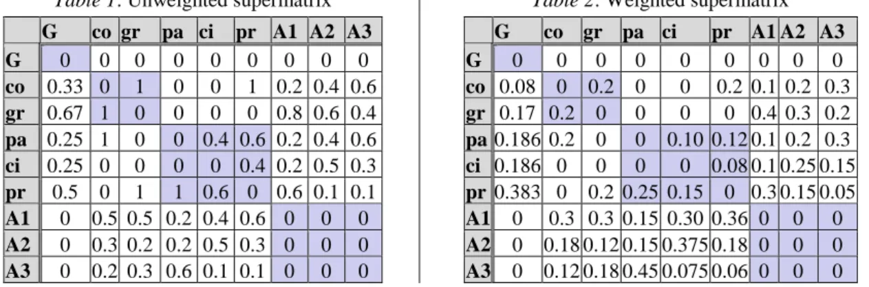
Pairwise comparisons on node level. Now, we should create the unweighted supermatrix. It is a square matrix of all nodes in the decision-making problem and contains local priorities. When making judgements in pairwise comparisons, we use Saaty’s fundamental scale of absolute numbers [4], just as with the AHP. The scale has nine different intensities: 1 means that two elements in a pair are equally important with respect to the higher level element; 9 means extreme importance of one element over another. All real numbers between 1 and 9 can be used. Because of the axiom of reciprocity, we use reciprocal numbers of 1–9 as well [5]. When making the pairwise comparisons, we must take care of inconsistencies. If we say that element A is greater than element B, and B is greater than C, then, because of transitivity, A is greater than C. There is an inconsistency ratio, a measure that describes how inconsistent the decision maker was during the pairwise comparisons procedure. The allowed inconsistency ratios are all under 10%. See more in [3].

To fill the unweighted supermatrix (Table 1) with priorities, we have to make pairwise comparisons of nodes with respect to other nodes. The comparisons that have to be done are:

- Comparisons of the criteria with respect to the goal (see black arcs in Figure 2): comparisons of criteria in Science with respect to G (local priorities will be put into the supermatrix at rows ci, pr, pa and column G); comparisons of criteria in Teaching

with respect to G (local priorities will be put into the supermatrix at rows co, gr and column G);

Calculations to get priorities for co and gr are as follows:

G co gr AVG

co 1 0.5 0.33 0.33 0.33 gr 2 1 0.67 0.67 0.67

3 1.5

Create a matrix of comparisons (coloured in grey). Put 1 on the diagonal (co is equally important as co). Make pairwise comparisons to fill the other cells. We ask the question, ‘With respect to the goal, which criterion is more important, co or gr?’ Let us say that the answer is that gr is more important than co, 2 on Saaty’s scale. We put

2 on position (gr, co) and the reciprocal number (0.5) on position (co, gr) in a matrix of comparisons. Then, we sum the columns. We make the new matrix in which each value from the comparison matrix will be divided by the related column sum. Then,

(4)

we calculate the average of the rows of that second matrix. We fill the supermatrix with (co, G) = 0.33 and (gr, G) = 0.67;

- Comparisons of criteria with respect to other criteria – comparisons of the criteria that leave (influence) the same criterion from the same cluster with respect to it (see dashed arcs in Figure 2): pa and pr with respect to ci; pa and ci with respect to pr; pa and pr

with respect to co. Priorities are put into the supermatrix depending on which criteria (rows) influence which criterion (column). When making a pairwise comparison between pa and pr with respect to ci, we try to answer the question, ‘Which criterion,

pa or pr, has a higher influence on criterion ci, and by how much?’ When some criteria depend on only one criterion in the same cluster, we do not make a comparison, and write 1 in the related cell in the supermatrix, e.g. cell (pr, pa) = 1;

- Comparisons of alternatives with respect to each criterion (see dotted arcs from criteria to alternatives in Figure 2), the same as in the AHP. This will fill part of the supermatrix as follows: rows A1, A2 and A3, columns co, gr, pa, ci, pr;

- Comparisons of criteria in each cluster with respect to each alternative (see the dotted arc from alternatives to criteria in Figure 2). This will fill part of the supermatrix as follows: rows co, gr, pa, ci, pr, columns A1, A2 and A3. For example, let us say that alternative A1 has a good value in terms of criterion co, and a very bad value in terms of gr. Let us use 4 on Saaty’s scale to describe this importance; then, at column A1, in rows co and gr, we will write 0.2 and 0.8, respectively.

Pairwise comparisons on a cluster level. The goal of this step is to convert the unweighted matrix into the weighted supermatrix. For this, we have to do the following comparisons:

- Compare two clusters of criteria with respect to the Goal. For example, if we say that cluster Science is more important than Teaching, 3 in Saaty’s scale, by using the same

pairwise comparisons procedure as when comparing the nodes, we will get weights 0.25 (Teaching) and 0.75 (Science). This means that 0.25 will multiply Teaching’s

criteria and 0.75 will multiply Science’s criteria in column G;

- Compare clusters Teaching, Science and Alternatives with respect to Teaching; - Compare clusters Teaching, Science and Alternatives with respect to Science; and - Compare clusters Teaching and Science with respect to Alternatives.

Table 1: Unweighted supermatrix Table 2: Weighted supermatrix

G co gr pa ci pr A1 A2 A3 G 0 0 0 0 0 0 0 0 0 co 0.33 0 1 0 0 1 0.2 0.4 0.6 gr 0.67 1 0 0 0 0 0.8 0.6 0.4 pa 0.25 1 0 0 0.4 0.6 0.2 0.4 0.6 ci 0.25 0 0 0 0 0.4 0.2 0.5 0.3 pr 0.5 0 1 1 0.6 0 0.6 0.1 0.1 A1 0 0.5 0.5 0.2 0.4 0.6 0 0 0 A2 0 0.3 0.2 0.2 0.5 0.3 0 0 0 A3 0 0.2 0.3 0.6 0.1 0.1 0 0 0 G co gr pa ci pr A1 A2 A3 G 0 0 0 0 0 0 0 0 0 co 0.08 0 0.2 0 0 0.2 0.1 0.2 0.3 gr 0.17 0.2 0 0 0 0 0.4 0.3 0.2 pa 0.186 0.2 0 0 0.10 0.12 0.1 0.2 0.3 ci 0.186 0 0 0 0 0.08 0.1 0.25 0.15 pr 0.383 0 0.2 0.25 0.15 0 0.3 0.15 0.05 A1 0 0.3 0.3 0.15 0.30 0.36 0 0 0 A2 0 0.18 0.12 0.15 0.375 0.18 0 0 0 A3 0 0.12 0.18 0.45 0.075 0.06 0 0 0

Calculating the limit matrix. In this step, the weighted matrix is multiplied by itself as long as all of its columns become equal. This is how we get the final priorities. After this step, the sensitivity analysis is performed. Software called Superdecisions supports all the math behind the ANP (webpage: https://www.superdecisions.com/, Creative Decisions Foundation). Therefore, we did not go into detail about what this particular software supports.

(5)

3 PROPOSALS OF THE ANP UPGRADES

We focussed on the steps that users have repeatedly used, because according to our own experiences, many still do not completely understand the ANP. For example, the field of higher education is characterised by existing dependencies between criteria and feedback in decision-making problems. However, the literature review about which decision-decision-making methods have been used in practice to solve problems showed that the AHP method was used most, and the ANP was rarely used [6]. The weaknesses of the ANP are related to the complexity of the method, the duration of implementation, and uncertainty in giving judgements, especially those on the cluster level [7]. When looking at the supermatrix, we conclude that the column of the goal and the rows of the alternatives are related to the AHP. This part is understood by the users. Some problems can appear in situations with a large number of alternatives, which can increase the duration of decision making. One solution to this is ratings as explained in [1], [4].

Our focus, in terms of proposing upgrades to decrease some ANP weaknesses, is related to calculating other parts of the supermatrix, not those that are related to the AHP. There are two parts of the supermatrix that can be calculated differently:

- The first part is related to the priorities of criteria with respect to criteria (because of dependencies between the criteria in the network); and

- The second part is related to the priorities of criteria with respect to alternatives (because of dependencies of alternatives on criteria).

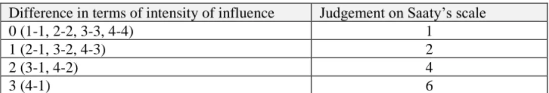
The first upgrade requires a slightly different problem structuring procedure than the regular ANP. In the ANP, we model dependencies between criteria. Then, to make comparisons between criteria with respect to the criteria, we have to know the intensity of influences (dependencies) between criteria. We propose structuring the problem by using a weighted graph. So, to start, when we model dependencies between criteria, we also define the intensities of dependencies. Indeed, during the problem-structuring procedure, to draw an arc between two criteria, the decision maker should think deeply about the relationship between two criteria. During that process, (s)he is evaluating the influence of the dependency between two criteria. A similar problem-structuring procedure can be found in the decision-making trial and evolution laboratory (DEMATEL) method. In DEMATEL, instead of the dependencies, arcs represent influences between criteria. Thus, it is possible to structure the problem by using the approach from the DEMATEL and transform it from graphs with influences onto the graph of dependencies, keeping the intensities of dependencies the same. In DEMATEL, the intensities of the influences between criteria are measured on a scale of 5 degrees: 0 means no influence, and 4 means very high influence [8].

Now, when we have a weighted graph of dependencies between criteria, we can automatize the calculation of the limit matrix. One method of automatization is to apply the normalisation by sum and another method is to use a matrix of transition. A proposed matrix of transition is given in Table 3.

Table 3: Matrix of transition

Difference in terms of intensity of influence Judgement on Saaty’s scale

0 (1-1, 2-2, 3-3, 4-4) 1

1 (2-1, 3-2, 4-3) 2

2 (3-1, 4-2) 4

3 (4-1) 6

For example, on one hand, to calculate the local priorities of pa and pr in column ci with identified intensities of influences 2 and 3 for pa->ci and pr->ci, respectively, we apply the

(6)

normalisation by sum and get priorities 0.4 and 0.6. On the other hand, if we use a matrix of transition for the difference 1 in terms of intensity of influence, we get priorities 0.33 and 0.67. We tested this approach on several examples, and at times, one method showed closer results to the ANP results, and sometimes, the other. An average of both methods can also be an approach.

In this ANP upgrade, local priorities in terms of dependencies between criteria are calculated automatically. The main advantage of this approach is that the total implementation process takes less time than the regular ANP. Also, users do not have to make judgements and risk making wrong judgements because of their misunderstanding of pairwise comparisons of two criteria with respect to a third.

The second upgrade is related to applying the concept of compatibility between interdependent matrices in the ANP. By using this approach, the process of calculating the priorities of criteria with respect to alternatives can be shortened. An analysis of the compatibility between interdependent matrices in the ANP is explained in the paper [9].

For example, the original data about values of alternatives A1, A2 and A3 in terms of criteria

pa, ci, pr are given in Table 4.

Table 4: Evaluation of scientists Alternatives pa ci pr A1 5 40 6 A2 5 50 3 A3 15 10 4

When calculating the priorities of the alternatives with respect to criteria (as with the AHP), we made comparison tables as illustrated in Table 5. When we make comparisons of criteria per alternatives, we are taking into account the same data from Table 4 when we make comparisons of the alternatives with respect to the criteria. The concept of compatibility between interdependent matrices in the ANP can now be applied.

Table 5: Comparisons of alternatives with respect to criteria

pa A1 A2 A3 ci A1 A2 _A3 pr A1 A2 A3 A1 1 1 0.25 _A1 1 0.5 3 _A1 1 5 4 A2 1 1 0.25 _A2 2 1 4 _A2 0.2 1 0.5 A3 4 4 1 _{A3 0.33 0.25} 1 _{A3 0.25} 2 1 When we make comparisons of criteria with respect to, for example, A1, we can make any matrix of comparisons of criteria that is consistent at the local level, but inconsistent at the global level. An example is given in Table 6. The inconsistency ratio of the matrix is 0.00, but the comparisons are illogical. In Table 4, we see that A1 has a low value in terms of criteria pa, and a high value in terms of criterion pr. That means that pr dominates over pa; however, in Table 6, we make the opposite judgement with an acceptable inconsistency ratio.

Table 6: Comparisons of criteria with respect to A1

A1 pa ci pr

pa 1 2 4

ci 0.5 1 2

(7)

However, to use the concept of compatibility between interdependent matrices in the ANP, we need to do one comparison matrix, and others can be calculated automatically. An example is given in Table 7. Comparisons with respect to A1 have to be manually input, while comparisons with respect to A2 and A3 are automatically calculated.

Let us say that pr dominates over pa with respect to A1 – with 5 on Saaty’s scale (according to the values in Table 4). Because A1 and A2 are equally important with respect to pa, and A1 dominates over A2 with respect to pr with 5 (see Table 5), pr becomes equally important as pa

with respect to A2. Similarly, we calculate other values.

Table 7: Comparisons of criteria with respect to alternatives

A1 pa ci pr A2 pa ci pr A3 pa ci pr

pa 1 0.33 0.2 _pa 1 0.17 1 _pa 1 0.25 3.2

ci 3 1 0.5 ci 6 1 5 ci 4 1 0.5

pr 5 2 1 _pr 1 0.2 1 _pr 0.31 2 1 4 CONCLUSION

In this paper, we gave an overview of the ANP method with a detailed illustration of the steps that we find crucial in the ANP, and which are often still not understood by users. Conducting the ANP is a time-consuming activity, and some steps are very challenging. Therefore, we proposed two upgrades of how to automatize some parts of the ANP to be less complex and more appropriate for users.

Acknowledgement

Croatian Science Foundation has partly supported this paper under the project Higher Decision, IP-2014-09-7854.

References

[1] T. L. Saaty and L. G. Vargas, Decision Making with the Analytic Network Process: Economic,

Political, Social and Technological Applications with Benefits, Opportunities, Costs and Risks.

Springer; Softcover reprint of hardcover 1st ed. 2006 edition (December 28, 2009), 2006. [2] T. L. Saaty and B. Cillo, A Dictionary of Complex Decision Using the Analytic Network Process,

The Encyclicon, Volume 2, 2nd ed. Pittsburgh: RWS Publications, 2008.

[3] N. Begičević, “Višekriterijski modeli odlučivanja u strateškom plniranju uvođenja e-učenja,” University of Zagreb, Faculty of organization and informatics, 2008.

[4] T. L. Saaty, “Decision making with the analytic hierarchy process,” Int. J. Services Sciences, vol. 1, no. 1, pp. 83–98, 2008.

[5] P. T. Harker and L. G. Vargas, “The Theory of Ratio Scale Estimation: Saaty’s Analytic Hierarchy Process,” Management Science, vol. 33, no. 11, pp. 1383–1403, Nov. 1987.

[6] N. Kadoić, N. Begičević Ređep, and B. Divjak, “E-learning decision making: methods and methodologies,” in Re-Imagining Learning Scenarios, 2016, vol. CONFERENCE, no. June, p. 24.

[7] N. Kadoić, B. Divjak, and N. Begičević Ređep, “Effective Strategic Decision Making on Open and Distance Education Issues,” in Diversity Matters!, 2017, pp. 224–234.

[8] J. Shao, M. Taisch, M. Ortega, and D. Elisa, “Application of the DEMATEL Method to Identify Relations among Barriers between Green Products and Consumers,” 17th European Roundtable

on Sustainable Consumption and Production - ERSCP 2014, pp. 1029–1040, 2014.

[9] L. C. Leung, Y. V Hui, and M. Zheng, “Analysis of compatibility between interdependent matrices in ANP,” Journal of the Operational Research Society, vol. 54, no. 7, pp. 758–768, Jul. 2003.