for driving applications
Iv´an del Pino?, V´ıctor Vaquero?, Beatrice Masini, Joan Sol`a, Francesc Moreno-Noguer, Alberto Sanfeliu, and Juan Andrade-Cetto Institut de Rob`otica i Inform`atica Industrial, CSIC-UPC
Llorens Artigas 4-6, 08028 Barcelona, Spain.
{idelpino,vvaquero,bmasini,jsola,fmoreno,sanfeliu,cetto}@iri.upc.edu http://www.iri.upc.edu
Abstract. Vehicle detection and tracking in real scenarios are key com-ponents to develop assisted and autonomous driving systems. Lidar sen-sors are specially suitable for this task, as they bring robustness to harsh weather conditions while providing accurate spatial information. How-ever, the resolution provided by point cloud data is very scarce in com-parison to camera images. In this work we explore the possibilities of Deep Learning (DL) methodologies applied to low resolution 3D lidar sensors such as the Velodyne VLP-16 (PUCK), in the context of vehicle detection and tracking. For this purpose we developed a lidar-based sys-tem that uses a Convolutional Neural Network (CNN), to perform point-wise vehicle detection using PUCK data, and Multi-Hypothesis Extended Kalman Filters (MH-EKF), to estimate the actual position and veloci-ties of the detected vehicles. Comparative studies between the proposed lower resolution (VLP-16) tracking system and a high-end system, using Velodyne HDL-64, were carried out on the Kitti Tracking Benchmark dataset. Moreover, to analyze the influence of the CNN-based vehicle detection approach, comparisons were also performed with respect to the geometric-only detector. The results demonstrate that the proposed low resolution Deep Learning architecture is able to successfully accom-plish the vehicle detection task, outperforming the geometric baseline approach. Moreover, it has been observed that our system achieves a similar tracking performance to the high-end HDL-64 sensor at close range. On the other hand, at long range, detection is limited to half the distance of the higher-end sensor.
Keywords: Vehicle detection Point cloud Deconvolutional networks Multi-object tracking MHEKF DATMO HDL-64 VLP-16
?
These authors contributed equally. This work has been supported by the Span-ish Ministry of Economy and Competitiveness projects ROBINSTRUCT (TIN2014-58178-R) and COLROBTRANSP (DPI2016-78957-R), by the Spanish Ministry of Education FPU grant (FPU15/04446), the Spanish State Research Agency through the Mar´ıa de Maeztu Seal of Excellence to IRI (MDM-2016-0656) and by the EU H2020 project LOGIMATIC (H2020-Galileo-2015-1-687534). The authors also thank Nvidia for hardware donation under the GPU grant program.
1
Introduction
The ability to identify and to consistently track vehicles over time is crucial for the development of Advanced Driving Assistance Systems (ADAS) and Au-tonomous Driving (AD) applications. A robust vehicle tracking module is a powerful base block to elaborate further systems, such as traffic merging [31], cruise control [12], lane change [28], collision avoidance [7] or vehicle platooning [1]. Real-world driving scenarios are complex and very dynamic on their own. In addition, the appearance of those scenarios can be greatly affected by a num-ber of factors including context (urban, road, highway, etc), day-time (sunrise, sunset, night, etc) and meteorological conditions (rain, fog, overcast, etc). Opti-cal cameras may fail perceiving correctly the environment in certain conditions, therefore other robust sensors are needed. Lidar technology provides the desired robustness and precision under harsh conditions [21], which make laser scanners suit for autonomous driving applications. Although lidar sensors are expensive compared to artificial vision technologies, recently more affordable models are being introduced into the market. An example is the new Velodyne model VLP-16, which price is an order of magnitude lower than the well known HDL-64 lidar sensor. This fact bridges the gap between technologies, especially taking into account not only the sensor cost, but also the required processing equipment. Lidar point clouds have been traditionally processed following geometrical ap-proaches like in [20]. However, recent works [8], [5] are pointing at Deep Learning techniques as powerful tools to extract information from point clouds, expand-ing their applicability beyond image processexpand-ing tasks. In previous works [26], we developed a vehicle lidar-based tracking system that used a Fully Convolutional Network (FCN) to perform per-point data segmentation using a Velodyne HDL-64 sensor. In this paper we expand the possibilities of this DL segmentation approach, applying it to lower resolution lidar data.We use the Kitti Tracking Benchmark dataset [9], decimating the Velodyne HDL-64 point clouds to match the PUCK sensor descriptions. The resulting low resolution information is used to train a new convolutional architecture for detecting vehicles which outputs are feed into a multi-hypothesis tracker module. The tracking results are fi-nally evaluated using the Kitti evaluation server. We investigate how the sensor
resolution affects the overall system performance through a comparative study using both mentioned sensors. To assess the CNN based vehicle detector module we report the point-wise precision and recall values obtained through a 4-fold cross-validation process. Moreover, we analyze the contribution of the proposed convolutional approach by comparing it with the tracking results obtained using two alternative systems: a geometric detector and an ideal detector that is the pixel level ground truth used to train the network.
2
Related Work
Object Detection in Lidar Point Clouds. Classic approaches for object detection in lidar point clouds use clustering algorithms to segment the data, assigning the resulting groups to different classes [2, 27, 6, 18]. Other strategies, such as the one used as baseline method in this paper, benefit from prior knowl-edge of the environment structure to ease the object segmentation and clustering [20, 24]. 3D voxels can be also created to reduce computational costs by grouping sets of neighbor points. Graphs can be later built on top of grouped voxels to classify them in objects [30, 25, 19]. More recent methods are able to process the point cloud space (raw, or reduced in voxels) to extract hand-crafted features such as spin images, shape models or geometric statistics [3].Vote3D [29] uses this second approach and encodes the sparse lidar point cloud with different features. The resulting representation is scanned in a sliding manner with 3D windows of different sizes, and an SVM followed by a voting scheme is used to classify the final candidate windows.
Deep Learning for Object Detection on Lidar information.Deep learn-ing techniques and Convolutional Neural Networks have been applied with great success to classical computer vision problems such as object classification [13] [11], detection [22], [23], and semantic segmentation [17]. Some early approaches on using CNNs to detect vehicles over 3D lidar point clouds make use of 3D con-volutions [14] or sparse 3D concon-volutions acting as voting weights for predicting the detection scores [8, 10]. However, due to the high dimensionality and sparsity of 3D lidar data, deploying them over point clouds implies high computational burden. Another adopted approach is to apply the well know 2D convolution tools over equivalent 2D representations of the 3D point cloud. In this way, [15] predicts the objectness of each point as well as vehicle 3D bounding boxes by applying a Fully Convolutional Network over a front view representation in which each element encodes a ground-measured distance and height of the corre-sponding 3D point. The recent evolution of [15] combines RGB images with lidar information to generate accurate 3D bounding box proposals, obtaining state of the art results in the detection challenge of the Kitti dataset [5]. However, this method does not fulfill the lidar-only requirement that we impose in our work.
3
System Description
We now describe our full working system for detection and tracking vehicles on lidar data. It is composed of an initial preprocessing step of the lidar informa-tion. Subsequently, a convolutional network performs per-point vehicle detection, which results are later used to obtain bounding boxes of vehicle proposals. Fi-nally, using as additional input the ego-odometry, these vehicle proposals are tracked through time, obtaining information about their poses, dimensions and velocities. The following sections describe the above mentioned modules in detail.
3.1 Data Arrangement
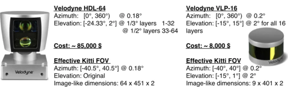
Raw point cloud information is usually received unordered and unsized, as there are missing and multi-reflected beams that produce a variable number of points. In order to ease the geometric processing of information with 2D convolutions we create a more efficient image-like representation by re-arranging each point cloud in a matrix (M) of constant dimensions using spherical coordinates. Each Cartesian point is extracted from the point cloud and transformed to spherical coordinates p(x, y, z, r)→p(φ, θ, ρ, r), whereraims for the energy reflected on each beam. Its angular values are encoded using theM indexes, row for elevation (φ), column for azimuth (θ). In this way, each pair (φ, θ) stores the range (ρ) and reflectivity (r) perceived. As the Kitti tracking benchmark provides only labels for the elements within the front camera field of view, we restrict our 3D point cloud to the corresponding angles. The remaining points are then transformed as specified above. The final dimensions of M depend therefore on the sensor angular resolution (∆φ, ∆θ), which details are specified in Fig. 1. Missing points are labeled with an invalid-point code, and multi-echoes account only for the closer detection. The dataset contains only data of the Velodyne HDL-64 sensor, so we decimate it according to the PUCK specifications. For the VLP-16 sensor, we compose anM matrix of 9×401, whereas in [26] the size was of 64×451 for the HDL-64 lidar. Some examples on theM arrange are shown in Fig. 2. Notice that although specifications in Fig. 1 show 16 vertical layers for the VLP-16 lidar, only 9 geometrically corresponding layers can be extracted from the HDL-64 raw data of the Kitti dataset because the elevation FOV is not coincident between sensors. Nevertheless this is not relevant for the system performance, as the sensor is mounted on the roof of the vehicle and hence the missing layers would point upwards. To get the ground-truth representation needed for the supervised learning process, we use the 3D-oriented bounding boxes expressed in camera frame provided with the Kitti tracklets. Using the available calibration matrices, we convert these bounding boxes to PUCK coordinates and assign an ID to all 3D points lying inside each bounding box. Finally, the generated ground-truth 3D labels are encoded in the image-like space, with pixels assigned to any of the
3.2 Convolutional Network for Lidar Vehicle Detection
Our aim is to classify each 2D pixel encoding a 3D point as belonging to the class
vehicleorbackground, which can be considered as a binary per-pixel classification problem. We therefore seek to find the probability of each pixel to belong to a vehicle or background:p(k|pi), wherek∈ {vehicle, background};i∈1, ...N, and pi∈R3represents each point of the point cloudP of the Euclidean space.
We tackle the stated problem in the same way as in [26], having in mind the recent success of Fully Convolutional Networks architectures [17]. However, as the information provided by the PUCK lidar is scarcer, a simpler architecture composed by two convolution and deconvolution blocks plus the final classifier has been designed. Each block uses 3×15 convolutional filters, followed by a batch normalization and relu non-linearity. In addition max-pooling is used after the convolutional blocks to reduce the output dimensionality.
For the learning process, we back-propagate a Weighted Cross Entropy (WCE) training lossLdefined as,
LW CE=−
H,W,K
X
i,j,k
ω(Yi,j)Id[Yi,j]log( ˆYi,j,k), (1)
whereH, W, K refer to the height, width and channel (class) of the output pre-dictions, ˆY,Y are respectively the predictions and ground-truth classes,Id[x0](x)
is a binary selector function that gets the probability associated to the expected ground truth class. ω(k) is a class-imbalance regularizator computed from the training set statistics as the ratio between background and vehicle points.
3.3 Bounding Box Extraction and Matching
To extract bounding boxes from the set of vehicle points obtained, we apply an Euclidean clustering algorithm. Then, we filtered the obtained groups by size and number of points. The height of the remaining clusters is calculated and stored. Subsequently, we project each cluster into the X −Y plane and keep for each azimuth angle the points with the minimum range, aiming to get the object external perimeter. We fit a 2D oriented bounding box to all the resulting objects, which will give us relevant information to be used by the tracker: width, length, 2D centroid, orientation and fitting error.
The oriented bounding box fitting process consist in performing an angu-lar swept of BB candidates in the [−π
4, π
4) interval. For each candidate we cast simulated 2D PUCK beams following the sensor specification on the azimuth resolution to obtain the geometrically equivalent impact over the boxes. The best 2D fitting box is then chosen as the one with the minimum mean square distance between the real vehicle detected points and the simulated ones. Ob-served bounding boxes are finally compared with the active tracks predicted positions, associating the closest observation-track pair according to a threshold on its Mahalanobis distance. In this way, bounding boxes successfully associated
will be used to perform a correction step of the Kalman filter, while not asso-ciated ones will initialize new tracks and unmatched tracks will be eliminated after few iterations.
3.4 Lidar-based Vehicle Tracking
The tracking system has been implemented following the same 2D approach that in our previous work [26], which results in a reasonable simplification since wheeled vehicles transit on the road plane. In this context each vehicle gets fully described at any time instant by its 2D oriented bounding box (BB).
For each BB we start a MH-EKF, which tracks its 2D position, orientation, velocity and inverse curvature radius with the following state vector:
x=
p>θ v ρ>
=
x y θ v ρ>
(2) wherep,(x, y) is the BB’s position (we also defineπ,(x, y, θ) to be the BB’s pose),vis the linear velocity in the localxdirection, andρis the inverse of the curvature radius (so that the angular velocity is ω=vρ).
Due to the limited geometrical information available in lidar sensors we es-tablish N hypotheses for the box motion. In our case, N = 2 i.e, considering one possible movement along the main horizontal axis, and another across it. Initially we assign uniform weights to all hypotheses,wi= 1/N, i∈[1,· · · , N]. Each EKF estimationxievolves according to two models. On one hand, the motion modelx←f(x,w, ∆t) described as:
pi ←pi+vi
cosθisinθi
∆t θi ←θi+viρi∆t
vi ←vi+wv ρi ←ρi+wρ ,
(3)
where←represents a time-update. On the other hand, the measurement model y=h(xi) +v, detailed as:
y= (πi πV) πS+v. (4)
In these models, w = (wv, wρ) and v are white Gaussian processes, is the subtractive frame composition, πV is the pose of the own vehicle, which is considered known through simple odometry, and πS is the sensor’s mounting pose in the vehicle. The measurementy= (xS, yS, θS) matches the result of the segmentation algorithm in sensor frame.
At each new observation, the weights are updated according to the current hypothesis likelihoodλi, that is,
λi= exp(−1 2z > i Z −1 i zi) wi←wiλi , (5)
wherezi =y−h(xi) is the current measurement’s innovation, andZiits covari-ances matrix. Weights are systematically normalized so thatP
wi = 1. Finally, when a weight drops below a thresholdτ, its hypothesis is discarded. Only one filter remains a few observations after the initial detection.
4
Experimental results
Kitti Tracking Benchmark. The experiments detailed in this Section have been carried out using the Kitti Tracking Benchmark. The dataset is composed of 21 training sequences containing 8000 Velodyne HDL-64 scans with ground-truth annotations and 29 sequences containing 11095 scans gathered in a testing set. Results are evaluated through the official Kitti evaluation scripts, checking the intersection over union of 2D image-plane bounding boxes. This technique is more suitable for RGB based methods than for lidar-only systems: in the second case it is also required to adapt the 3D results to the image plane. Notice that the amount of data used by lidar methods is much more scarce than RGB, as can be seen in Fig. 2. Quantitatively a Kitty RGB image has a size of 375×1242×3 = 1.4M whereas our Velodyne representation sizes are 64×451×2 = 57.7K for the HDL-64 and 9×401×2 = 7.2K for the simulated PUCK. It means that lidars use respectively a 4% and a 0.5% of the total data available to image based techniques. All the parameters were set using only the training data and kept fixed during all the experiments. Specific details on the training procedure as well as the MH-EKF settings can be found in [26]. The main difference in this research work is the minimum number of points needed to consider a detection as valid, which is set to 3. Some qualitative results are shown in Fig. 3, where in the first three rows are depicted the detections obtained by the PUCK system. The last two rows of this Figure show results on the same scene for both HDL-64 and simulated PUCK data, which clearly exemplifies the differences in performance. Quantitative results are expressed using the metrics provided by Kitti, that are described in [4, 16].
4.1 Point-wise vehicle classification Results
We train our CNN classification module with a 4-fold cross-validation process dividing the training set in four subsets and using each time a different one for validation. We stop training when we notice a high recall degradation rate, as it is considered very important for autonomous driving tasks. At this point, the HDL-64 sensor mean Precision/Recall values were 75.9%/74.9%, whereas for the simulated PUCK they reached 69.9%/78.8%. Regarding the final models trained with the full training set, we stop the learning process at the same point.
For both lidar sensors, we analyze the influence of our deep learning detection module on the overall system performance by comparing three different detector approaches. The first method, considered as baseline, rely only on geometry, the second one is the presented CNN, while the third detector is the Kitti training ground-truth, that sets up the upper limits for the rest of the systems (i.e. in the
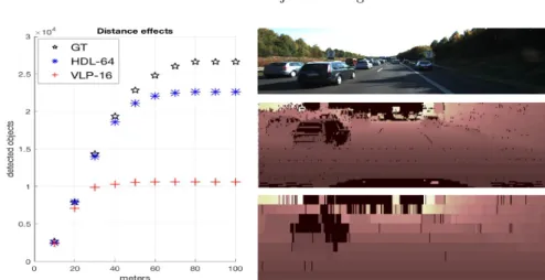
Fig. 2.Left: Vehicle level comparison between total Ground-Truth (GT) objects and True Positives (TP) obtained with both systems using the whole training set filtered at different maximum distances. Right: Kitty training samples exemplifying the scarcity of data of lidar-based methods when compared to image ones. From top to bottom, RGB Camera image, HDL-64 and simulated VLP-16 range images.
case the detector produces the ideal output). Evaluation results of these methods are respectively reported in Table 1, over the full dataset, only the testing set, and only the training set. The geometric-only detector that we set as a baseline for the system, uses the ground removal algorithm described in [20]. Then a clus-tering step is performed along with the bounding box fitting process described in Sec.3.3. Finally, it uses the rectangular fitting error to classify clusters in three different classes:vehicle clusters, which have a low fitting error and are allowed to associate with existing tracks as well as to start new ones; non-vehicle clus-ters, which fitting error exceeds the non-vehicle threshold or whose dimensions are over the allowed size; andpossible vehicle clusters, which fitting error is in between the other two thresholds and consequently are allowed to be associated with existing tracks but not to create new ones.
Table 1.Point-wise vehicle classification modules evaluation
HDL-64 VLP-16
Geometric DeepLidar GT Geometric DeepLidar GT Train Test Test Train Train Test Test Train Mostly Tracked (%) 7.4 10.6 18.5 44.5 0.5 2.2 4.3 5.0 Partly Tracked (%) 56.5 45.1 52.2 47.7 31.4 25.7 37.2 53.2 Mostly Lost (%) 35.9 44.3 29.4 7.8 68.1 72.2 58.5 41.8 Recall (%) 46.4 42.1 55.4 79.0 21.2 15.9 24.8 39.9 Precision (%) 44.1 37.5 63.8 73.9 24.9 18.8 64.2 70.7 MOTA -25.7 -38.9 15.5 41.9 -53.3 -60.0 6.2 15.0
Observing the results, we can conclude that for both sensors the tracking system performs systematically better when our the Deep Lidar module is used as detector, instead of the Geometric approach.
It is noticeable that the MT/PT/ML metrics of the PUCK sensor CNN-detector are closer to the ideal system performance (GT columns) than those obtained with the HDL-64 detector. This is due to the sensor lower resolution that makes distant objects almost undetectable, and suggests that our CNN detector performs very well with PUCK data, and that there is room to improve the detection of far vehicles in our HDL-64 version. The same conclusion holds for the rest of the metrics. This is, relatively to its GT capacities, the PUCK system with the deep detector gets noteworthy values, although those are in general lines low due to the sensor characteristics and its scarce data.
4.2 Detection distance evaluation
We performed different experiments to gain an insight to the maximum detec-tion distance that our low resoludetec-tion system can manage. For this experiments, point-level segmentation ground truth was used in order to decouple the effect of the CNN in the system, filtering at different maximum distances both the track-ing results and the Kitti tracktrack-ing ground truth to exclude from evaluation the objects not present in the selected area. Attending to the results, two distance performance metrics have been defined. On one hand, theeffective detection dis-tance, which we defined as the maximum distance at which the system recall (T P/(T P+F N)) remains over a 90%. On the other hand, themaximum detec-tion distance, a less restrictive measure to obtain the distance at which at least a third of the new vehicles are correctly tracked. To calculate it, we set an incre-mental recall metric (∆T P/(∆T P+∆F N)) that computes the recall with the TP and FN increments produced due to an increase of the distance threshold. Results of these maximum distance experiments are shown on Table 2, where it can be appreciated that systems based on both high-end and low resolution lidar sensors have similar performances in near field. We can also observe that the HDL-64 version achieves a maximum detection distance (incremental recall > 33.3%) of 60 meters and an effective detection distance (recall> 90%) of 40 meters, whereas the simulated VPL-16 low resolution version scores a half in the two metrics, 30 meters of maximum and 20 meters of effective detection distance. This can be clearly appreciated in Fig. 2 (left), which shows the number of true positives and ground truth objects as function of distance for both systems.
5
Conclusions
In this work a low resolution lidar-based vehicle detection and tracking sys-tem has been developed. For the detection task a convolutional neural network has been designed and trained using a decimated version of the Kitti Tracking Benchmark dataset to replicate the geometrics of a Velodyne VLP-16 sensor. The neural network architecture proposed has been successfully verified, achieving a
Table 2.Detection distance evaluation HDL-64 CNN-GT VLP-16 CNN-GT 10m 20m 30m 40m 60m 80m 10m 20m 30m 40m 60m 80m Mostly Tracked (%) 95.7 87.5 80.5 68.7 51.4 45.9 94.3 67.2 18.6 5.8 5.1 5.0 Partly Tracked (%) 3.3 9.4 15.9 26.2 42.1 46.6 3.3 27.1 64.6 64.0 56.6 53.2 Mostly Lost (%) 1.0 3.1 3.5 5.1 6.5 7.5 2.4 5.7 16.8 30.2 38.3 41.8 Recall (%) 99.5 96.5 92.9 90.0 83.4 79.5 99.2 89.8 68.9 53.0 42.8 39.9 Precision (%) 66.3 72.7 73.2 73.1 74.1 74.4 90.6 86.0 79.0 71.7 70.6 70.7 MOTA -26.2 43.4 47.6 46.6 44.9 42.9 73.5 65.3 40.2 21.2 16.2 15.0 Inc. Rec 99.5 95.2 88.5 82.2 44.0 25.5 99.2 85.6 43.1 8.0 2.4 0.0
precision of 69.3% and a recall of 78.8% in a two-classes (vehicle / non-vehicle) point-wise level classification problem, while using low resolution data that rep-resents only a 0.5% of the data present in one single Kitti RGB image. The Kitti Tracking Benchmark results show that the CNN-based detection module im-proves systematically the whole system performance, measured at vehicle level, in all the analyzed metrics. We show that, despite having shorter detection dis-tance, in near field our low resolution system achieves similar performance to the high-end version, while the sensor cost is reduced by an order of magnitude.
References
1. Abualhoul, M.Y., Merdrignac, P., Shagdar, O., Nashashibi, F.: Study and evalua-tion of laser-based percepevalua-tion and light communicaevalua-tion for a platoon of autonomous vehicles. In: Intell. Transp. Syst. (ITSC), 2016 IEEE 19th Int. Conf. on, pp. 1798– 1804. IEEE (2016)
2. Arras, K.O., Mozos, O.M., Burgard, W.: Using boosted features for the detection of people in 2d range data. In: Robotics and Autom., 2007 IEEE Int. Conf. on, pp. 3402–3407. IEEE (2007)
3. Behley, J., Steinhage, V., Cremers, A.B.: Performance of histogram descriptors for the classification of 3d laser range data in urban environments. In: Robotics and Autom. (ICRA), 2012 IEEE Int. Conf. on, pp. 4391–4398. IEEE (2012)
4. Bernardin, K., Stiefelhagen, R.: Evaluating multiple object tracking performance: the clear mot metrics. EURASIP J. on Image and Video Process.2008(1), 246,309 (2008)
5. Chen, X., Ma, H., Wan, J., Li, B., Xia, T.: Multi-view 3d object detection network for autonomous driving. arXiv preprint arXiv:1611.07759 (2016)
6. Douillard, B., Underwood, J., Kuntz, N., Vlaskine, V., Quadros, A., Morton, P., Frenkel, A.: On the segmentation of 3d lidar point clouds. In: Robotics and Autom. (ICRA), 2011 IEEE Int. Conf. on, pp. 2798–2805. IEEE (2011)
7. Eidehall, A., Pohl, J., Gustafsson, F., Ekmark, J.: Toward autonomous collision avoidance by steering. IEEE Transactions on Intell. Transp. Syst. 8(1), 84–94 (2007)
8. Engelcke, M., Rao, D., Wang, D.Z., Tong, C.H., Posner, I.: Vote3deep: Fast object detection in 3d point clouds using efficient convolutional neural networks. In: Robotics and Autom. (ICRA), 2017 IEEE Int. Conf. on, pp. 1355–1361. IEEE (2017)
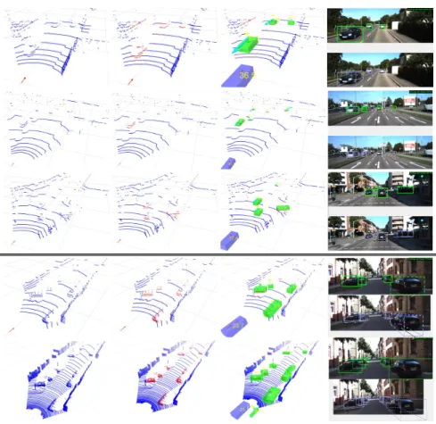
Fig. 3.Qualitative results. In columns, images show the raw input, the Deep detector output with vehicle points in red, the final tracked vehicles and the RGB projected bounding boxes submitted for evaluation. The first three rows illustrate different PUCK results, while the fourth and fifth are a comparison between the simulated VLP-16 and the HDL-64 resolution systems. As can be seen, near field performances are similar, but the PUCK detection distance is shorter.
9. Geiger, A., Lenz, P., Urtasun, R.: Are we ready for autonomous driving? the kitti vision benchmark suite. In: Comput. Vis. and Pattern Recognit. (CVPR), 2012 IEEE Conf. on, pp. 3354–3361. IEEE (2012)
10. Graham, B.: Sparse 3d convolutional neural networks. arXiv preprint arXiv:1505.02890 (2015)
11. He, K., Zhang, X., Ren, S., Sun, J.: Deep residual learning for image recognition. In: Proc. of the IEEE conf. on comput. vis. and pattern recognit., pp. 770–778 (2016)
12. Kohlhaas, R., Schamm, T., Lenk, D., Z¨ollner, J.M.: Towards driving autonomously: Autonomous cruise control in urban environments. In: Intell. Vehicles Symposium (IV), 2013 IEEE, pp. 116–121. IEEE (2013)
13. Krizhevsky, A., Sutskever, I., Hinton, G.E.: Imagenet classification with deep con-volutional neural networks. In: Adv. in neural inf. process. syst. (NIPS), pp. 1097–
1105 (2012)
14. Li, B.: 3d fully convolutional network for vehicle detection in point cloud. arXiv preprint arXiv:1611.08069 (2016)
15. Li, B., Zhang, T., Xia, T.: Vehicle detection from 3d lidar using fully convolutional network. arXiv preprint arXiv:1608.07916 (2016)
16. Li, Y., Huang, C., Nevatia, R.: Learning to associate: Hybridboosted multi-target tracker for crowded scene. In: Comput. Vis. and Pattern Recognit., 2009. CVPR 2009. IEEE Conf. on, pp. 2953–2960. IEEE (2009)
17. Long, J., Shelhamer, E., Darrell, T.: Fully convolutional networks for semantic segmentation. In: Proc. of the IEEE Conf. on Comput. Vis. and Pattern Recognit., pp. 3431–3440 (2015)
18. Mertz, C., Navarro-Serment, L.E., MacLachlan, R., Rybski, P., Steinfeld, A., Suppe, A., Urmson, C., Vandapel, N., Hebert, M., Thorpe, C., et al.: Moving object detection with laser scanners. J. of Field Robotics30(1), 17–43 (2013) 19. Papon, J., Abramov, A., Schoeler, M., Worgotter, F.: Voxel cloud connectivity
segmentation-supervoxels for point clouds. In: Proc. of the IEEE Conf. on Comput. Vis. and Pattern Recognit. (CVPR), pp. 2027–2034 (2013)
20. Petrovskaya, A., Thrun, S.: Model based vehicle detection and tracking for au-tonomous urban driving. Auau-tonomous Robots26(2-3), 123–139 (2009)
21. Rekleitis, I., Bedwani, J.L., Dupuis, E.: Autonomous planetary exploration using lidar data. In: Robotics and Autom., 2009. ICRA’09. IEEE Int. Conf. on, pp. 3025–3030. IEEE (2009)
22. Ren, S., He, K., Girshick, R., Sun, J.: Faster r-cnn: Towards real-time object de-tection with region proposal networks. In: Adv. in neural inf. process. syst., pp. 91–99 (2015)
23. Sermanet, P., Eigen, D., Zhang, X., Mathieu, M., Fergus, R., LeCun, Y.: Overfeat: Integrated recognition, localization and detection using convolutional networks. arXiv preprint arXiv:1312.6229 (2013)
24. Teichman, A., Levinson, J., Thrun, S.: Towards 3d object recognition via classi-fication of arbitrary object tracks. In: Robotics and Autom. (ICRA), 2011 IEEE Int. Conf. on, pp. 4034–4041. IEEE (2011)
25. Triebel, R., Shin, J., Siegwart, R.: Segmentation and unsupervised part-based dis-covery of repetitive objects (2010)
26. Vaquero, V., del Pino, I., Moreno-Noguer, F., Sol`a, J., Sanfeliu, A., Juan, A.C.: Deconvolutional networks for point-cloud vehicle detection and tracking in driving scenarios. In: Mobile Robotics, 2017. (ECMR-2017). Eur. Conf. on. IEEE (2017) 27. Vaquero, V., Repiso, E., Sanfeliu, A., Vissers, J., Kwakkernaat, M.: Low cost,
robust and real time system for detecting and tracking moving objects to automate cargo handling in port terminals. In: Robot 2015: 2nd Iber. Robotics Conf., pp. 491–502. Springer (2016)
28. Wan, L., Raksincharoensak, P., Maeda, K., Nagai, M.: Lane change behavior mod-eling for autonomous vehicles based on surroundings recognition. Int. J. of Auto-mot. Eng.2(2), 7–12 (2011)
29. Wang, D.Z., Posner, I.: Voting for voting in online point cloud object detection. In: Robotics: Science and Syst. (2015)
30. Wang, D.Z., Posner, I., Newman, P.: What could move? finding cars, pedestrians and bicyclists in 3d laser data. In: Robotics and Autom. (ICRA), 2012 IEEE Int. Conf. on, pp. 4038–4044. IEEE (2012)
31. Wang, Z., Kulik, L., Ramamohanarao, K.: Proactive traffic merging strategies for sensor-enabled cars. In: Proc. of the fourth ACM int. workshop on Vehicular ad hoc networks, pp. 39–48. ACM (2007)