Micro Application Example

(1)

Closed-Loop Positioning Control

with standard Drives

(2)

V2.0 16.07.2008 2/54 C opyr ight © Si em ens AG 2 008 Al l r ights r e se rv ed Set0 1_D ocT e ch_ 2d0 _en.d o c

Note

The Micro Automation Sets are not binding and do not claim to be complete regarding the circuits shown, equipping and any eventuality. The Micro Automation Sets do not represent customer-specific solutions. They are only intended to provide support for typical applications. You are responsible for ensuring that the described products are correctly used. These Micro Automation Sets do not relieve you of the responsibility of safely and professionally using, installing, operating and servicing equipment. When using these Micro Automation Sets, you recognize that Siemens cannot be made liable for any damage/claims beyond the liability clause described. We reserve the right to make changes to these Micro Automation Sets at any time without prior notice. If there are any deviations between the recommendations provided in these Micro Automation Sets and other Siemens publications – e.g. Catalogs – the contents of the other documents have priority.

Warranty, liability and support

We do not accept any liability for the information contained in this document. Any claims against us – based on whatever legal reason – resulting from the use of the examples, information, programs, engineering and performance data etc., described in this Micro Automation Set shall be excluded. Such an exclusion shall not apply in the case of mandatory liability, e.g. under the German Product Liability Act (“Produkthaftungsgesetz”), in case of intent, gross negligence, or injury of life, body or health, guarantee for the quality of a product, fraudulent concealment of a deficiency or breach of a condition which goes to the root of the contract (“wesentliche Vertragspflichten”). However, claims arising from a breach of a condition which goes to the root of the contract shall be limited to the foreseeable damage which is intrinsic to the contract, unless caused by intent or gross negligence or based on mandatory liability for injury of life, body or health. The above provisions does not imply a change in the burden of proof to your detriment.

Copyright© 2008 Siemens IA and DT. It is not permissible to transfer or copy these Micro Automation Sets or excerpts of them without first having prior authorization from Siemens IA and DT in writing.

(3)

Foreword

Micro Automation Sets are functional and tested automation configurations based on IA/DT standard products for easy, fast and inexpensive

implementation of automation tasks for small-scale automation. Each of the available Micro Automatic Sets covers a frequently occurring subtask of a typical customer problem in the lower performance range.

The sets help you obtain answers with regard to required products and the question how they function when combined.

However, depending on the system requirements, a variety of other components (e.g. other CPUs, power supplies, etc.) can be used to implement the functionality on which this set is based. For these

components, please refer to the respective SIEMENS IA and DT catalogs. The Micro Automation Sets are also available at:

(4)

1 Fields of Application and Benefits

1.1 Automation

problem

A wire cutting machine is to produce a customer-specific number of wire rods with customized length.

After equipping the machine with the desired wire-wound coil, the management of the coil’s type and available capacity is to be

voltage-protected, the positioning axis unwinds the desired length from the wire-wound coil and cuts the wire. This operation is repeated according to the number entered together with a production ID.

After completing the production job, voltage-resistant buffering has to be performed for all specific production data to read it from a PC once a day and to archive them there within the scope of quality assurance.

After feeding in the wire prior to production, the wire is to be located in front of the cutting device.

Figure 1-1

Type2 Type3 Type1

(6)

1.2 Automation solution – Set 1

With the aid of the TP177micro Touch Panel, all material data of the available wire-wound coils that is relevant to the production can be stored as a recipe in the voltage-resistant memory module of the S7-200 CPU 224XP. The following information is stored under the designation of the wire-wound coil:

• Wire size

• Length of the pieces of wire to be cut of the corresponding job

• Material capacity of the wire-wound coil (initial value)

• Production ID of the job (initial value)

Prior to production, the wire-wound coil to be used for the production has to be selected via the TP177micro Touch Panel.

While feeding in the wire, a block that runs in the S7-200 CPU 224XP controls the G110 frequency inverter via the analog interface in such a way that the wire comes to a standstill after passing an inductive sensor and that the positioning axis is thus homed.

An HTL encoder reports the traveled distance of the axis to the S7-200 CPU 224XP in the form of pulses.

After entering the production ID and the number of pieces of wire to be produced using the TP177micro Touch Panel, a block running in the S7-200 CPU 224XP causes the frequency inverter to move the positioning axis by the desired wire length. Via a digital output signal, the S7-200 CPU 224XP subsequently controls a cutting device that cuts the wire.

This operation is repeated according to the entered number. After completion or premature termination of the job the following production parameters are stored in the voltage-resistant memory module of the S7-200 CPU 224XP.

• Time and date stamp of the production job

• Diameters of the wire rods

• Length of the pieces of wire

• Quantity of the residual material on the coil

• A unique production ID for the job

• Actual number of cut wire rods

The thus buffered information can be read out via a serial link, for instance with the aid of a PC/PPI cable and the S7-200 Explorer STEP7 Micro/WIN tool and stored as a csv file.

When selecting a new wire-wound coil via the TP177micro Touch Panel, the remaining capacity of the previous coil that has been permanently updated during production is written to the recipe of the relevant material

(7)

data. Since the recipe is also stored in the voltage-resistant memory module of the S7-200 CPU 224XP, the remaining capacity of the old wire-wound coil is again available when it is reused in the cutting device. If the remaining capacity of the wire-wound coil falls below a specific value, a warning is displayed on the TP 177micro Touch Panel. And if the amount of wire is not sufficient for the planned job, the entered number of wire rods is reduced to the possible number and this fact is also reported via the TP.

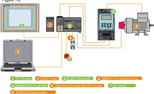
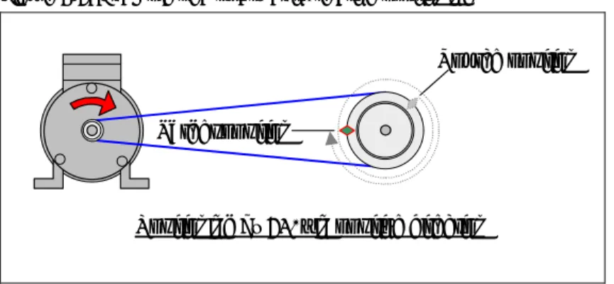
Figure 1-2 6 4 8 5 3 2 1 s H zH z 1234567891 0 O N 123 P F M J O G s SIMATIC PANEL TO U C H TP 177 micro S7-200 CPU 224XP SINAMICS G110 with BOP Asynchronous motor with HTL encoder

LOGO! Power SIMATIC PXI inductive sensor

1 2 3 4 5 6 7NC contact 7 s WINDOWS-based system 8

(8)

1.3 Fields of application

The Micro Automation Set is particularly suitable for industrial applications requiring the positioning of objects. The product combination in conjunction with the software library enables a cost-effective positioning solution, for example, in the following applications:

• Cutters, for example, for pipes

• Conveyors • Feeders • Lifting stages • Rotary tables • Hoisting devices

1.4 Benefits

• Simple solution for positioning a linear axis (horizontally or vertically) or a rotary axis.

• Clearly reduced engineering overhead by providing a command library for STEP 7 Micro/WIN.

• The use of a particularly sturdy control algorithm ensures that a manual optimization of the position control is not necessary even if there are strong load fluctuations.

• Realization of the drive task without comprehensive control engineering know-how. The SIMATIC S7-200 takes the position control.

• Engineering and commissioning of the S7-200 and the position controller with only one software tool: STEP 7 Micro/WIN.

• Cost-effective and high-performance solution with SINAMICS G110.

• In addition to your control problem, the S7-200 can also solve multiple automation problems.

• Visualization and control of the process via the TP 177micro Touch Panel.

(9)

2 Configuration

Connection diagram Figure 2-1 L1 N PE L1 L2 L3 U1 V1 W1 1 2 3 4 5 6 7 8 9 10 1M 0.0 0.1 0.2 0.3 0.4 0.5 0.6 0.7 2M 1.0 1.1 1.2 1.3 1.4 1.5 M L+ 1M 1L+ 0.0 0.1 0.2 0.3 0.4 0.5 2M 2L+ 0.5 0.6 0.7 1.0 1.1 PE M L+ M I V M +A +B L+ M L+ M 2 3 1 wht blu red blk Connector of the encoder cable

contact side (not solder side)

1 2 PR O F IB US c abl e PC /P PI o r US B /P P I c abl e

WINDOWS-based system for configuring and data archiving

A B K J H M G F E D C L SIMATIC S7-200 – inputs:

Via the preassembled encoder cable, the rotary pulse encoder is connected to the HSC4 high-speed counter that uses the I0.3 and I0.4 inputs. The D-sub connector of the encoder cable was removed.

The signal cable of the inductive sensor is connected to I0.6. I0.0 was used for the OFF button.

SIMATIC S7-200 – outputs:

The inverter with analog input receives its frequency setpoint via the analog voltage output of the controller (terminals M, V). A shielded cable has to be used. On the inverter, the analog signal is applied to terminal 9 and the associated analog reference ground is applied to terminal 10 of the signal interface. The analog reference ground and the ground of the 24V supply are jumpered on the inverter (terminals 7, 10).

(10)

The “start motor” command is applied at digital output Q1.0 of the controller. It is connected to terminal 3 of the inverter’s signal interface. The “reversal” signal is applied at digital output Q1.1 of the controller. It is connected to terminal 4 of the inverter’s signal interface.

SINAMICS G110 frequency inverter

In primary circuit, the connection of the frequency inverter to the 230V mains is a single-phase connection.

The asynchronous motor operated in delta connection is connected in secondary circuit.

NOTICE _{Please observe that the phase angle of the encoder pulses A and B}

correlates with the phase angle L1, L2 and L3 of the motor supply. If correct positioning is not possible, the problem can possibly be solved by reversing the encoder tracks or two motor phases. If the motor does not run in the desired direction, encoder tracks and two motor phases have to be reversed.

24V supply

The 24VDC power supply of the devices is provided by a LOGO! Power 1.3A.

Protection

(11)

3 Hardware and Software Components

Products

Table 3-1

Component No. MLFB / order number Note

RCBO 1 5SU1154-7KK06

LOGO! Power 24V/1.3A 1 6EP1331-1SH02

SIMATIC S7-200 (CPU

224XP) 1 6ES7214-2BD23-0XB0

TP 177micro Touch Panel 1 6AV6640-0CA11-0AX0 SINAMICS G110, frequency

inverter

6SL3211-0AB12-5UA1 SINAMICS G110, frequency

inverter with integrated EMC filter

1

6SL3211-0AB12-5BA1 Alternatively

Low-voltage asynchronous

motor 1 1LA7070-4AB10-Z H57 Motor with rotary pulse encoder, 1024 pulses per revolution Encoder cable

for rotary pulse encoder 1 6SX7002-0AN30-1AC0 Remove D-sub connector! SIMATIC PXI350

INDUCTIVE SENSOR 40X40MM

1 3RG4141-3AB01

Pushbutton, red, 1NC 1 3SB3203-0AA21

MC 291 MEMORY

MODULE, 256 KBYTES 1 6ES7291-8GH23-0XA0

Accessories

Table 3-2

Basic Operator Panel (BOP)

(12)

V2.0 16.07.2008 12/54 C opyr ight © Si em ens AG 2 008 Al l r ights r e se rv ed Set0 1_D ocT e ch_ 2d0 _en.d o c Configuration software/tools Table 3-3

WinCC flexible micro 1 6AV6610-0AA01-2CA8

Step 7 Micro/Win 1 6ES7810-2CC03-0YX0

PC/PPI cable 6ES7901-3CB30-0XA0

USB/PPI cable 1 6ES7901-3DB30-0XA0

Alternatively; can also be used for loading the TP177 micro SINAMICS MICROMASTER

(13)

4 Principle of Operation

4.1 Introduction to positioning

What does “closed-loop controlled positioning” mean?

In the context of this application, the following definitions can be provided: When “positioning”, an electrically driven component of a device or plant approaches a defined local point or angle by means of a linear or rotary motion or the component is moved by the distance Δs or the angle Δφ. When the positioning is “closed-loop controlled”, the motion is performed in a closed control loop in which path and velocity (motor speed) are the controlled variables. The disturbance variables are differing load torques. The SIMATIC S7-200 transfers the “velocity” controller output to the

frequency inverter as an analog voltage that is interpreted by the frequency inverter as a setpoint frequency according to its parameterized V/f

characteristic. Considering the slip of the asynchronous motor depending on the load torque, a specific speed is set. According to this speed, the component to be positioned travels a smaller or larger number of path or angle increments. They are detected by the rotary pulse encoder that is located directly on the motor shaft and supplied to the controller via its high-speed counter inputs.

From this information and including the setpoint values “position”,

“positioning speed” and “acceleration (torque)”, a control algorithm counting the encoder pulses calculates the necessary “velocity” controller output. This results in a velocity profile whose processing finally leads to an exact positioning. Figure 4-1 Controller Controlled system Frequency inverter, asynchronous motor Position Velocity

Acceleration (torque) Analog value0 – 10V

Manipulated value Reference variable Load torque Disturbance variable Controlled variable Position Velocity Encoder pulses Control with MicroPos blocks

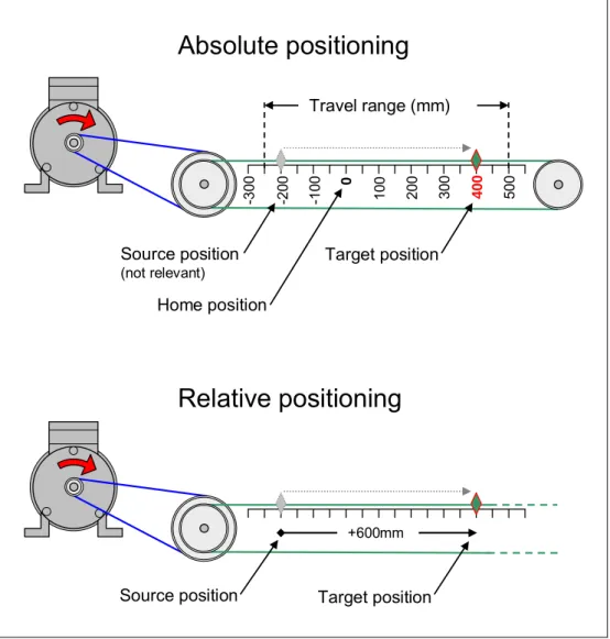
What is the difference between absolute and relative positioning?

When absolute positioning is used, you directly specify the target position to be approached. When relative positioning is used, you enter a path length by which the component is to be moved.

(14)

To enable absolute positioning, it is required that the zero point of your travel path (home position) be defined once in advance. The counter with which the pulses of the rotary pulse encoder are counted is adjusted to the position of the physical axis, .i.e. it is set to a defined value (preferably 0) at a defined local point. Homing is not necessary for relative positioning. Figure 4-2: Example of absolute/relative positioning

0 -10 0 -20 0 10 0 20 0 -30 0 30 0 40 0 50 0 Travel range (mm) Home position Target position Source position (not relevant)

Absolute positioning

Target position +600mm Source position

Relative positioning

What is the difference between a linear and a rotary axis?

• Linear axis:

A linear axis is particularly suitable for linear motions in the horizontal or vertical plane. For the distance traveled during positioning, the blocks assume the “length” dimension. Depending on the velocity or ratios of dimensions, the user applies the corresponding parameters (position, velocity, etc.), for example, to mm, cm or inch.

(15)

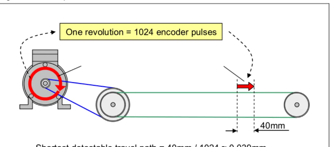
An important parameter of the linear axis is the correlation between the physical variable “distance traveled” and a motor or rotary pulse

encoder revolution. The parameter thus considers gear, belt, spindles, etc. that eventually convert the rotary motion to a linear motion. Figure 4-3: Example of a linear axis, distance traveled

One revolution = 1024 encoder pulses

40mm

Shortest detectable travel path = 40mm / 1024 ≈0.039mm

The Map_Ind_Lin library is used for the linear axis. The names of all

blocks have “Lin_” as a prefix.

• Rotary axis:

The rotary axis – also referred to as a “modulo axis” – designates a type of positioning where a rotary motion is repeated after each completed motional sequence. Taking this fact into account, the position value of the drive-end, moved component is specified in angular degrees 0 ≤φ < 360.0 and reset to 0 after each “rotation”.

For the unique detection of the absolute position, the rotary axis additionally features a rotation counter that is adjusted each time the axis is moved – irrespective of whether the positioning is absolute or relative or whether the rotary axis is moved in jog mode. Without homing, the rotation counter is set to 0 when restarting the controller. With homing, the rotation counter is set to a value that corresponds to the specified reference angle.

If you specify, for instance, an angle of +740° for the physical local point x0 when homing, the rotation counter has the value +2 in x0.

An important parameter of the rotary axis is the correlation between the physical variable “angle traveled” and a motor or rotary pulse encoder revolution. The parameter thus considers gear, belt, spindles, etc. that finally represent the ratio.

(16)

Figure 4-4: Example of a rotary axis, angle traveled

One motor revolution = 1024 encoder pulses

Smallest detectable angle of revolution

= 28° / 1024 ≈1′38″

φ= 28°

The following specifics have to be considered for a rotary axis:

– Absolute positioning with preset direction of rotation

At the drive end, the target position has to be approachable with a maximum of one “rotation” (φ < 360.0°). Larger angle settings cause a termination of the job. Negative angle settings are also not

permissible. The direction of rotation is to be specified by an – compared to a linear axis – additional direction parameter. Figure 4-5: Example of a rotary axis, absolute positioning

Home position _{Source position}

Target position

Positioning to 270° in negative direction

0°

Home position _{Source position}

Target position

Positioning to 270° in positive direction

0°

– Absolute positioning on the shortest path

(17)

calculates the shortest path to the target and selects the direction of rotation accordingly.

– Relative positioning

Both angle settings > 360.0° and negative angles are possible. Figure 4-6: Example of a rotary axis, relative positioning

Source position Target position

Positioning by 630° in positive direction

The Map_Ind_Rot library is used for the rotary axis. The names of all

blocks have “Rot_” as a prefix.

What is a travel profile?

Depending on the purpose, travel profiles describe various characteristics (path, velocity, acceleration, moment, power, etc.) that describe a desired motional sequence. The time or the path is mostly plotted on the abscissa. The following applies to a positioning operation by means of the MAP Ind blocks:

• Acceleration is always performed from zero and the component is always decelerated to a standstill.

• The steepness of acceleration ramp and deceleration ramp is identical

• The controlled variable for the required acceleration/deceleration is the moment.

(18)

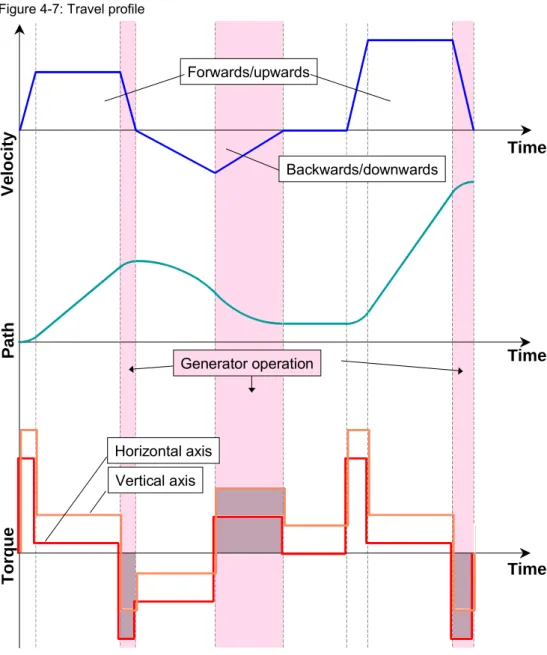
Figure 4-7: Travel profile

Veloci ty _Time Path _Time Forwards/upwards Backwards/downwards Torque Time Horizontal axis Vertical axis Generator operation

For system optimization, the two “MAP_Ind_...” libraries offer a

“…_Com_Monitor” block with which alternatively the dependencies M(t),

v(t) and s(t) can be displayed as travel profiles in STEP 7 MicroWin.

What is the difference between a horizontal and a vertical axis?

While the “horizontal axis” merely requires that the forces of

acceleration/deceleration and the friction forces be considered parallel to the direction of motion for a mass to be moved, the gravitational force of the mass to be moved has to be additionally considered for the vertical axis. This requires the provision of a larger torque from the inverter to achieve the same accelerating/decelerating torques as for the horizontal axis. Figure 4-7 shows a qualitative representation of the torque

(19)

Under which circumstances does the motor become the generator?

Whenever energy stored in the system is to be degraded, the motor becomes the generator. The following energies have to be mentioned:

• Potential energy

(due to a suspended load)

• Kinetic energy

(due to moving masses)

Energy released when lowering a load or decelerating a flywheel that would drive the motor from the mechanical end has to be degraded by the inverter as power loss. The inverter copes with smaller powers without additional measures. Larger powers require braking resistors or power recovery has to be provided. Figure 4-7 shows the time intervals of generator operation. The hatched areas under the torque characteristics are proportional to the energy to be degraded.

4.2 Block libraries for moving

linear and rotary axes

Overview of available positioning blocks

Figure 4-8 Lin_Init_horizontal Lin_Init_vertical Lin_MoveJog Lin_Home Lin_MoveAbs Lin_MoveRel Lin_StopMotion Rot_Init Rot_MoveJog Rot_Home Rot_MoveAbs Rot_MoveRel Rot_StopMotion Lin_Com_Monitor Rot_Com_Monitor Lin_Control Rot_Control MAP_Ind_Lin library for linear axis

MAP_Ind_Rot library for rotary axis

The library description also included in Micro Automation Set 1 provides a detailed block description. The MAP_Ind_Lin library for linear axes is used

(20)

Task of the “Lin_Init_horizontal” block

This application describes a horizontal material transport. For this reason, the “Lin_Init_horizontal” block is used here. The initialization block

combines those input and output parameters that refer, so to speak, to all further blocks of the library and that are used by the positioning’s control algorithm. Furthermore, the user-specific units of measurement are standardized in this block.

Motor characteristics, absolute upper limits for velocity and torque1_{and the}

transfer factor indicating which feed corresponds to the linear motion of a motor revolution are mainly entered in “Lin_Init_horizontal”.

“Lin_Init_horizontal” has to be processed once before the remaining blocks – which have to be called cyclically – are executed for the first time. Trigger “Lin_Init_horizontal” with SM0.1.

Task of the “Lin_MoveJog” block

Using the “Lin_MoveJog” block, you realize manual mode. The block features two bit inputs for jog mode (“JogPos” and “JogNeg”).

Accelerating/decelerating torque and a limit velocity can be parameterized at the block.

Task of the “Lin_Home” block

To enable absolute positioning, the three-dimensional travel path has to be synchronized with the controller’s position counter. This is achieved by assigning a specific value to a defined point of your travel path (= home position). This is done during runtime of the automation program. “Lin_Home” offers two referencing variants:

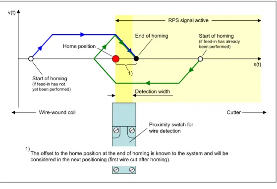
• Searching for the home position

For searching the motor is started with “Execute” block parameter =1 and the required direction of rotation (“Direction” parameter = ±1). If the moving component is detected by a sensor at the user-defined home position (“RPS” signal), a specific reference value (“Home_Position”) is assigned to the current position with this event. The detection of the sensor is performed via its positive or negative edge. The sensor can, for example, be an inductive proximity switch or a photoelectric barrier. Your user program has to be designed in such a way that the sensor is always approached from the same direction when homing to eliminate its detection width.

In this “wire cutting machine” application example, homing is performed when feeding in the wire or before the first cutting operation as shown in the graphic representation below. The distance “proximity switch – cutter” (with minus sign) is entered as a position value of the home

1_{Upper limits are not even exceeded during operation if higher values are parameterized in the} blocks initiating a motion.

(21)

position. Thus the current wire position = 0mm if the wire tip is located exactly at the cutter.

Figure 4-9: Home position search

Wire-wound coil Cutter

Proximity switch for wire detection Detection width v(t) s(t) Home position RPS signal active Start of homing

(if feed-in has already been performed)

Start of homing

(if feed-in has not yet been performed)

End of homing

1)

The offset to the home position at the end of homing is known to the system and will be considered in the next positioning (first wire cut after homing).

1)

• Setting the home position.

When setting the home position, the motor is stopped. 0 has to be specified for the “Direction” block parameter. If the block detects a positive edge at “Execute”=1 at the “RPS” input parameter, the current position is set to a parameterizable reference value (“Home_Position”). In the “wire cutting machine” application example described in this document, the home position is set to the value 0 whenever the wire tip is located exactly at the cutter after a completed wire cut.

For the home position search, accelerating/decelerating torque and a limit velocity can be parameterized at the block.

Task of the “Lin_MoveAbs” block

Initiated by a positive edge at the “Execute” input parameter, the motor starts from the current position for a closed-loop-controlled approach to the end point specified via the “Position” input parameter. A prerequisite for absolute positioning is previous homing with the “Lin_Home” block.

(22)

Task of the “Lin_MoveRel” block

Initiated by a positive edge at the “Execute” input parameter, the motor starts at the current position to approach the point whose distance from the starting point is specified by the “Distance” input parameter on a closed-loop-controlled basis. Previous homing using the “Lin_Home” block is not required in this case.

Task of the “Lin_StopMotion” block

“Lin_StopMotion” is used to stop a currently active motion – irrespectively of the specific MAP Ind block that triggered it. The block offers two variants for stopping:

• Stopping via the “AUS3” inverter digital input.

The steepness of the deceleration ramp is set when parameterizing the inverter. The stop is triggered by a positive edge at the “Execute_Off3” input parameter.

• Stopping via the “Lin_StopMotion” block.

This variant is used in this application. The steepness of the

deceleration ramp is set by the “Decel_Torque_Ramp” input parameter of the block. The stop is triggered by a positive edge at the

“Execute_Ramp” input parameter.

It is not only possible to use both variants for stopping alternatively, they can also be used together in one program.

The block monitors the deceleration times (separate monitoring of both variants for stopping). The upper limits can be parameterized. When the limits are violated, the “Time_Exceeded” output bit parameter is set.

Task of the “Lin_Control” block

• The block uses a status word to inform the user on all system states and limit value violations:

– Motor stopped

– Maximum moment reached

– Axis not synchronized

– Pulse counter overflow

– Direction conflict (rotary pulse encoder ↔ motor phase angle)

– Following error exceeded

– System not initialized

• The value of the current position is available to the user in the “Act_Position” output parameter.

(23)

• Whenever the motor is stopped from the perspective of the MAP Ind blocks, a “Brake” bit output is set to a logic “1”. For example, a holding brake or the pulse enable for the inverter can then be controlled.

Task of the “Lin_ComMonitor” block

In the commissioning phase the “Lin_ComMonitor” block supports the user in optimizing the dynamic response. The block alternatively records

(parameterizable)

• moment

• velocity

• position

in real time to be able to subsequently represent their time characteristics in the STEP7 Micro/Win trend display.

A positive edge at the “Start” bit input parameter starts the recording. Where the data is to be stored is communicated to the block via the

“pTableStart” input parameter by means of a pointer. The block records 249 REAL values in the 8ms grid. In the trend display, subsequently view the “Out” output parameter of the block.

Note A parameter description of the MAP Ind blocks is available not only in the library description of this Micro Automation Set, but also in STEP7

Micro/WIN directly as a comment in the relevant protected MicroPos block.

4.3 Configuring the G110 frequency inverter

Parameterization steps

Due to the universality of the SINAMICS frequency inverters, the adaptation to a specific application requires that the inverter be parameterized. This setting procedure is facilitated by the fact that many applications can be operated with the factory default settings if quick commissioning has

previously been performed. If the condition at delivery from the plant of the inverter you are using has been changed, it can be reset to the factory default settings without difficulty. If quick commissioning is set, only the parameters whose adaptation is absolutely necessary can be selected during the parameterization. To meet the specific requirements of this application, application-specific parameterizations are necessary after

the reset to factory default settings and after quick commissioning. Finally,

save the values to the EEPROM of the inverter and, if necessary, save

the entire parameterization to the BOP. This enables you to reload the

parameters to the inverter at any time if required without having to reenter them or to transfer the parameters to other identical inverters.

(24)

To parameterize the inverter, we recommend the following procedure: Table 4-1

No. Step

1. Resetting to factory default settings (if condition at delivery from the plant has been changed)

2. Quick commissioning.

3. Application-specific parameterizations. 4. Saving parameters to the inverter’s EEPROM. 5. Transferring parameter set to BOP for reuse.

Changing parameters

All steps listed above are merely sequences of parameter settings. They can be performed, for example, using the Basic Operator Panel (BOP) that is simply plugged onto the inverter2_.

Figure 4-10

To change a parameter via the BOP, proceed as follows:

(25)

No. Operator input sequence step Note

1. Go to parameterization mode. 2. Select the parameter to be changed.

3. Display the parameter value. 4. Change the parameter value.

When you press FN, you can change each decade individually. 5. Apply the value.

These operations have to be performed for each parameter.

6. Select the display (0000).

7. Exit parameterization mode.

Documents for the SINAMICS G110

The following documents are available for the SINAMICS G110: Table 4-2

Document ID number:

Getting Started Guide 21696936 Operating Instructions 22102965

Parameter List 20977026

4.4 Optimizing the positioning operation

4.4.1 Optimization with regard to the moment of inertia

Relating to all MAP Ind blocks, the Inertia parameter (moment of inertia)

influencing the system dynamics that cannot be easily deduced from motor catalogs or mechanical system requirements like all other input values can be either calculated or determined empirically. The calculation of the moment of inertia of the entire moved system component required by the Lin_Init_horizontal block as an input parameter is difficult. The following sections describe a way to determine the moment of inertia empirically.

(26)

Start value for the moment of inertia

Experience has shown that the tenfold mass inertia of the motor is a good start value. Before commissioning, enter this value for the Inertia parameter at the Lin_Init_horizontal block. For the motor’s mass inertia, please refer to the motor catalog. Accordingly, a value of 0.00052kgm2_{results for the}

motor from Table 3-1.

Optimization process with the aid of the “Lin_ComMonitor” block

To assess the dynamic response of your system, the graphical

representations of the trend curves v(t) and s(t) are alternatively suitable. Consider in particular the end of the positioning operation. If the moment of inertia is set optimally (Figure 4-12), neither distinctive overshoot

(Figure 4-11) nor a “gradual vanishing” (Figure 4-13) of the corresponding curve should occur.

Figure 4-11 v(t) s(t) Overshoot! Overshoot! Figure 4-12 v(t) s(t) Optimum characteristic Optimum characteristic

(27)

V2.0 16.07.2008 27/54 C opyr ight © Si em ens AG 2 008 Al l r ights r e se rv ed Set0 1_D ocT e ch_ 2d0 _en.d o c Figure 4-13 v(t) s(t) Gradual vanishing! Gradual vanishing!

The time characteristic v(t) is also suitable for controlling or optimizing the velocity. It shows whether the velocity parameterized at the relevant block is actually reached.

4.4.2 Optimization of the travel profile

The travel profile is essentially defined by the technological application and an energetic optimization. Determining factors are

• the time within which the positioning operation has to be completed,

• acceleration and deceleration whose upper limits are determined by the motor performance, the application’s mechanical system and the actual process and

• the power demand of the application.

The travel profile can be adjusted to the application as follows: Figure 4-14

t v(t)

Slope is determined by... • rated torque of the motor

•Accel_Torqueor Torque_Limitblock parameter (0...200%)

Maximum velocity is determined by...

(28)

The absolute maximum velocity of the linearly moved component eventually depends on the rated speed relating to the motor frequency. Since the 4-pole motor of this application can be controlled by the inverter with a maximum of 100Hz, its highest speed is 2700 min-1_{. This speed –}

converted to the linear motion of the application – results in the maximum velocity that can be limited with the Velocity_Limit parameter.

The Accel_Torque or Torque_Limit block parameters for limiting the motor torque are indicated as percentages of the rated torque. A torque of up to 200% can be used for a 4-pole motor.

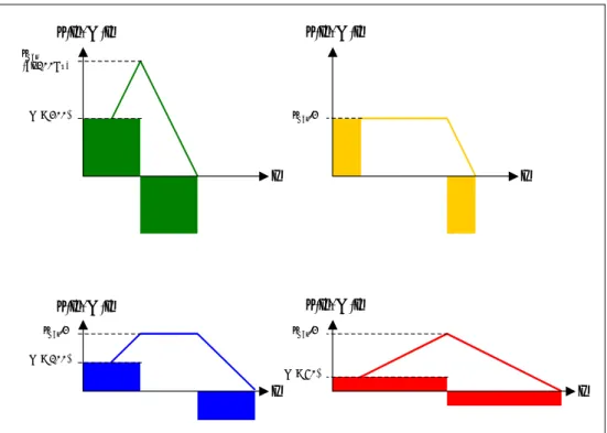
The example in the figure below shows four possible travel profiles that all position over the same distance, i.e. the integrals over the curves v(t) from the starting point to the end point of the motion are identical. Friction losses are negligible.

Figure 4-15: Different travel profiles for the same positioning

t t t v(t), M(t) v(t), M(t) v(t), M(t) t v(t), M(t) M = 200% vmax (at 100Hz) vmax/2 M = 100% vmax/2 vmax/2 M = 50% • Green profile

– Maximum motor utilization

– Minimum positioning time

– Maximum power consumption

• Yellow, blue and red profile

– Motor not fully utilized

– Positioning times extend from yellow to red

(29)

5 Configuring the Startup Software

5.1 Preliminary

remark

For the startup, we offer you software examples with test code and test parameters as a download. The software examples support you during the first steps and tests with your Micro Automation Sets. They enable quick testing of the hardware and software interfaces between the products described in the Micro Automation Sets.

The software examples are always assigned to the components used in the set and show their basic interaction. However, they are not real applications in the sense of technological problem solving with definable properties. Note At this point, it is assumed that the necessary configuration software has

been installed on your development system (PG, PC, laptop computer) as shown in Table 3-3 and that you are familiar with handling this software.

The hardware according to Table 3-1 is mounted,

wired as shown in Figure 2-1 and the power supply of all involved components is ensured.

5.2 Downloading the startup code

The software example is available on the HTML page from which you have downloaded this document.

Table 5-1

No. File name Content

1 Set1_s7-200_V1d0_en.zip STEP 7 Micro/WIN project

for the wire cutting machine (….mwp file)

2 Set1_WinCCflex_Visu_V1d0_en.zip WinCC flexible project for the TP (….hmi and ….LDF files).

3 map_ind_V1.19.zip Libraries of the drive blocks for

linear and rotation angle positioning

(map_ind_lin.mwl and

map_ind_rot.mwl files)

Note The map_ind_rot.mwl library is not used in the software example. It is only offered for download to complete the picture.

(30)

5.3 Configuring the CPU 224XP PLC

Step-by-step instructions for configuring the controller

Table 5-2

No. Instruction Remark

1. Connect a free COM port or a USB port of the development system to port 0 of the S7-200 controller. Use the PC/PPI or USB/PPI cable for the connection. Use the following switch positions for the PC/PPI cable:

PC/PPI or USB/PPI cable

Development system

2. In “PG/PC Interface”, select

“Start>Settings>Control Panel” and make

the following settings:

• Access point of the application: Micro/WIN Æ PC/PPI cable(PPI)

• Transmission rate: 19.2kbps

• Local connection: COM or USB (depending on the cable)

• Advanced PPI deactivated Multi-master network deactivated

Instead of using the control panel, the interface can also be selected from STEP 7 Micro/WIN by selecting

“SetPG/PC Interface”.

3. Start STEP 7 Micro/WIN and open the mwp project file.

4. If you are using a motor type deviating from table 3-1, you have to adjust the input parameters of the Lin_Init_horizontal block (= rated motor data). The block is located in network 1 of the MicroPOS subprogram.

5. Check whether the values of the

parameters declared in the “USER” data area are compatible with the mechanical system of your wire cutting machine.

The following table provides an explanation of the “USER” data area (Table 5-3).

1 2 3 4 5 6 7 8 0 0 0 0 1 0 0 0

(31)

6. Select “File>Download…”

or use the corresponding icon to transfer the project to the S7-200 controller.

In the transfer dialog box, ensure that the

• program blocks,

• data blocks,

• system data and

• recipes are transferred.

7. Select “PLC>RUN” or the corresponding

icon to set the S7-200 controller to “RUN” mode.

8. • In the operation tree, right-click “Libraries” and open the dialog box for adding/deleting libraries.

• Add the drive blocks for linear positioning to the library. Follow the explanations in the respective window.

It is only necessary to add blocks to the library if you want to add library blocks that have previously not been included in the program code to the user program. In this example, these are, for instance, the “Lin_Init_vertical” or “Lin_MoveAbs” blocks.

Parameters of the wire cutting machine

On the one hand, all technological parameters of the wire cutting machine are declared in the USER data block; on the other hand, they also exist in the “Parameters” status table for commissioning purposes. Before the first commissioning check whether the values – in particular the velocities and torques – are suitable for your mechanical system. The following table explains the parameters.

(32)

V2.0 16.07.2008 32/54 C opyr ight © Si em ens AG 2 008 Al l r ights r e se rv ed Set0 1_D ocT e ch_ 2d0 _en.d o c Table 5-3 Parameter Explanations Technological parameters

dist_BERO_cutter: VW32 Distance between proximity switch and cutter (mm). The proximity switch is to be installed between the drive wheels and the cutter.

dist_BERO_cutterhas to be entered as a negative value.

dist_BERO_cutter

Schneidemechanismus (cutter)

induktiver Näherungsschalter

absolute Position _{+ -}0

cutter_down_time: VW34 Indicates how long the cutter remains in the cutting position

(value x 10ms).

The cutter knows two logic states:

• Parking position (at top, control with FALSE)

• Cutting position (at bottom, control with TRUE)

cut_delay: VW40 In automatic mode, the feed of the next wire rod is started

only after this delay (value x 10ms).

This is to prevent that the feed starts before the cutter has returned to parking position. The cutter has no end position detection.

Other parameters

coil: VW114 Preset coil (1-4) whose recipe data is used for operation

after a data block transfer to the controller.

minimum: VD76 If the remaining capacity of the coil becomes less than this

limit value(m), a warning is output on the TP.

Velocity parameters

V_Ref: VD1004 Homing velocity (mm/s)

Jog_slow: VD1008 Slow jog mode velocity (mm/s)

(33)

V2.0 16.07.2008 33/54 C opyr ight © Si em ens AG 2 008 Al l r ights r e se rv ed Set0 1_D ocT e ch_ 2d0 _en.d o c Parameter Explanations

V_Pos: VD1016 _{Positioning velocity (mm/s)}

Torque parameters3

T_Ref: VD1028 Accelerating/decelerating torque for homing (%) Torque_Jog_slow: VD1032 Accelerating/decelerating torque for slow jog mode (%) Torque_Jog_fast: VD1036 Accelerating/decelerating torque for fast jog mode (%) T_Pos: VD1040 Accelerating/decelerating torque for positioning (%) T_Stop: VD1048 Decelerating torque when stopping by means of stop

button on the TP or hardware stop button during homing or a positioning operation (%).

Parameters for the Lin_Init_horizontal initialization block

Torque_Limit: VD1100 Maximum permissible accelerating/decelerating torque (%). The torque parameter values of the other drive blocks always have to be smaller than/equal to this value. Otherwise, the relevant drive block reports an error. Velocity_Limit: VD1108 Maximum permissible velocity (mm/s). The velocity

parameter values of the other drive blocks always have to be smaller than/equal to this value. Otherwise, the relevant drive block reports an error.

s_per_rev: VD1112 The feed of the wire per motor revolution has to be entered here (mm/rev). For a positioning accuracy < 1mm,

s_per_rev < 40 mm/rev should apply.

Inertia: VD1116 Moment of inertia;

see chapter 4.4

3 _{The percentage data of the torque refers to the motor’s rated torque that is listed in the motor} data sheets and that the MAP Ind blocks calculate from the further motor rating parameterized at the “Lin_Init_horizontal” block. Entries from 0…200% are possible for the torque.

(34)

5.4 Preparing the archiving function

Table 5-4

1. Connect a free COM port or a USB port of the development system to port 0 of the S7-200 controller. Use the PC/PPI or USB/PPI cable for the connection. Use the following switch positions for the PC/PPI cable: PC/PP or USB/PPI cable Development system 2. In Windows, start S7-200 Explorer by selecting “Start>SIMATIC>S7-200 Explorer” or by

double-clicking the corresponding icons. 3. Click the S7-200 CPU and select the

256 KB memory module. In the right window, right-click

“DAT Configuration 0(DAT0)” and select “Create Shortcut”.

(The “Open File on Upload” option has to be deactivated)

4. A shortcut to the “Data-Log” file in the 256 KB memory module is now automatically created on the desktop.

5. On the desktop, create a link to the Micro/WIN installation path (default: “Drive”: Program

Files\Siemens\MicroSystems\Data Logs).

The logged data from the memory module is moved to the path as a csv file when double-clicking .

1 2 3 4 5 6 7 8 0 0 0 0 1 0 0 0

(35)

5.5 Loading the TP 177micro Touch Panel

Table 5-5

1. Connect a free COM port or a USB port of the development system to the RS485 interface of the TP 177micro.

Use the PC/PPI cable or the USB/PPI cable.

On the PC/PPI cable, set a baud rate of 115200 baud. This corresponds to the following switch positions:

Development system

PC/PPI or USB/PPI cable TP 177micro

2. Start WinCC flexible and open the hmi project file.

3. Call the transfer dialog box by selecting

“Project>Transfer>Transfer Settings…” or by using the respective icon.

4. Adjust the transfer settings according to the cable you are using.

When using the PC/PPI cable, select the used COM port of your development system and set the baud rate to 115200 baud.

5. Set the TP 177 Micro to Transfer mode. This is done by selecting the “Transfer” button after the “bootloader” sequence. The download of the WinCC flexible project can be started when a

“Transfer….” dialog box is displayed on the TP.

6. Start the project file transfer.

7. Use the PROFIBUS cable to connect the RS485 interface of the touch panel to port 1 of the S7-200 controller. S7 -224 XP CPU S7 -224 XP CPU TP 177micro PROFIBUS cable 1 2 3 4 5 6 7 8 1 1 0 0 0 0 0 0

(36)

5.6 Parameterizing the G110 frequency inverter

For the procedure, please refer to chapter 4.3. The following section lists only the parameters you have to change with regard to the factory default settings for this application example. For the parameterization, please follow the order specified in the table below.

Parameter changes in the SINAMICS G110

Table 5-6 Parameter

No. Value Remark

Resetting to factory default settings

P0010 30 Commissioning parameter: Factory setting

P0970 1 Start of the reset of all parameters to default values

Quick commissioning

P0003 3 Access level: Expert

P0010 1 Commissioning parameter: Quick commissioning

P0305 1.34 Rated motor current (A) (for delta connection), see rating plate P0307 0.25 Rated motor power (kW), see rating plate

P0308 0.78 Rated power factor of the motor (cos φ), see rating plate

P0310 50 Rated motor frequency (Hz) for the specific motor data, see rating plate P0311 1350 Rated motor speed (min-1), see rating plate

P1082 100.00 Maximum frequency (Hz) (100Hz for 4-pole motor, 50Hz for 2-pole motor) P1120 0.00 Acceleration time (determined by the controller)

P1121 0.00 Deceleration time (determined by the controller)

P3900 1 End of quick commissioning (among other things, resets P0003 to 1)

Application-specific parameterizations

P0760 200.00 y2 value ADC scaling (%) (100% for 2-pole motors) P1240 0 Configuration of Vdc controller: Vdc controller disabled

Saving parameters to the inverter’s EEPROM

P0971 1 Transfer of values from RAM to EEPROM

Transferring parameter set to BOP for reuse

P0010 30 Commissioning parameter: Factory setting P0802 1 Parameter transfer from SINAMICS → BOP P0003 1 Access level: Standard

(37)

NOTICE If you are using a motor type that differs from the ones listed in Table 3-1,

the following parameters have to be additionally considered during quick commissioning:

• P0304 rated motor voltage (V) (for delta connection), see rating plate

• P0335 rotor cooling: 1 = self-ventilated, 2 = separately ventilated

In this application example, the values of these parameters are already covered by the factory default settings and thus not listed in the above table.

Parameter transfer from BOP → SINAMICS G110

When you have transferred the inverter parameter set to the BOP as shown in Table 5-6, you can reload it from the BOP to the inverter very easily if required or distribute it to other inverters.

Table 5-7 Parameter

No. Value Remark

Transferring parameter set from the BOP to the frequency inverter

P0010 30 Commissioning parameter: Factory setting P0803 1 Parameter transfer from BOP → SINAMICS

Saving parameters to the inverter’s EEPROM

P0971 1 Transfer of values from RAM to EEPROM P0003 1 Access level: Standard

(38)

6 Live

Demo

Overview

To facilitate understanding, the functions and features of Micro Automation Set 1 are shown in the form of a sample application.

If the components have been correctly configured as described in chapter 5, the program code can be tested.

Figure 6-1: Live demo overview

Optimizing the dynamic response Setting up the wire-wound coils Feeding in the wire

Producing 10 wire rods with a length of 2m (automatic mode)

Immediate stopping of the feed motion using the stop button of the TP 177micro Cutting wire rods of variable length (manual mode)

Immediate stopping of the feed motion using the hardware stop button (e.g. emergency stop) Data logging

Start

End

Basic information on operating the TP 177micro

Table 6-1

Definition Example

Input values:

Input or input/output fields are designated by a white background.

Output values:

Mere output fields are marked by a gray background.

Input/output field

(39)

V2.0 16.07.2008 39/54 C opyr ight © Si em ens AG 2 008 Al l r ights r e se rv ed Set0 1_D ocT e ch_ 2d0 _en.d o c Definition Example

Grayed out buttons:

Buttons with grayed out labeling indicate that the action associated with the button is locked for

programming reasons. For example, automatic mode can only be set after the wire has been fed in.

Not grayed out

Grayed out

Navigation buttons:

The navigation buttons for changing the screens/statuses are located on the bottom screen edge. The screens are structured as shown on the right. In case of voltage recovery or restart of the controller, the system

branches to the “feed in” screen. In the currently selected screen, the background of the navigation buttons is black and they cannot be

operated. settings recipe admin. feed in automatic manual production

Automatic mode selected

Graphic:

A graphic in the TP screens shows the wire cutting machine’s condition of motion.

Standstill

Cut Feed active

(the sectors within the coils rotate and the wire moves forward.)

Deleting old archive data

Delete any old logged data from the memory module and old csv log files before the live demo scenarios.

(40)

V2.0 16.07.2008 40/54 C opyr ight © Si em ens AG 2 008 Al l r ights r e se rv ed Set0 1_D ocT e ch_ 2d0 _en.d o c Table 6-2

No. Step Remark

1.

Double-click .

Ö Memory module is read out and deleted. 2.

Double-click .

Ö Directory of csv log files is opened. 3. Delete all csv files in the directory.

The logging was configured in such a way that the log data in the memory module is deleted when reading out the 256 KB memory module in a csv file.

6.1 Setting up the wire-wound coils

Setting up the wire-wound coil means defining the recipe data of the individual material types and selecting the coil to be used for the current operation.

Procedure

Table 6-3

1. On the TP 177micro, select the “recipe admin.” screen.

2. Use the arrow keys to select the

wire-wound coil you want to use. Four data records (recipes) are available.

3. If necessary, change the recipe data of the selected wire-wound coil.

Core rod diameter:

Merely used as a material characteristic. Its value is not included in any calculation.

Core rod length:

Indicates the length of the steel rods that are cut in automatic mode when selecting the corresponding recipe.

Residual material:

Depending on the material consumption, the controller automatically reduces the displayed residual material quantity. It can be overwritten by the user at any time, e.g. when changing the coil.

Production ID:

Each production job, consisting of n steel rods, is given a production ID. The user enters an initial value the controller

automatically increments per job. The initial value must be > 0 since production ID 0 is reserved for manual production.

(41)

4. If required, change the residual material quantity on the coil; when the quantity is less than this value, a message not requiring acknowledgement is triggered on the TP. The limit value of the residual material quantity is independent of the selected wire-wound coil.

Reading and writing the recipe data

Each time a wire-wound coil is newly selected, the remaining coil capacity of the previous coil is saved to its recipe stored in the memory module and the recipe data of the new coil is loaded from the memory module to the controller.

Manual recipe data modifications are transferred to the PLC and written to the memory module with leaving the recipe administration.

6.2 Feeding in the wire

Procedure

Table 6-4

1. On the TP 177micro, select the “production” screen + “feed in”.

The text “not yet fed in!” flashes.

2. Use the start button (transport wheels start) and put the end of wire between the transport wheels.

When the end of wire reaches the

proximity switch, the feed is stopped. The flashing text changes to a permanent display of “fed in!”. From now on, the

current feed is also always displayed on the top of the screen.

(42)

Display of the current feed

The current feed is the distance between the wire tip and the cutter. Since the proximity switch – referring to the normal conveying direction – is located in front of the cutter, the value of the current feed after completing the feed-in operation is negative and slightly smaller than the distance between the proximity switch and the cutter. When cutting the first wire rod to length in automatic mode, the already existing negative feed resulting from the feed-in operation is considered.

Repetition of the feed-in operation

If a feed-in operation is to be performed when the proximity switch is already occupied by the wire – this can, for instance, be the case after power off/on of the controller – the drive wheels start backwards when pressing the start button. If the proximity switch then detects the start of the wire (negative edge), it is reversed and stopped when the wire tip is

detected again (positive edge).

6.3 Automatic

mode

6.3.1 Production of 10 wire rods with a length of 2m

Procedure

Table 6-5

1. Go to automatic production and enter 10 for the “number of core rods”.

Subsequently, start the production using the start button.

The distance between steel rod tip position and cutter position is always displayed as current feed (here -198mm). In this case, the first steel rod is thus moved forward by 2198mm and then cut.

(43)

2. As soon as the job has started, the production ID of the batch is displayed. While processing the job, the number of already cut steel rods (actual value) is permanently updated and displayed. The steel rod is cut when the “current feed” corresponds to the required rod length (here 2000mm). With each new feed after cutting, the feed value is reset to 0. The remaining capacity on the coil is updated after each cut.

The above figure graphically indicates the feed and cut operations.

3. After the cutting job has been completely processed, setpoint and actual value of the cut steel rods are identical (here =10). The production job is terminated with the Protocol button. The production data of the job is then written to the memory module. Alternatively, you can later increase the number of steel rods to be cut before the job is logged. If you enter, for example, 15 as a new setpoint and restart the job, 5 additional rods are cut. The production ID remains unchanged.

After pressing the Protocol button, the controller is ready for the entry of a new job.

6.3.2 Premature termination of the production process

Procedure

Table 6-6

1. Start a cutting job in automation mode as described in section 6.3.1. Select the number of steel rods to be cut, for example again =10.

(44)

2. Before completing the job – for instance during the feed of the sixth rod – press the “End” button.

Ö The “End” button flashes and thus indicates the premature termination of the job.

Ö The currently processed rod is still cut to the defined length. The cutting process is interrupted.

3. Terminate the production job by selecting the Protocol button. The production data of the job is then written to the memory module.

Alternatively, you can undo the termination of the production by again pressing the “End” button and by selecting the start button to continue the original job.

6.4 Cutting wire rods of variable length (manual mode)

Aside from automatic mode, the application also offers manual production. In manual mode, the wire feed is realized by a jog mode (both forwards and backwards) with two velocities. Cutting is performed by a button on the TP. Also manual mode requires that the steel wire be “fed in” (scenario as shown in section 6.2). This enables the user to accurately display the current feed or the desired wire length on the TP 177micro and to set the feed or length using jogging.

(45)

V2.0 16.07.2008 45/54 C opyr ight © Si em ens AG 2 008 Al l r ights r e se rv ed Set0 1_D ocT e ch_ 2d0 _en.d o c Procedure Table 6-7

1. Go to “manual production” mode (only possible if wire has previously been “fed in”).

The displayed “current feed” indicates the distance between wire tip position and cutter. If the wire tip is located exactly at the cutting tool (e.g., immediately after a cut), the feed = 0mm.

2. To cut a steel rod with a length of 2000mm also in this mode, use the jog buttons to move the wire in such a way that a “current feed” of 2000mm is displayed on the TP.

You can move forward or backward, jog quickly or slowly and make corrections as often as desired.

If the “current feed” ≤ 0, i.e. if no wire is under the cutting tool, the “cut” button cannot be used.

3. Press the “cut” button.

Ö The cutting tool is controlled while you keep the button pressed.

After completing the cut, the “residual material” is updated on the TP. The cut is automatically logged with production ID 0.

6.5 Immediate

stopping

of the feed motion

In the “feed in” and “automatic production” modes, a triggered feed motion can be stopped immediately using a…

• stop button on the TP 177micro,

• hardware button.

In both cases, the stopping is realized by the “Lin_StopMotion” block whose decelerating torque can be parameterized. While, after a stop via the TP 177micro, the original motion can be continued using the start button on the TP, the program branches to a fault condition requiring acknowledgement (“Emergency Stop” message) when stopping by means of the hardware button; after acknowledgement this condition inevitably leads to “feed in”.

(46)

!

WARNING

The hardware stop button must not necessarily be used as an actuating element of an emergency stop circuit, even if this is provided by its mechanical and electrical design. The hardware button merely intervenes in the control software. It does not

interrupt the voltage of the motor circuit. Please observe the safety philosophy to be applied in your plant.

(47)

6.5.1 Stopping using the stop button of the TP 177micro

Procedure

Table 6-8

1. Go to “feed in” mode (section 6.2) or to “automatic production” (section 6.3). 2. During the relevant mode, press the “Stop”

button on the TP.

a. Response when feed active:

The motor is immediately decelerated to a standstill with the decelerating torque parameterized at the “Lin_StopMotion” block (T_Stop variable in the

“Parameters” status table).

Ö Response when feed motor stopped:

This is, for example, the case when the cut is currently being performed in automatic mode. The subsequent feed motion that normally follows the cut is not performed.

3. Continue the original operation using the “Start” button.

In automatic production, the current job cannot be aborted by means of the stop button on the TP. If you want to cancel the job after the currently fed rod is cut to length, use the “End” button (flashes after the selection) to select the abort and to subsequently restart the drive using the start button.

Use the hardware stop button for an immediate abort of the current job and automatic production (see section 6.5.2).

Micro Application Example

Closed-Loop Positioning Control

with standard Drives

Note

Warranty, liability and support

Foreword

Table of Contents

1

Fields of Application and Benefits

1.1 Automation

problem

1.2

Automation solution – Set 1

1.3

Fields of application

1.4 Benefits

2 Configuration

3

Hardware and Software Components

4

Principle of Operation

4.1

Introduction to positioning

Absolute positioning

Relative positioning

4.2

Block libraries for moving

linear and rotary axes

4.3

Configuring the G110 frequency inverter

4.4

Optimizing the positioning operation

5

Configuring the Startup Software

5.1 Preliminary

remark

5.2

Downloading the startup code

5.3

Configuring the CPU 224XP PLC

5.4

Preparing the archiving function

5.5

Loading the TP 177micro Touch Panel

5.6

Parameterizing the G110 frequency inverter

6 Live

Demo

6.1

Setting up the wire-wound coils

6.2

Feeding in the wire

6.3 Automatic

mode

6.4

Cutting wire rods of variable length (manual mode)

6.5 Immediate

stopping

of the feed motion

!