8&0:RUNLQJ3DSHUV 'HSDUWDPHQWRGH(FRQRPtDGHOD(PSUHVD %XVLQHVV 8QLYHUVLGDG&DUORV,,,GH0DGULG &DOOH0DGULG ,661; *HWDIH6SDLQ 0D\ )D[
'LVVHFWLQJ,QWHUEDQN5LVN
∗∗-XDQÈQJHO/DIXHQWH1XULD3HWLW-HV~V5XL]3HGUR6HUUDQR
$EVWUDFW
7KLV SDSHU DQDO\VHV LQWHUEDQN ULVN XVLQJ WKH LQIRUPDWLRQ FRQWHQW RI EDVLV VZDS %6 VSUHDGV IORDWLQJWRIORDWLQJLQWHUHVWUDWHVZDSVZKRVHSD\PHQWVDUHDVVRFLDWHGZLWKHXURGHSRVLWUDWHVIRU DOWHUQDWLYH WHQRUV :H SURSRVH DQ HPSLULFDO PRGHO WR GHFRPSRVH %6 TXRWHV LQWR H[SHFWHG DQG XQH[SHFWHG FRPSRQHQWV 7R HVWLPDWH ERWK XQREVHUYDEOH FRQVWLWXHQWV RI %6 VSUHDGV ZH VROYH D VLJQDO H[WUDFWLRQ SUREOHP XVLQJ D SDUWLFOH ILOWHU 2XU HPSLULFDO ILQGLQJV VKRZ WKDW XQH[SHFWHG FKDQJHVRI%6VSUHDGVDUHOLQNHGWRV\VWHPLFULVN6KRFNVWRDJJUHJDWHOLTXLGLW\DUHDOVRLPSRUWDQW WRH[SODLQUHJLPHVKLIWV6RYHUHLJQULVNDQGULVNDYHUVLRQDUHUHOHYDQWIDFWRUVH[SODLQLQJH[SHFWHG IOXFWXDWLRQV .H\ZRUGV,QWHUEDQNULVNEDVLVVZDSV\VWHPLFULVNOLTXLGLW\SDUWLFOHILOWHU -(/FODVVLILFDWLRQ****
∗ $XWKRUV DFNQRZOHGJH WKH FRPPHQWV IURP 5 %DOEiV $ 1RYDOHV * 5XELR 0 7DSLD $ 9DHOOR 0 9LFK DQG SDUWLFLSDQWV RI ;;,9 )LQDQFH )RUXP LQ 0DGULG 6SDLQ -$ /DIXHQWH DQG - 5XL] DFNQRZOHGJH ILQDQFLDO VXSSRUW E\ QDWLRQDO UHVHDUFK SURMHFW IURP 0LQLVWHULR GH (FRQRPtD \ &RPSHWLWLYLGDG0(&RI6SDQLVK*RYHUQPHQW>(&23@DQG%DQNRI6SDLQ-$/DIXHQWH DOVR DFNQRZOHGJHV *HQHUDOLWDW 9DOHQFLDQD JUDQW >3520(7(2,,@ 3 6HUUDQR DFNQRZOHGJHV ILQDQFLDO VXSSRUW IURP UHVHDUFK SURMHFWV IURP -XQWD GH $QGDOXFtD >36(-@ 0(& >@DQG)XQGDFLyQ5DPyQ$UHFHV6RFLDO6FLHQFHVJUDQW
&RUUHVSRQGLQJ DXWKRU 'HSDUWPHQW RI )LQDQFH DQG $FFRXQWLQJ 8QLYHUVLW\ -DXPH , $YG 9LFHQW 6RV
%D\QDWVQ&DVWHOOyQ GHOD3ODQD&DVWHOOyQ6SDLQ(PDLOODIXHQ#FRILQXMLHV7HO )D[
'HSDUWPHQW RI 4XDQWLWDWLYH (FRQRPLFV 8QLYHUVLW\ &RPSOXWHQVH RI 0DGULG )DFXOWDG GH &LHQFLDV
(FRQyPLFDV \ (PSUHVDULDOHV &DPSXV GH 6RPRVDJXDV 3R]XHOR GH $ODUFyQ 0DGULG 6SDLQ (
PDLOQXULDSHWLW#RXWORRNFRP
'HSDUWPHQW RI 4XDQWLWDWLYH (FRQRPLFV DQG ,&$( 8QLYHUVLW\ &RPSOXWHQVH RI 0DGULG )DFXOWDG GH
&LHQFLDV (FRQyPLFDV \ (PSUHVDULDOHV &DPSXV GH 6RPRVDJXDV 3R]XHOR GH $ODUFyQ 0DGULG
6SDLQ(PDLOMUXL]DQG#FFHHXFPHV7HO)D[
'HSDUWPHQWRI%XVLQHVV$GPLQLVWUDWLRQ8QLYHUVLW\&DUORV,,,RI0DGULG&DOOH0DGULG*H
Dissecting Interbank Risk
Juan Ángel Lafuentea,∗, Nuria Petitb, Jesús Ruizc, Pedro Serranod
aDepartment of Finance and Accounting, University Jaume I, Avd. Vicent Sos Baynat, s/n,
12071 Castellón de la Plana (Castellón), Spain.
bUniversity Complutense of Madrid, Madrid, Spain.
cDepartment of Quantitative Economics and ICAE, University Complutense of Madrid, Madrid, Spain. dDepartment of Business Administration, University Carlos III, c/Madrid, 126,
28903 Getafe (Madrid), Spain.
Abstract
This paper analyses interbank risk using the information content of basis swap (BS) spreads, floating-to-floating interest rate swaps whose payments are associated with euro deposit rates for alternative tenors. We propose an empirical model to decompose BS quotes into expected and unexpected components. To estimate both unobservable constituents of BS spreads, we solve a signal extraction problem using a particle filter. Our empirical findings show that unexpected changes of BS spreads are linked to systemic risk. Shocks to aggre-gate liquidity are also important to explain regime shifts. Sovereign risk and risk aversion are relevant factors explaining expected fluctuations.
Keywords: Interbank risk; basis swap; systemic risk; liquidity; particle filter.
JEL classification:G01, G12, G15, G32
∗Corresponding author. Tel: (+34)964 38 71 36; Fax: (+34)964 72 85 65. Authors acknowledge the comments from R. Balbás, A. Novales, G. Rubio, M. Tapia, A. Vaello, M. Vich, and participants of XXIV Finance Forum 2016 in Madrid, Spain. J.A. Lafuente and J. Ruiz acknowledge financial support by na-tional research project from Ministerio de Economía y Competitividad (MEC) of Spanish Government [ECO2015-67305-P]; and Bank of Spain. J.A. Lafuente also acknowledges Generalitat Valenciana grant [PROMETEOII/2013/015]. P. Serrano acknowledges financial support from research projects from Junta de Andalucía [P12-SEJ-1733]; MEC [2016/00118/001]; and Fundación Ramón Areces 2016 Social Sciences grant.
Email addresses:[email protected](Juan Ángel Lafuente),[email protected] (Nuria Petit),[email protected](Jesús Ruiz),[email protected](Pedro Serrano)
1. Introduction
The decoupling of traditional pricing relationships in money markets since 2007 is a novel phenomenon that is receiving increasing attention in the literature; see Filipovic and Trolle (2013). The departure of implicit deposit rates and forward rates from forward contracts (FRAs), the divergence between deposit rates and overnight interest rate swaps (OISs), and the explosion of basis swap (BS) quotes are examples of new market parti-cipant attitudes towards the risks inherent in money markets. As a consequence, a new multiple curve valuation framework has been adopted by market participants to preserve consistency among different interbank market instruments’ valuations; see, for example, Mercurio (2009) and Henrard (2014). Given the leading role of money markets in the financial system in terms of liquidity management, understanding the underlying compo-nents of interbank risk is of paramount importance.
This article analyses the time-varying uncertainty of lending in the interbank money market. We propose an empirical model in which shocks driving interbank risk fluctua-tions could produce expected and unexpected reacfluctua-tions of spreads. Expected changes of spreads account for the continuous flow of common information to the market and are modelled as an autoregresive AR(1) process, while unexpected moves capture the arrival of news that produces non-marginal changes in market quotes. This unexpected compo-nent is modelled with a regime shift. Thus, unexpected shocks tend to be less frequent than expected shocks.
The main contribution of this article is twofold. First, we observe that unexpected fluctuations in interbank risk are clearly linked to systemic risk, initially proxied by the spread between financial sector and government bonds. The role played by the unex-pected component intensifies after Lehman Brothers’ collapse in September 2008 and during the European sovereign debt crisis. These results are robust to different specifi-cations of systemic risk, such as the CoVaR measure of Adrian and Brunnermeier (2016) and the main systemic stress indicators proposed by the European Central Bank (ECB). Additionally, aggregate liquidity is relevant in explaining the deviations of market prices from fundamental values during periods of financial distress. This pattern accords with the recent literature on market frictions in fixed-income markets; see, for instance, Hu, Pan and Wang (2013) and Rubia, Sanchis-Marco and Serrano (2016). A further analysis based on a vector autoregressive (VAR) model shows that the response of interbank risk to liquidity shocks remains statistically significant for six weeks.
Second, this article characterises expected fluctuations in interbank risk. Our results show that expected shocks exhibit larger magnitudes and greater dispersion than their regime shift counterparts, especially at shorter maturities. This result suggests the exis-tence of an idiosyncratic pattern at shorter maturities similar to that reported for short-term credit default swaps (CDSs) (Pan and Singleton, 2008). An examination of the drivers of expected fluctuations reveals that they are explained primarily by risk aversion, a market-wide measure of uncertainty. In addition, sovereign risk, proxied by changes in German bund CDS quotes, and the slope of interest rates account for a substantial part of the vari-ability of interbank risk.
The instrument we select to capture interbank risk is the BS contract. BS contracts are interest rate derivatives that involve the exchange of two floating rates at different tenors. They are over-the-counter (OTC) instruments used primarily by counterparties to swap interest rate payments linked to short-term reference rates of different tenors for a given period – the maturity of the contract. The BS spread reflects the difference in lending at compound interest rates of shorter tenor and at rates of longer tenor for a given period. An example is an investor who pays the 3-month Euribor plus the spread quarterly in exchange for the 6-month Euribor semi-annually. Before 2008, the premium for term lending relative to rolling funding at shorter intervals for euro (Libor) interbank money deposits was nearly zero; no payment was exchanged between the parties. During periods of distress, the compound interest rates for short tenors depart significantly from long-term rates. Thus, the BS spread is different from zero, and a payment is swapped between the parties. Then, BS contracts reflect the differential cost of funding depending on the tenor and the market risk assessment of lenders and borrowers at alternative tenors.
The recent literature highlights the role of liquidity and credit risks in explaining in-terbank spreads; see, for instance, Beirne (2012), Angelini, Nobili and Picillo (2011), Michaud and Upper (2008), Schwartz (2010), Eisenschmidt and Tapking (2009) and McAn-drews, Sarkar and Wang (2017). Along these lines, we introduce a novel model in which interbank risk fluctuations are driven by expected and unexpected shocks. Expected or predictable shocks account for the continuous flow of common information to the market, whereas unexpected or regime changes represent the arrival of unanticipated news that produces a non-marginal change in market quotes. Clear examples of regime shifts are the Lehman Brothers’ collapse, the European sovereign debt crisis and the ECB’s monetary announcements and interventions. Our findings show that liquidity is associated primarily
with the unexpected components, whereas credit risk is reflected in a more predictable way. Additionally, we find that unexpected fluctuations in BS quotes covary with systemic risk, initially proxied by the spread between financial sector and German government bonds, although other measures of systemic risk are also examined for robustness.
Thus, this article dissects the nature of interbank risk by decomposing it into its ex-pected and unexex-pected components. The remainder of the paper is organised as follows. Section 2 introduces the dataset. Section 3 presents the model and econometric method-ology to estimate BS components. Section 4 presents the results of the estimation, and Section 5 analyses the relationships between BS components and macroeconomic factors. Section 6 presents some robustness checks, and Section 7 concludes.
2. The Data
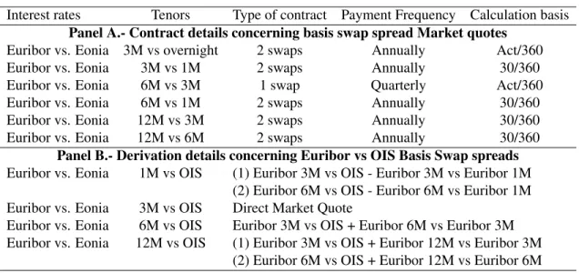
The dataset comprises weekly BS spread quotes from December 19, 2007, to Novem-ber 12, 2014, collected from BloomNovem-berg. The set of traded BS contracts is reported in Table 1, Panel A. As shown, the clauses of BS contracts are not homogeneous in several respects, such as the type of contract, the payment frequency or the basis for calculation. This heterogeneity could lead to potential bias in our results. To address this aspect, we synthetically construct homogeneous quotes through non-arbitrage for a broad spectrum
of tenors and maturities, taking the OIS rate as a reference1. To briefly illustrate our
proce-dure, consider the case of the 6-month Euribor–OIS spread, which is not directly available in the market. To construct these quotes, we combine two existing contracts: 3-month Euribor against OIS quotes and 6-month Euribor against 3-month Euribor quotes. This procedure requires the use of the BS pricing formulas provided in Appendix A of this article. A more detailed discussion could be found in Lafuente, Petit and Serrano (2015).
[TABLE 1 ABOUT HERE]
This article focuses on BS spreads of Euribor tenors against Eonia, the rate underlying the OISs. We focus on BS contracts whose payments are associated with Euro interbank
1The use of synthetic series is standard in finance research. For instance, Longstaff and Rajan (2008)
connect on-the-run series of the CDX index to obtain a virtual series of the most liquid collateral debt obligation index. In this way, many fixed-income indices are constructed using the most liquid contracts at the moment.
deposit rates with 1-, 3-, 6- and 12-month tenors. For each contract, a wide variety of maturities are considered: 1-, 3-, 5-, 7- and 10-year maturities. Table 1, Panel B dis-plays the BS spreads obtained by non-arbitrage. The evolution of the spreads over time is depicted in Figure 1. As expected, BS spreads react to financial distress and uncer-tainty. For example, Figure 1 shows that the Lehman Brothers’ bankruptcy in September 2008 resulted in a sharp rise in spreads that persisted for several weeks. Analogously, spreads rose significantly during the European sovereign debt crisis, for instance, with the Greek government bailout in May 2010 and the financial aid packages sought by Ireland in November 2010 and Spain in June 2012. Second, the term structure of BS spreads is consistently downward-sloping, especially at longer maturities (3, 6 and 12 months); this pattern is also observable at the shortest maturities during periods of stress. BS spreads also appear to respond to the non-conventional measures undertaken by the ECB during
the European sovereign crisis.2These actions anticipate a gradual decrease in BS spreads.
In sum, it appears that BS spreads reflect liquidity shortages in the financial sector and/or perceptions of higher default risk associated with lending in the interbank market.
[FIGURE 1 ABOUT HERE]
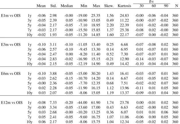
The descriptive statistics of BS increments in Table 2 provide some interesting
in-sights.3 For example, the volatilities of BS spreads are higher at short-term maturities.
This is also exacerbated at longer tenors. Moreover, note that the maximum increments in BS spreads are also concentrated in those short-term maturities, reaching 25.35 (61.90) bps in the case of a 1-month (12-month) tenor at a 1-year maturity. In addition, the dis-tribution of increments is right-skewed—particularly for shorter maturities—exhibiting a high concentration of observations at the tails. In all cases, excess kurtosis is detected, corroborating departures from normality.
2To enable banks to access funding immediately after the Lehman Brothers’ collapse, the ECB conducted
a massive injection of liquidity on October 8, 2008, and special term refinancing operations on September 29, 2008. The ECB also intervened in sovereign debt markets not only to attenuate the sharp increases in borrowing costs but also to ensure depth and liquidity in certain dysfunctional market segments. The first goal was achieved by the Securities Market Programme, introduced in May 2010, and its successor, the Outright Monetary Transactions programme, launched in August 2012. The second objective was pursued by the purchase of euro-denominated covered bonds under two programmes introduced on June 30, 2010, and October 31, 2012. Through the long-term refinancing operations (LTROs) conducted in fall 2011, the ECB also intended to enable banks to access long-term funding.
3 Standard tests for stationarity do not reject the hypothesis of the existence of a unit root of the BS
[TABLE 2 ABOUT HERE]
An inspection of the nature of market co-movements among BS quotes could also pro-vide a different perspective on the data. We conduct a principal component analysis on the entire sample of (standardised) BS spread increments. We identify the existence of strong commonality among BS spread increments, with a first principal component
ac-counting for 55.10% of the total explained variance. This percentage increases to 70.76%
and 79.33% when incorporating the information content of the second and third
compo-nents, respectively. The loadings corresponding to the first principal component are all positive and of similar magnitude, suggesting an interpretation of a level factor for this first principal component. A similar exercise for second and third components suggests
the existence of slope and curvature factors, respectively.4
According to the above results, BS spreads exhibit a downward-sloping term struc-ture. BS data also exhibit strong commonality, with the first component accounting for more than 50% of the total variance, and the term structure of BS spreads accounts for the standard level, slope and curvature factor patterns in fixed-income products. The volatil-ity at short maturities is remarkably higher than at the remaining maturities, suggesting that shocks tend to impact this section of the curve more substantially. To discuss this aspect, the next section presents a model to decompose BS spreads into their expected and unexpected drivers.
3. Model and Estimation Methodology
This section describes the empirical model used to decompose BS spreads into their expected and unexpected constituents. We also explain the econometric approach to its estimation.
3.1. MODEL SET-UP
BS contracts involve expectations of short-term interest rates at different tenors for a given maturity. Before 2008, short-term interest rates were strong predictors of their
4For the sake of robustness, we repeated this analysis by tenor. The results obtained thereby are similar in
all cases, and they are consistent with the standard interest rate term structure assessment of level, slope and curvature factor components; see, for instance, Diebold and Li (2006). To save space, complete information on the principal components structure is not reported in the tables but is available from the authors upon request.
future evolution. There were no substantial differences in the euro interbank money market in lending at compound rates of short or long tenor and, as a consequence, BS spreads were negligible. Forecastability is consistent with the idea that BS fluctuations are mainly expected; see Cochrane (1994). Thus, before 2008, the evolution of BS quotes could be described using a model of only predictable drivers.
Why should we expect an alternative evolution of BS quotes after 2008? The emer-gence of systemic, worldwide events, such as the default of Lehman Brothers or the Eu-ropean sovereign debt crisis, gives BS quotes room to react in a unexpected way. This unanticipated behaviour is consistent with the lower predictive ability of short-term inter-est rates. To reconcile these ideas, we introduce a model in which BS spreads are driven by expected shocks while allowing for the existence of unexpected regime changes. In particular, we posit the following specification for the first differences of BS spreads:
∆BSit(T) =zt+ut, (1)
where∆BSit(T)denotes the increments of the BS spread for a particular tenoriand
matu-rity (T), andzt andut denote the expected and unexpected drivers of BS spreads,
respec-tively. The unexpected componentzt is a regime-switching process:
zt+1= ( zt, with probability p gt+1, with probability 1−p ) , (2)
where processzt is a random walk with probabilityp. Otherwise, a regime change affects
its volatility, and process zt becomes gt+1, where gt+1
iid
∼N(0,σg2). The value of the zt
component remains constant over time for long periods if the probability of regime change is low.
The component ut stands for the expected shocks, and it is modelled according to a
first-order autoregressive AR(1) process with a positive autocorrelation coefficient:
ut+1=φut+et+1, with |φ |<1 (3)
The model admits an expression in state-space form as follows: " zt+1 ut+1 # = " p 0 0 φ # " zt ut # + " Nt+1 et+1 # , (4) with Nt+1= ( (1−p)zt, with probability p gt+1−pzt, with probability 1−p ) . (5)
Thus, the parameter vectorΘ of the model consists ofΘ=p,φ,σe2,σg2 , with pbeing
the probability of no regime change p, σg2the variance of the unexpected component,σe2
the variance of the expected component, andφ the AR(1) parameter associated with the
evolution of the expected shock over time. This modelling strategy has been previously employed to represent the dynamics of stochastic inflation or in the context of monetary policy to represent the dynamics of the growth rate of money supply; see, for example, Andolfatto, Hendry and Moran (2008) and Burnside, Han, Hirshleifer and Wang (2011).
3.2. ESTIMATION METHODOLOGY
This section provides the econometric procedure for estimating the parameter vector
Θ=p,φ,σe2,σg2 . Additional outputs of this procedure are the time series of
unobserv-able components ˆzt|t−1and ˆut|t−1from the BS spread data, which are also computed. Our
estimation strategy is based on the particle filter, a sequential Monte Carlo filter. This methodology overcomes the non-optimality of the Kalman filter when the vector of per-turbations in the state equation does not follow a multivariate normal distribution. In the context of our model, the state Equation (4) is a mixture of Bernoulli and Gaussian noises, which does not lead to a multivariate normal distribution.
The estimation procedure is based on the evaluation of the density function of ˆut|t−1
givenp,φ,σe2,σg2 once the signal is updated (ˆzt|t−1). Without loss of generality,z0=0.
The complete sequence is as follows:
a. For the first period, we draw a random sample of size I=1,000 from a uniform
distribution in the interval (0,1) and from a normal distribution with zero mean and
and xi1 ∼N 0,σg2, respectively, with i=1,2, ...,I. We use these two values to
generate a new sample that we denoteN1i|0as follows:
N1i|0=
(
(1−p)z0=0 if U1i ≤p
xi1−pz0=x1i if U1i >p, (6)
where(1−p) is the probability of regime change, andz0=0 by assumption. The
N1i|0values are used to generateIsamples ofzi1|0as follows:
zi1|0=pz0+N1i|0=N1i|0. (7)
b. Next, we use the first observation of the BS spreade1 and the previously estimated
values ofzi
1|0to generate a random sample of the expected component of the series
ui
1|0:
ui1|0=e1−zi1|0, withi=1,2, ...,I. (8)
c. We then evaluate the relative weight of each observationui
1|0: qui 1|0 = p(ui 1|0) I ∑ j=1 p(uj 1|0) , (9)
where the probability p(ui
1|0) corresponds to the marginal distribution of the first
observation of an AR(1) process, namely, a Gaussian distribution with zero mean and varianceσe2/(1−φ): ui1|0∼N 0,σe2/(1−φ).
d. The initial samplezi1|0is updated by performing a weighted sampling with
replace-ment in accordance with the above-replace-mentioned weights. We name these resampled valueszi1.
e. We repeat the process described above for each period, taking into account that from the second period onwards, the relative weight of each observation of the expected component will be computed according to the conditional distribution of an AR(1)
process. This means that, for a generic periodt, the conditional distribution ofuit|t−1
onui
t−1|t−2would be:
uit|t−1|uti−1|t−2∼Nφuit−1|t−2,σe2
The second step consists of computing the likelihood function of the vector of BS
spread values e≡(e1,e2, . . . ,eT)0, where T denotes its sample size. Using the Law of
Large Numbers, we compute the conditional probabilities ofet|et−1:
p(et|et−1) = 1 I I
∑
i=1 p(uit|t−1), (11) wherei=1,2, ...,I, and p(uit|t−1)is calculated according to Equation (10).
Having computed these conditional probabilities, we can evaluate the likelihood func-tion: p(e1,e2, . . . ,eT) = T
∏
t=1 " 1 I I∑
i=1 p(uti|t−1) # . (12)Finally, the likelihood function is maximised with respect top,φ,σe2,σg2 :
Max
{p,φ,σg2,σe2}
p(e1,e2, . . . ,eT). (13)
The above process can be summarised in these three basic stages. First, compute ˆ
ut|t−1, taking as given the initial values of the parametersp,φ,σe2,σg2 . Then, calculate
the likelihood function corresponding to the observable data serieset. Finally, maximise
the likelihood function with respect to model parameters.
4. Disentangling Expected from Unexpected Components of Basis Swap Spreads
4.1. PARAMETER ESTIMATES
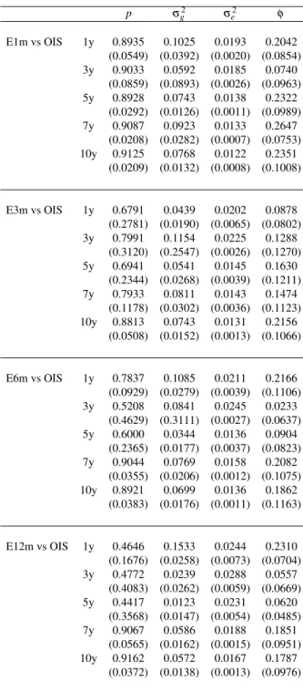
Table 4 provides the maximum likelihood estimates of the model under analysis (stan-dard deviations in parentheses). Some interesting conclusions can be drawn from this
table. First, the probability of regime change (1−p)is generally higher at shorter than
at longer maturities. For example, these probability estimates are approximately 10% for 7- and 10-year maturities, irrespective of the tenor of the contract. Notably, this differ-ence in probabilities among long-short maturities widens when increasing the tenor of the contract. See, for instance, the 1- and 12-month spreads against OIS contracts. The probability of a regime change at a 1-year maturity is approximately 11%(54%) for the 1-month (12-month) contract. These values decline to 8% when considering the 10-year
maturity for 1- and 12-month tenor contracts. These results suggest that the persistence of unexpected shocks is higher for BS spread increments at short-term maturities and longer tenors.
[TABLE 4 ABOUT HERE]
The variance estimates under regime shift σg2 differs significantly in magnitude from
σe2. Under regime shift, the variance is systematically higher than the variance under the
absence of unexpected news. These estimates depict a stressed and volatile scenario in BS spread increments when a new regime is triggered. Specifically, while unconditional
volatilities for both shocks, σg2 and σe2, are similar across tenors, for a given tenor, the
uncertainty associated with shorter maturities tends to be slightly higher. This pattern suggests that the price discovery process takes place by updating short-term expectations. This is consistent with previous results on regime-switching probabilities, suggesting that shocks prompt higher deviations in BS spread increments at these shorter maturities.
Fi-nally, note that in all cases, the autoregressive coefficientφ is statistically significant and
lower than one, reflecting that the predictability of the expected component is not remark-able.
4.2. TIME SERIES AND COMMONALITY
The time series evolution of the unexpected component, which captures regime shifts,
is displayed in Figure 2. As shown, the driver zt remains close to zero for longer
peri-ods, and it tends to suddenly change during periods of financial distress, such as after the Lehman default or the European sovereign debt crisis. Interestingly, the second Covered Bond Purchasing Programme implemented by the ECB is also noticeable in the unex-pected component. Since 2007, credit derivative markets have become more volatile, and the number and magnitude of regime changes before the implementation of this quantita-tive easing programme were much more intense than thereafter. This pattern is particularly clear for shorter tenors (1- and 3-month). Concerns revealed by derivative trading accord with the absence of a positive reaction in government yields to the foregoing bond pur-chasing programme. In-sample information suggests that BS quotes were anticipating the posterior Spanish bailout. After this event, the ECB supported bank lending and money market activity through two LTROs. This monetary intervention ultimately contributed to a sharp decline in bond yields, likely as a consequence of the carry trade, where traders
borrowed from the ECB at a 1% interest rate and then purchased higher-yield Spanish and Italian bonds. After this LTRO, the shock-driven BSs were mainly captured by the expected component.
[FIGURE 2 ABOUT HERE]
Figure 3 depicts the expected component. A visual inspection suggests that the relative importance of this component is higher than the unexpected one. For instance, we observe that expected component spreads exhibit a higher magnitude (up to 40 bps) than those originated by unexpected shocks. Moreover, the volatility of the expected component increases with tenor.
[FIGURE 3 ABOUT HERE]
A different perspective on the data is provided by the box plot in Figure 4. This figure depicts how the observations from the unexpected component are systematically located around zero; quartiles 1 to 3 are hardly distinguishable. This feature is consistent across maturities and tenors. However, the expected component observations exhibit higher dis-persion around their medians. These results reinforce the notion that the regime shifts capture the unexpected shocks that trigger greater uncertainty.
[FIGURE 4 ABOUT HERE]
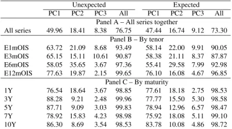
The empirical findings previously reported in Section 2 showed the existence of strong commonalities in BS spreads. As we are interested in whether the decomposed series re-produce this pattern, we perform separate principal component analyses of the expected and unexpected components. The results are provided in Table 3. From Panel A, we ob-serve that the first three principal components of the expected (unexpected) drivers account for more than 70%(75%) of the total variation. These explained variances increase when grouping the series by tenor (Panel B) and, to a greater extent, when grouping by maturity (Panel C). In the latter case, the explained variance of the three factors rises to 99%. These results show that the source of heterogeneity in expected and unexpected components is linked to the asset class and not to the maturity of the contracts, suggesting that investors might consider specific tenors for special purposes, such as liquidity. This circumstance could reflect some investors’ preferences for specific maturities, their demand for these maturities being inelastic. Along these lines, this finding could lead to an impact on BS
quotes similar to that proposed by the preferred habitat theory of sovereign bonds.5 Fi-nally, the analysis of loading coefficients for expected and unexpected components, not reported to save space, leads again to the interpretation of the first, second and third com-ponents in terms of the level, slope and curvature.
[TABLE 3 ABOUT HERE]
The empirical findings reported in the previous sections suggest two basic ideas: a) the empirical model proposed to decompose BSs into expected and unexpected drivers adequately captures stylised facts about our financial data, and b) given that strong com-monalities across tenors and maturities is observed, the behaviour of BSs should can be summarised by the first principal component.
5. Relationships between Basis Swap Components and Macroeconomic Factors
In this section, we seek to explain the fluctuations in the BS spread components with changes in the macroeconomic environment.
5.1. EXPLANATORY VARIABLES
We consider a broad set of economic and financial variables as potential explana-tory factors for BS spread components. Although countless variables could be linked to this analysis, we follow the research designs in Longstaff, Pan, Pedersen and Singleton (2011) and Groba, Lafuente and Serrano (2013) to focus on a panel of economic variables grouped into four categories: money and interest rates, stock market, credit market and risk-aversion variables. We next describe the set of variables employed.
Money and interest rate market variables. The multi-curve setting is clearly linked to
the risk of lending on the interbank market, interbank risk (Filipovic and Trolle, 2013). Therefore, interest rates attract our attention immediately. In particular, we consider the
interest rate level in the Euro Area, denotedLevel. This is the risk-free lending rate in the
Euro Area, and it is proxied by the Eonia index, which is computed as a weighted average
5The preferred habitat view proposes that investors have preferences for specific maturities and that their
demand for these maturities is somewhat inelastic, leading to an impact on interest rates; see, for instance, Greenwood and Vayanos (2010) and Greenwood and Vayanos (2014).
of all overnight actual lending transactions executed by a panel of banks in the euro money market. The Eonia index is calculated by the ECB, which is the source of these data.
Interest rate slopes (Slope) are also taken as usual indicators of overall economic
health; see Collin-Dufresne, Goldstein and Martin (2001) and Groba, Diaz and Serrano (2013). The risk-free interest rate slope in the Euro Area is proxied by the spread between the 10-year and 2-year Eonia swap quotes. Eonia swaps, or OIS, are similar to vanilla IRS transactions—they both are exchanges of fixed and variable interest rates—with the variable rate being linked to the Eonia Index. These data were obtained from Bloomberg.
In addition to these variables, information on liquidity in the money market is consid-ered in our analysis through the ECB Liquidity Indicator for the Euro Area money market
(Liquidity) published by the ECB. This composite indicator includes arithmetic averages
of individual liquidity measures. These variables were drawn from the ECB, the Bank of England, Bloomberg, JPMorgan Chase & Co. and Moody’s KMV.
Stock market variables. This group includes the Euro Stoxx Banks Price index, a
capitalisation-weighted index that reflects the stock performance of companies in the Eu-ropean Monetary Union (EMU) that are involved in the banking sector. Additionally, we
exploit information from the Euro Stoxx VIX (EuroVix) index on market sentiment
re-garding future volatility. This index is based on a weighted average of implied volatilities of options written on EuroStoxx 50 stocks. It captures the implied volatility on Eurex-traded options with a rolling 30-day expiry. All of these variables were collected from Bloomberg.
Credit market variables. This group of variables includes the Itraxx Senior Financials,
an index that comprises 25 equally weighted CDSs on investment-grade European finan-cial sector entities. The maturity of CDS contracts is 5 years. This index is a proxy for the
aggregate default risk in the financial sector, and it is denotedCDS Financials. The data
were obtained from Markit. Additionally, we incorporate the Federal Republic of
Ger-many Senior CDS quotes (CDS Germany) with a 5-year maturity. The German sovereign
CDSs provide information on sovereign risk linked to the risk-free asset–German bunds are usually considered risk-free assets in the Euro Area context. These spreads are in USD and have been drawn from Bloomberg. We also incorporate the spread between the 1-year maturity AAA EUR Financial Sector and the 1-1-year maturity German Government
yields (FinGvt) into our study. This spread captures the tensions between the financial and
com-ponent of the CDS portfolio of European banks in Rodríguez-Moreno and Pena (2013),
and it could be employed as a proxy for systemic risk.6 These yields are calculated as a
composite yield of representative securities around the 1-year maturity. This variable is also provided by Bloomberg. To complete the set of credit variables, we include the ECB
Systemic Stress Composite Indicator Index (SSCI index), an indicator of contemporaneous
stress in the financial system suggested by Holló, Kremer and Duca (2012) and provided by the ECB.
Risk-aversion variables. Regarding the market appetite for risk, we include the ECB
Risk Aversion Indicator, denotedRisk aversion. This indicator is constructed as the first
principal component of five risk-aversion indicators, namely, Commerzbank Global Risk Perception, UBS FX Risk Index, Westpac Risk Appetite Index, BoA ML Risk Aversion Indicator and Credit Suisse Risk Appetite Index. Higher values of this indicator denote an increase in market-wide risk aversion. This indicator comes from Bloomberg, Bank of America Merrill Lynch, UBS, Commerzbank and ECB calculations.
Standard stationarity tests do not reject the existence of unit roots at usual confidence intervals for the explanatory variables in levels. When taking first differences, stationarity is not rejected. Thus, we consider the set of regressors in first differences. To prevent the use of variables with similar information content, a correlation matrix for our explana-tory variables is computed. In statistics not provided here but available upon request, we observe that the EuroStoxx Banks index and EuroStoxx VIX are highly correlated with the Itraxx Financial and ECB risk-aversion indexes. Further, the Itraxx Financial index exhibits a strong correlation with German CDS spreads. To avoid multicollinearity prob-lems, we remove the stock market variables and the Itraxx Senior Financial index from our study.
5.2. OLS REGRESSIONS
To analyse the relationships of BS components with macroeconomic and financial sources of risk, we estimate a set of OLS regressions. In particular, we initially project the first and second principal components of the expected and unexpected drivers onto our
set of explanatory variables. Let ∆PCi jt denote the increments of principal component
i for expected and unexpected component j at time t. Then, we consider the following
specification for each component:
∆PCi jt =αi j + β1,i j∆Levelt+β2,i j ∆Slopet+β3,i j ∆Liquidityt
+ β4,i j∆CDS Germanyt+β5,i j∆FinGvtt+β6,i j ∆Risk aversiont
+ β7,i j∆SSCI Indext+εi jt, i=1,2, j=1,2. (14)
whereθi j
αi j,βi j0
0
withβi j= (β1,i j, ...,β6,i j)denotes the vector of unknown parameters,
andεi jt is a disturbance assumed to obey standard assumptions.
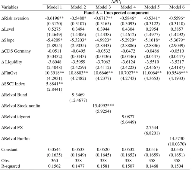
To sequentially observe the importance of each exogenous variable, Table 5 reports the estimated slopes for nested specifications. This table reports the estimated parameters,
White (1980) robust standard errors and adjustedR2coefficients for unexpected (Panel A)
and expected (Panel B) components of BS spreads. Some brief comments follow. The most interesting result in Panel A is the correlation between the first principal component of unexpected spreads and the spread between financial and (risk-free) sovereign debt. The coefficient is positive and statistically significant at the 1% confidence level. Moreover,
the R-squared coefficient jumps from 8.49% to 14.62% when this variable is included.
This result is economically relevant, as it connects the overall financial system with the unexpected component of BS: increased financial tensions are related to increments in this first component, a cross-sectional average of BS spreads at different maturities. In this way, we consider a possible link between BS and risk in the financial system, or systemic risk. The recent paper of Ramsay and Sarlin (2015) shows that the relationship between the stock of total debt and the growth in the gross savings of nations is an indicator of systemic risk and vulnerability. Therefore, debt sustainability concerns in peripheral countries after the Greek sovereign default may partially explain the importance of default risk. More recently, Delatte, Fouquau and Portes (2017) also find evidences of bank credit risk as a driver of regime switches in long-term sovereign spreads.
[TABLE 5 ABOUT HERE]
The second principal component concerning the unexpected component is related to
market-wide liquidity. The increments of liquidity explain a non-negligible 10.97%. The
coefficient associated with liquidity is negative and statistically significant at the 5% con-fidence level. This variable remains significant after incorporating our proxy for systemic
risk as an additional explanatory variable. The negative sign of the coefficient suggests that a reduction in market-wide liquidity is related to increases in financing costs.
Regarding the expected component, the OLS estimates in Table 5 (Panel B) highlight the importance of risk aversion, irrespective of the model under consideration. Agents’ perceptions of market uncertainty are clearly reflected in the expected component of BS quotes. Analogously to risk aversion, our proxy for sovereign risk (5-year German CDS)
is statistically significant at conventional levels. TheR2coefficient increases from 7.19%
(Model 1) to 10.83% (Model 4) when sovereign risk is included. The slope of the interest
rates emerges as a statistically significant determinant of additional commonality. The
second principal component, which captures a remarkable 26.48% of the total variability,
is significant and positively covaries with the slope, which contains information about business cycle and monetary policy shocks.
The previous findings support our empirical decomposition of interbank risk into these underlying drivers. Unexpected components in BS spreads are related primarily to the arrival of financial systemic and liquidity shocks. However, expected components are related to the time-varying evolution of risk aversion and overall economic health proxies, such as the interest rate slope and risk-free sovereign spread.
5.3. IMPULSE RESPONSE FUNCTIONS
Next, we complete the empirical presentation at Section 5 by reporting the impulse re-sponse functions of the principal components previously extracted from the expected and unexpected components of BSs. We estimate four VARs. The variables included are se-lected according to the variables that emerge as significant in the OLS regressions. A first VAR includes the first principal component that emerges from the unexpected drivers, as well as the 1-year maturity AAA EUR Financial Sector spread, risk aversion and systemic risk. A second VAR is based on the second principal component from unexpected drivers, and the liquidity variable.
Concerning the expected components, a third VAR is estimated including the first com-ponent of expected drivers, risk aversion and German CDS. Finally, a fourth VAR includes the second principal component from expected drivers of BSs, risk aversion and the slope of the interest rates.
The structural identification we use is based on a Cholesky decomposition of the variance-covariance matrix. The causal ordering is in accordance with the sequence in
the foregoing explanation for each VAR7. The lag length was determined using the Akaike information criterion. In all cases, the optimal number of lags is two.
Figure 5 reveals some interesting aspects for the unexpected component. The re-sponses in first principal component to shocks in our proxies of systemic risk and risk aversion spread are positive and statistically significant. As expected, when systemic risk or risk aversion increase, financing costs tend to be higher. In both cases, the effect of a shock vanishes in the short-term, after a couple of weeks. However, the impact of a shock in the stress variable is not statistically significant at any time. While point responses to the
stress variableSSCindexare positive over time, the lack of precision leads us to conclude
that the responses are not statistically significant at the 5% level. With regard to a liquidity shock in the second component of unexpected BS spreads, this impulse is associated with a negative responses, and the transmission persists for an extended period of time, namely, six weeks. When the ability of banks to fund their positions and/or the ability to trade improves, financing costs tend to be lower during the next six weeks.
[FIGURE 5 ABOUT HERE]
The responses of the principal components obtained with the expected constituents of BSs are depicted in Figure 6. All of the responses reproduce an overshooting path, be-ing only significant to shocks from the slope of the term structure of interest rates and risk aversion. The response of the expected component in reaction to the slope just vanishes af-ter one week. When investors obtain additional compensation for longer maturity bonds, the preference of financial intermediaries towards short-term maturities temporarily de-creases. On the contrary, an increase in risk aversion initially intensifies the short-term bias. The reaction for the second week becomes negative, probably reflecting the updating of the risk-return relationship across the maturity spectrum. After three weeks, shock is wholly accommodated by the market.
[FIGURE 6 ABOUT HERE]
7Assuming that principal components are affected by structural shocks for remaining variables involved,
6. Robustness Checks
This section examines the robustness of our results to different specifications of the model. In Section 6.1, we discuss the OLS estimates with alternative proxies of systemic risk. In Section 6.2, we test whether volatility, rather than systemic risk, is the source of covariance in our estimations. Finally, we conduct additional analyses using alternative liquidity controls from money markets in Section 6.3. The main conclusion of all of these analyses is that the results are robust to the alternatives discussed.
6.1. SYSTEMIC RISK VARIABLES
The concept of systemic risk involves several aspects, such as triggering events, fi-nancial contagion, chain reactions and global disruption. Recent papers (see, for instance, Adrian and Brunnermeier (2016), López-Espinosa, Moreno, Rubia and Valderrama (2015) and Rodríguez-Moreno and Pena (2013)) have addressed the relevance of the measure to be considered. Among a wide variety of alternatives, the CoVaR measure of Adrian and Brunnermeier (2016) has been adopted as an international standard. This measure is de-fined as the difference between the conditional value at risk of the financial system, condi-tional on an institution being in distress, and the CoVaR condicondi-tional on the median state of the institution (Adrian and Brunnermeier, 2016). Along these lines, we employ the CoVaR
series for the European banking (CoVaR banks) and insurance (CoVaR insurance) sectors
at different percentiles, as provided by the ECB. Additionally, we consider a composite
indicator of systemic risk from cross-subindex correlations (Crossub Index) in Holló et al.
(2012), also provided by the ECB.
Table 6 reports the projections of the first principal component extracted from the unexpected drivers of BSs for the different proxies for systemic risk. Only the measure based on cross-subindex correlations is not statistically significant at standard confidence levels.
Regarding the remaining alternative proxies, the 1-year maturity AAA EUR Finan-cial Sector spread appears to be a substitute for the CoVaR measure. When the spread is excluded, the CoVar variables become significant. However, when all of the proxies are included, the spread appears to capture all of the information content in the CoVar mea-sures. Our initial systemic risk variable is significant, but none of the CoVar variables are relevant. As expected, the point estimates for all of the CoVar measures are negative,
in-dicating that an increase in financing costs tends to reduce the CoVar measure, worsening the conditional VaR of a given financial institution with respect to the financial system.
However, the ECB composite indicator of systemic risk captures complementary
in-formation, remaining significant in presence of theSSCI Index spread. We conclude that
systemic risk plays a significant role in explaining unexpected changes in BSs. [TABLE 6 ABOUT HERE]
6.2. VOLATILITY VARIABLES
To address the possibility that financial stress could be due to volatility instead of sys-temic risk, we select different measures of realised volatility from different assets: German
bonds (Relvol Bund), non-financial stocks (Stock nonfin), foreign exchange rates (Relvol
FX) and 3-month Euribor rates (Relvol Eur3m). We repeat our regression exercises
indi-vidually including the realised volatility variables, and the results are provided in Table 7. The explanatory power of the model remains similar in all cases, and statistical signif-icance is obtained only for the realised volatility of the non-financial stocks. Our findings confirm the role played by systemic risk.
[TABLE 7 ABOUT HERE]
6.3. ADDITIONAL ANALYSES
Finally, we conduct additional analyses using alternative liquidity controls from money
markets. We select a set of liquidity variables: main refinancing operations (MRO),
long-term refinancing operations (LTRO), margin lending facility (Margin lending facility),
level of current accounts (Current accounts) and deposit facilities (Deposit facility) in
the ECB.
Table 8 reports the OLS estimates of the second principal component concerning the unexpected constituent of BS spreads. None of the controls used are statistically significant at standard levels, corroborating that liquidity is adequately accounted for by the proxy variable supplied by the ECB.
7. Conclusions
Money markets have experienced important changes since 2008. Market participants have begun to work with multi-curve interest rates. In this new framework, BS spreads are clear candidates for revealing information about how market participants respond to credit risk.
In this paper, we propose an empirical decomposition of BSs into expected and unex-pected constituents. Exunex-pected shocks account for the continuous arrival of information to the market, and unexpected shocks represent uncommon information reaching the market. The main objective is to analyse the nature of the effects of credit and liquidity risk while also accounting for the role of systemic risk. We provide a deep characterisation of the different impacts of shocks and their relative importance across tenors and maturities.
Our findings show that after 2008, credit derivative markets clearly incorporate the instability of the European financial system. For short tenors, both credit and liquidity risks are associated with unexpected drivers. Liquidity shocks tend to affect short maturities, while credit shocks are associated with medium- to long-term maturities. For long tenors, interbank credit risk becomes expected while liquidity risk remains unexpected, although its effect is on the entire term structure.
Our interpretation of the results is that although interbank credit risk is the predomi-nant and most common source of fluctuations affecting the entire term structure, as tenors increase, their impact becomes more expected, meaning that credit shocks are of shorter duration. Liquidity shocks are unexpected, which means that their impact is long lasting, although these shocks are less frequent. For shorter tenors, liquidity shocks only matter at shorter maturities, but importantly, for longer tenors, they have an impact on the entire term structure.
Systemic risk also plays a significant role in explaining the changing nature of uncer-tainty in the interbank credit market. A potential European breakdown is now being priced in the market. The vulnerability of peripheral countries due to excessive leverage could be part of the problem. However, institutional factors, such as the lack of fiscal integration in the European Union, represent avenues for additional research.
Appendix A. The Basis Swap Contract
There exist two types of single-currency BS contracts exchanged in the interbank mar-ket. First, there are the BSs constituted by two vanilla swaps—here, the first type. Second, we have single line items—the second type—which consist of the interchange of two float-ing rates, the longer tenor Euribor rate against the shorter tenor rate plus a spread. In any case, there are negligible differences between the quotes of the two types of swaps, mainly due to the frequency of compounding and the day count conventions, as we will see in more detail below. This paper employs the first type of BS contract, which are quoted as a portfolio of two standard floating versus fixed swaps with two different floating rates and coincident fixed leg tenors. In this case, the BS spread is the difference between the two equilibrium fix-to-float swap rates, and it has the same payment frequency as the shorter fixed leg tenor in the swap. Then, the value of the BS contract is:
∆x,y = IRS(t;Tx,Tz)−IRS(t;Ty,Tz) = Et ∑nj=x1e− RTx,j t r(s)dsτ x Tx,j−1,Tx,j L Tx,j−1,Tx,j −Et ∑njy=1e− RTy,j t r(s)dsτ y Ty,j−1,Ty,j L Ty,j−1,Ty,j ∑njy=1Pd t,Tz,j τz Tz,j−1,Tz,j , (15)
withIRS(t;Tx,Tz)andIRS(t;Ty,Tz)being the equilibrium swap rates of fixed versus float-ing IRS contracts, and the floatfloat-ing legs are linked to the x-tenor and y-tenor Euribor refer-ence rates, respectively.
In the second type of basis swap contract, the longer tenor Euribor rateL(Tx,j−1,Tx,j)
is exchanged for the shorter tenor Euribor rate L(Ty,j−1,Ty,j). The date schedules
corre-sponding to the swap floating legs linked to Euribor ratesL(Ty,j−1,Ty,j)andL(Tx,j−1,Tx,j)
areTy={Ty,0, ..,Ty,ny}andTx={Tx,0, ..,Tx,nx}, respectively. To balance the present value
of these legs, a BS spread∆x,yhas to be added to the floating leg with shorter tenor. The
second type is structured as a floating vs. floating swap plus spread. In this case, the BS spread has the same payment frequency as the shorter tenor leg and is quoted against
this leg. In the second type of BS contract, the longer tenor Euribor rate L(Tx,j−1,Tx,j)
is exchanged for the shorter tenor Euribor rate L(Ty,j−1,Ty,j). The date schedules
areTy={Ty,0, ..,Ty,ny}andTx={Tx,0, ..,Tx,nx}, respectively. To balance the present value
of these legs, a BS spread∆x,yhas to be added to the floating leg with shorter tenor. The
value of the BS contract is as follows:
BasisSwap(t;Tx,Ty) = Et nx
∑
j=1 e− RTx,j t r(s)dsτ x Tx,j−1,Tx,j L Tx,j−1,Tx,j ! − Et ny∑
j=1 e− RTy,j t r(s)dsτ y Ty,j−1,Ty,j L Ty,j−1,Ty,j +∆x,y ! . (16) This equilibrium BS satisfies:∆x,y = Et ∑nj=x1e− RTx,j t r(s)dsτ x Tx,j−1,Tx,j L Tx,j−1,Tx,j −Et ∑njy=1e− RTy,j t r(s)dsτ y Ty,j−1,Ty,j L Ty,j−1,Ty,j ∑nj=y1Pd t,Ty,jτy Ty,j−1,Ty,j . (17)
As can be observed from the previous equations, the difference between the two types of BSs is in the annuity term in the denominator, where the frequency and calculation basis in one case corresponds to the shorter tenor floating leg and in the other case to the swap
fixed leg. In particular, the first type of contract basis spread∆1x,ycan be deduced from that
corresponding to the second type of BS contract∆2x,yas follows:
∆2x,y= ∑nj=z 1Pd t,Tz,j τz Tz,j−1,Tz,j ∑njy=1Pd t,Ty,j τy Ty,j−1,Ty,j ∆ 1 x,y. (18)
References
Adrian, T. and Brunnermeier, M. K. (2016), ‘Covar’, American Economic Review
7(106), 1705–1741.
Andolfatto, D., Hendry, S. and Moran, K. (2008), ‘Are inflation expectations rational?’,
Journal of Monetary Economics55(2), 406–422.
Angelini, P., Nobili, A. and Picillo, M. C. (2011), ‘The interbank market after august 2007:
what has changed and why?’,Journal of Money, Credit and Banking43(5), 923–958.
Beirne, J. (2012), ‘The eonia spread before and during the crisis of 2007-2009: the role of
liquidity and credit risk’,Journal of International Money and Finance31, 534–551.
Burnside, C., Han, B., Hirshleifer, D. and Wang, T. Y. (2011), ‘Investor Overconfidence
and the Forward Premium Puzzle’,Review of Economic Studies78, 523–558.
Cochrane, J. H. (1994), ‘Permanent and transitory components of gnp and stock prices’,
The Quarterly Journal of Economics109(1), 241–265.
Collin-Dufresne, P., Goldstein, R. S. and Martin, J. S. (2001), ‘The determinants of credit
spread changes’,The Journal of Finance56(6), 2177–2207.
Delatte, A.-L., Fouquau, J. and Portes, R. (2017), ‘Regime-dependent sovereign risk
pric-ing durpric-ing the euro crisis’,Review of Finance21(1), 363–385.
Diebold, F. X. and Li, C. (2006), ‘Forecasting the term structure of government bond
yields’,Journal of Econometrics130(2), 337–364.
Eisenschmidt, J. and Tapking, J. (2009), Liquidity risk premia in unsecured interbank money markets. ECB Working Paper.
Filipovic, D. and Trolle, A. B. (2013), ‘The term structure of interbank risk’, Journal of
Financial Economics109(4), 707–733.
Greenwood, R. and Vayanos, D. (2010), ‘Price pressure in the government bond market’,
American Economic Review100(2), 585–590.
Greenwood, R. and Vayanos, D. (2014), ‘Bond supply and excess bond returns’,Review
Groba, J., Diaz, A. and Serrano, P. (2013), ‘What drives corporate default risk premia?
evidence from the cds market’,Journal of International Money and Finance(37), 529–
563.
Groba, J., Lafuente, J. A. and Serrano, P. (2013), ‘The impact of distressed economies on
the EU sovereign market’,Journal of Banking & Finance37(7), 2520–2532.
Henrard, M. (2014), Interest rate modelling in the multi-curve framework, 1st edn,
Pal-grave Macmillan.
Holló, D., Kremer, M. and Duca, M. L. (2012), ‘CISS - A composite indicator of systemic stress in the financial system’. ECB Working Paper Series, No. 1426.
Hu, G. X., Pan, J. and Wang, J. (2013), ‘Noise as information for illiquidity’,Journal of
Finance68(6), 2341–2382.
Lafuente, J., Petit, N. and Serrano, P. (2015), Determinants of the multiple-term
struc-tures from interbank rates. UC3M Working Papers Business, available at
http://e-archivo.uc3m.es/handle/10016/21163.
Longstaff, F. A., Pan, J., Pedersen, L. H. and Singleton, K. J. (2011), ‘How sovereign is
sovereign credit risk?’,American Economic Journal: Macroeconomics3(2), 75–103.
Longstaff, F. A. and Rajan, A. (2008), ‘An empirical analysis of the pricing of
collateral-ized debt obligations’,The Journal of Finance63(2), 529–563.
López-Espinosa, G., Moreno, A., Rubia, A. and Valderrama, L. (2015), ‘Systemic risk
and asymmetric responses in the financial industry’, Journal of Banking and Finance
58, 471–485.
McAndrews, J., Sarkar, A. and Wang, Z. (2017), ‘The effect of the term auction facility on
the london inter-bank offered rate’,Journal of Banking & Finance. forthcoming.
Mercurio, F. (2009), Interest rates and the credit crunch: new formulas and market models. Technical report, QFR, Bloomberg, 7, 22, 24.
Michaud, F.-L. and Upper, C. (2008), ‘What drives interbank rates? evidence from the
Pan, J. U. N. and Singleton, K. J. (2008), ‘Default and recovery implicit in the term
struc-ture of sovereign CDS spreads’,The Journal of Finance63(5), 2345–2384.
Ramsay, B. A. and Sarlin, P. (2015), ‘Ending over-lending: assessing systemic risk with debt to cash flow’. ECB Working Paper Series, No. 1769.
Rodríguez-Moreno, M. and Pena, J. I. (2013), ‘Systemic risk measures: the simpler the
better?’,Journal of Banking and Finance37, 1817–1831.
Rubia, A., Sanchis-Marco, L. and Serrano, P. (2016), ‘Market illiquidity and pricing
er-rors in the term structure of CDS spreads’,Journal of International Money & Finance
pp. 223–252.
Schwartz, K. (2010), Mind the gap: disentangling credit and liquidity in risk spreads. Working Paper, The Wharton School, University of Pennsylvania.
White, H. (1980), ‘A heteroskedasticity-consistent covariance matrix estimator and a direct
Table 1: Contract details concerning basis swap spread market quotes
Interest rates Tenors Type of contract Payment Frequency Calculation basis
Panel A.- Contract details concerning basis swap spread Market quotes
Euribor vs. Eonia 3M vs overnight 2 swaps Annually Act/360
Euribor vs. Eonia 3M vs 1M 2 swaps Annually 30/360
Euribor vs. Eonia 6M vs 3M 1 swap Quarterly Act/360
Euribor vs. Eonia 6M vs 1M 2 swaps Annually 30/360
Euribor vs. Eonia 12M vs 3M 2 swaps Annually 30/360 Euribor vs. Eonia 12M vs 6M 2 swaps Annually 30/360
Panel B.- Derivation details concerning Euribor vs OIS Basis Swap spreads
Euribor vs. Eonia 1M vs OIS (1) Euribor 3M vs OIS - Euribor 3M vs Euribor 1M (2) Euribor 6M vs OIS - Euribor 6M vs Euribor 1M Euribor vs. Eonia 3M vs OIS Direct Market Quote
Euribor vs. Eonia 6M vs OIS Euribor 3M vs OIS + Euribor 6M vs Euribor 3M Euribor vs. Eonia 12M vs OIS (1) Euribor 3M vs OIS + Euribor 12M vs Euribor 3M
Table 2: Summary statistics of basis swap increments
ρN
Mean Std. Median Min Max Skew. Kurtosis 30 60 90 N
E1m vs OIS 1y -0.06 2.98 -0.00 -19.00 25.35 1.56 24.83 -0.00 -0.06 -0.04 360 3y -0.05 2.39 0.05 -10.90 15.05 0.49 11.22 -0.00 -0.07 -0.02 360 5y -0.04 2.17 -0.05 -7.10 18.95 2.20 22.39 0.01 -0.02 -0.00 360 7y -0.03 2.17 -0.00 -15.50 15.85 1.37 25.38 -0.08 0.02 -0.00 360 10y -0.02 1.93 -0.05 -11.20 14.85 1.60 22.17 -0.07 0.00 -0.02 360 E3m vs OIS 1y -0.10 3.11 -0.10 -11.05 13.40 0.25 6.68 -0.07 -0.08 0.02 360 3y -0.06 2.57 -0.10 -9.45 13.30 0.14 6.95 0.01 -0.07 0.01 360 5y -0.04 2.47 0.00 -8.20 11.40 0.52 7.30 -0.07 -0.07 0.01 360 7y -0.04 2.83 -0.02 -16.90 15.15 -0.21 12.90 -0.14 -0.03 -0.07 360 10y -0.04 2.15 -0.05 -12.19 14.90 0.49 14.42 -0.10 -0.04 -0.04 360 E6m vs OIS 1y -0.10 3.88 -0.05 -15.00 30.20 1.43 16.41 -0.03 -0.07 0.01 360 3y -0.03 2.62 -0.15 -10.70 14.20 0.14 6.67 -0.01 -0.05 0.02 360 5y -0.00 2.36 -0.05 -7.70 12.35 0.68 7.51 -0.02 -0.02 0.07 360 7y 0.02 2.28 -0.05 -11.90 16.15 1.12 13.96 -0.11 0.01 0.05 360 10y 0.03 2.07 -0.05 -8.06 15.05 1.19 13.37 -0.09 -0.03 0.04 360 E12m vs OIS 1y -0.08 7.33 -0.20 -44.00 61.90 1.74 23.78 0.00 -0.01 0.02 360 3y -0.00 3.34 -0.05 -13.60 17.00 0.43 6.63 -0.02 -0.00 0.02 360 5y 0.03 2.68 -0.00 -10.20 13.25 0.36 6.07 0.01 0.01 0.06 360 7y 0.05 2.41 -0.05 -9.60 16.75 1.07 11.06 -0.06 0.00 0.05 360 10y 0.06 2.17 0.05 -8.06 15.75 1.04 12.34 -0.05 -0.02 0.02 360
Descriptive statistics for increments of BS spreads. BS contracts are Euribor against Eonia at different tenors and maturities. Euribor has 1-, 3-, 6- and 12-month tenors. The contracts have 1-, 3-, 5-, 7- and 10-year maturities. The table presents means, standard deviations, medians, minimums, maximums, skewness, kurtosis and 30, 60 and 90 autocorrelation lags. Increments are expressed in basis points and correspond to weekly data from December 19, 2007, to November 12, 2014.
Table 3: Explained variance of unexpected and expected principal components
Unexpected Expected
PC1 PC2 PC3 All PC1 PC2 PC3 All
Panel A – All series together
All series 49.96 18.41 8.38 76.75 47.44 16.74 9.12 73.30 Panel B – By tenor E1mOIS 63.72 21.09 8.68 93.49 58.14 22.00 9.91 90.05 E3mOIS 65.15 15.11 10.61 90.87 58.38 21.11 8.37 87.87 E6mOIS 58.05 35.65 3.67 97.36 55.41 29.58 7.99 92.98 E12mOIS 77.63 19.87 2.15 99.65 76.10 16.08 4.67 96.85 Panel C – By maturity 1Y 76.54 18.64 3.67 98.85 77.61 18.18 2.75 98.53 3Y 88.28 9.21 2.48 99.96 77.77 15.50 5.30 98.58 5Y 87.71 9.09 3.03 99.83 78.94 12.96 6.57 98.47 7Y 78.92 15.83 4.23 98.98 75.92 18.08 5.11 99.10 10Y 86.30 8.69 3.54 98.53 83.78 10.08 4.86 98.72
Principal component analysis (PCA) results for the BS tenors’ unexpected and expected factors grouped according to the maturity of the BS spreads. The table presents the percentage variance of the different BS maturities’ unexpected and expected factors explained by their first principal components. These figures are computed by performing a PCA separately for the unexpected and expected factors associated with the maturities of the different tenors’ BS spreads. The Euribor tenors are 1, 3, 6 and 12 months. The historical series of the factors correspond to weekly data from December 19, 2007, to November 12, 2014.
Table 4: Model Estimation Results p σg2 σe2 φ E1m vs OIS 1y 0.8935 0.1025 0.0193 0.2042 (0.0549) (0.0392) (0.0020) (0.0854) 3y 0.9033 0.0592 0.0185 0.0740 (0.0859) (0.0893) (0.0026) (0.0963) 5y 0.8928 0.0743 0.0138 0.2322 (0.0292) (0.0126) (0.0011) (0.0989) 7y 0.9087 0.0923 0.0133 0.2647 (0.0208) (0.0282) (0.0007) (0.0753) 10y 0.9125 0.0768 0.0122 0.2351 (0.0209) (0.0132) (0.0008) (0.1008) E3m vs OIS 1y 0.6791 0.0439 0.0202 0.0878 (0.2781) (0.0190) (0.0065) (0.0802) 3y 0.7991 0.1154 0.0225 0.1288 (0.3120) (0.2547) (0.0026) (0.1270) 5y 0.6941 0.0541 0.0145 0.1630 (0.2344) (0.0268) (0.0039) (0.1211) 7y 0.7933 0.0811 0.0143 0.1474 (0.1178) (0.0302) (0.0036) (0.1123) 10y 0.8813 0.0743 0.0131 0.2156 (0.0508) (0.0152) (0.0013) (0.1066) E6m vs OIS 1y 0.7837 0.1085 0.0211 0.2166 (0.0929) (0.0279) (0.0039) (0.1106) 3y 0.5208 0.0841 0.0245 0.0233 (0.4629) (0.3111) (0.0027) (0.0637) 5y 0.6000 0.0344 0.0136 0.0904 (0.2365) (0.0177) (0.0037) (0.0823) 7y 0.9044 0.0769 0.0158 0.2082 (0.0355) (0.0206) (0.0012) (0.1075) 10y 0.8921 0.0699 0.0136 0.1862 (0.0383) (0.0176) (0.0011) (0.1163) E12m vs OIS 1y 0.4646 0.1533 0.0244 0.2310 (0.1676) (0.0258) (0.0073) (0.0704) 3y 0.4772 0.0239 0.0288 0.0557 (0.4083) (0.0262) (0.0059) (0.0669) 5y 0.4417 0.0123 0.0231 0.0620 (0.3568) (0.0147) (0.0054) (0.0485) 7y 0.9067 0.0586 0.0188 0.1851 (0.0565) (0.0162) (0.0015) (0.0951) 10y 0.9162 0.0572 0.0167 0.1787 (0.0372) (0.0138) (0.0013) (0.0976)
Maximum likelihood estimation results using the particle filter. The table reports the maximum likelihood estimation results corresponding to the model parameters. These estimations have been calculated for the 1-, 3-1-, 6- and 12-month BS tenors and the 1-1-, 3-1-, 5-1-, 7- and 10-year maturities. The sample period considered in these estimations corresponds to basis swap spread weekly data from December 19, 2007, to November 12, 2014.
T able 5: Nested OLS rob ust re gressions of principal components ∆ P C1 ∆ P C2 V ariables Model 1 Model 2 Model 3 Model 4 Model 5 Model 6 Model 7 Model 1 Model 2 Model 3 Model 4 Model 5 Model 6 Model 7 P anel A – Unexpected component ∆ Risk av ersion -0.3392 -0.3369 -0.2983 -0.3165 -0.4027 -0.5115* -0.6196** 0.0063 0.0236 0.0282 -0.0288 -0.0911 -0.0961 -0.1087 (0.2935) (0.2937) (0.2690) (0.2905) (0.3059) (0.2987) (0.3120) (0.1991) (0.2053) (0.1896) (0.1704) (0.1316) (0.1369) (0.1477) ∆ Le v el -0.1046 -0.0720 -0.0836 1.1795 0.2228 0.5275 -0.7808 -0.7770 -0.8130 0.0994 0.0548 0.0903 (1.0672) (1.0572) (1.0708) (1.3197) (1.4418) (1.4649) (1.5804) (1.5878) (1.5946) (1.3255) (1.2929) (1.3295) ∆ Slope -3.0506 -3.0244 -4.2119 -5.1567* -5.4209* -0.3631 -0.2816 -1.1394 -1.1834 -1.2141 (2.9001) (2.8955) (3.0571) (2.8824) (2.8955) (2.1497) (2.1597) (1.7919) (1.7955) (1.8110) ∆ CDS German y 0.0072 -0.0191 -0.0488 -0.0511 0.0225 0.0035 0.0021 0.0019 (0.0440) (0.0447) (0.0448) (0.0432) (0.0233) (0.0235) (0.0240) (0.0240) ∆ Liquidity -5.3726** -3.5026 -3.6048 -3.8808** -3.7937* -3.8056* (2.5660) (2.4289) (2.4048) (1.5550) (1.9428) (1.9557) ∆ FinGvt 11.1844*** 10.3918** 0.5208 0.4286 (4.2080) (4.2931) (3.4779) (3.5386) ∆ SSCI Inde x 5.8841** 0.6849 (2.8441) (1.7473) Constant -0.0031 -0.0042 0.0004 -0.0001 0.0587 0.0479 0.0544 0.0001 -0.0082 -0.0077 -0.0094 0.0331 0.0326 0.0333 (0.1664) (0.1657) (0.1645) (0.1639) (0.1707) (0.1637) (0.1635) (0.1018) (0.0955) (0.0940) (0.0936) (0.0932) (0.0943) (0.0946) Obs. 360 360 360 360 360 360 360 360 360 360 360 360 360 360 R-squared 0.0062 0.0062 0.0121 0.0122 0.0849 0.1462 0.1562 0.0000 0.0036 0.0039 0.0061 0.1090 0.1093 0.1097 P anel B – Expected component ∆ Risk av ersion 1.1254*** 1.0715*** 1.0706*** 0.7761*** 0.7963*** 0.7432*** 0.7613*** 0.8737*** 0.8435*** 0.7557*** 0.6728*** 0.6552*** 0.6153*** 0.6125*** (0.2490) (0.2507) (0.2408) (0.2830) (0.2888) (0.2811) (0.2921) (0.1591) (0.1621) (0.1299) (0.1433) (0.1464) (0.1486) (0.1594) ∆ Le v el 2.4281* 2.4273* 2.2413 1.9448 1.4776 1.4267 1.3640 1.2900 1.2376 1.4952 1.1444 1.1523 (1.3855) (1.3976) (1.3932) (1.4741) (1.4664) (1.4766) (1.3880) (1.3875) (1.3936) (1.3393) (1.1393) (1.1643) ∆ Slope 0.0736 0.4940 0.7728 0.3114 0.3556 6.9372*** 7.0556*** 6.8134*** 6.4670*** 6.4602*** (3.2387) (3.2097) (3.2858) (3.2435) (3.2657) (1.4153) (1.4089) (1.4786) (1.4891) (1.5074) ∆ CDS German y 0.1160** 0.1222*** 0.1076** 0.1080** 0.0327* 0.0273 0.0164 0.0163 (0.0450) (0.0468) (0.0493) (0.0494) (0.0168) (0.0174) (0.0182) (0.0181) ∆ Liquidity 1.2613 2.1744 2.1915 -1.0957 -0.4101 -0.4128 (2.2990) (2.3356) (2.3361) (1.2017) (1.4672) (1.4690) ∆ FinGvt 5.4612 5.5937 4.1005 4.0800 (4.8608) (4.7582) (2.7846) (2.7777) ∆ SSCI Inde x -0.9837 0.1525 (3.0091) (1.5626) Constant 0.0101 0.0359 0.0358 0.0269 0.0131 0.0078 0.0067 0.0079 0.0224 0.0120 0.0094 0.0214 0.0175 0.0177 (0.1573) (0.1539) (0.1537) (0.1522) (0.1555) (0.1539) (0.1551) (0.0908) (0.0849) (0.0793) (0.0789) (0.0803) (0.0803) (0.0805) Obs. 360 360 360 360 360 360 360 360 360 360 360 360 360 360 R-squared 0.0719 0.0855 0.0855 0.1083 0.1125 0.1279 0.1282 0.1228 0.1349 0.2261 0.2312 0.2402 0.2648 0.2648 Nested OLS rob ust re gressions of the principal components of une xpected and expected constituents of BS spreads. The table reports the OLS results from re gressing the une xpected (P anel A) and expected (P anel B) principal components of BS spreads ag ainst dif ferent macro-financial v ariables. These results correspond to OLS coef ficient estimates, rob ust standard errors (in parentheses) and adjusted R 2 v alues. The sample frequenc y is weekly , and the period spans from December 19, 2007, to No v ember 12, 2014. *, ** and *** denote significance at the 10%, 5% and 1% le v els, respecti v ely .