Introduction
Software development proceeds as a series of changes to a base set of software. For new projects the base set may be initially empty. In most projects, how-ever, there are incremental changes to an existing, per-haps large, set of code and documentation. Developers make changes to the code for a variety of reasons, such as adding new functionality, fixing defects, improving performance or reliability, or restructuring the software to improve its changeability. Each change carries with it some likelihood of failure.
Reducing the number of software failures is one of the most challenging problems of software produc-tion. It is especially important when rapid delivery schedules severely restrict coding, inspection, and test-ing intervals. This paper deals with one part of this problem: predicting the probability of failure for a soft-ware change after the coding for that change is com-pleted. Knowing that the failure probability is high before a software change is delivered allows project
management to take risk reduction measures, such as allocating more resources for testing and inspection or delaying its delivery to customers.
Our main hypothesis is that easily obtainable properties of a software change—such as size, dura-tion, diffusion, and type—have a significant impact on the risk of failure. Our approach is distinct from most failure prediction studies (described in the next sec-tion), which focus on the properties of the code being changed, rather than on the properties of a change itself. Knowing which parts of the code are difficult to change may help one decide where to concentrate reengineering work, but the changes themselves are the most fundamental and immediate concern in a software project, because they are necessary to fix and evolve the product.
In addition to the main hypothesis, we conjecture that greater programmer experience should decrease the failure probability and that the increased size and
♦
Predicting Risk of Software Changes
Audris Mockus and David M. Weiss
Reducing the number of software failures is one of the most challenging problems of software production. We assume that software development proceeds as a series of changes and model the probability that a change to software will cause a failure. We use predictors based on the properties of a change itself. Such predictors include size in lines of code added, deleted, and unmodified; diffusion of the change and its component subchanges, as reflected in the number of files, modules, and subsystems touched, or changed; several measures of developer experience; and the type of change and its subchanges (fault fixes or new code). The model is built on historic information and is used to predict the risk of new changes. In this paper we apply the model to 5ESS®software updates and find that change diffusion and developer experience are essential to predicting failures. The predictive model is implemented as a Web-based tool to allow timely prediction of change quality. The ability to pre-dict the quality of change enables us to make appropriate decisions regarding inspection, testing, and delivery. Historic information on software changes is recorded in many commercial software projects, suggesting that our results can be easily and widely applied in practice.
diffusion of a change should increase it. To test our hypotheses we designed the necessary change mea-sures, constructed a model for change failure probabil-ity, and then tested our hypotheses by using them in the predictive model.
From a practical perspective we are interested in knowing if we can create failure probability models that are useful in a commercial software project. As a test case we created such a model for a large software system, the 5ESS® switching system software.1 We evaluated the predictive properties of our model and then transformed the model into a decision support tool. It is currently being used by the 5ESS project to evaluate the risk of changes that are part of software updates (SUs).
The remainder of this paper is organized as follows. In the section immediately below, we review related work. Next we define the terminology of software changes and describe the data, after which we discuss the goals and methods of our research, including the change measures. In “Model Fitting,” we construct the models and test our hypotheses. Then we consider the predictive power of the model and discuss the issues associated with applying the model in practice.
Related Work
A number of studies investigate the characteristics of source code files with high fault potential. A com-mon approach is to use several product measures— determined from a snapshot of the code itself—as predictors of fault likelihood, with code size (that is, the number of lines of code) as the canonical fault predic-tion measure. Studies conducted by An, Gustafson, and Melton,2 Basili and Perricone,3 and Hatton4 relate defect frequency to file size. An, Gustafson, and Melton2 also used the degree of nesting to predict a file’s fault potential. Measures of code complexity, such as McCabe’s cyclomatic complexity5 and Halstead’s program volume6are other examples of product mea-sures sometimes linked to failure rates. Empirical stud-ies of product measures and fault rates were described by Schneidewind and Hoffman,7Ohlsson and Alberg,8 Shen et al.,9and Munson and Khoshgoftaar.10
A different class of measures for modeling fault rates uses data taken from the change and defect
his-tory of the program. Yu, Shen, and Dunsmore11 and Graves et al.12use defect history to predict faults, and Basili and Perricone3 compare new code units with those that borrow code from other places.
The software reliability literature contains many studies13-19that estimate the number of faults remain-ing in a software system in order to predict the num-ber of faults that will be observed in some future time interval. A critique of these approaches is presented by Moranda.20In contrast to the preceding studies, which attempt to identify the probability of failure or the number of failures for a software entity, we focus on predicting the probability of failure resulting from a change to a software entity.
Software Changes
Most software products evolve over time because there is a need to fix defects and extend functionality. The evolution is accomplished by changing the source
Panel 1. Abbreviations, Acronyms, and Terms
ECMS—Extended Change Management System EXP—developer experience
FIX—fix of a defect found in the field IMR—initial maintenance request IMRTS—IMR Tracking System
INT—difference in time between the last and first delta
LA—number of lines of code added LD—number of lines of code deleted LOC—number of lines of code
LT—number of lines of code in the files touched by the change
MR—maintenance request ND—number of deltas NF—number of files
NLOGIN—number of developers involved in completing an IMR
NM—number of modules NMR—number of MRs NS—number of subsystems REXP—recent experience
SCCS—Source Code Control System SEXP—subsystem experience SU—software update
URL—uniform resource locator VCS—version control system
code. Sets of changes are typically grouped together into releases or generics. A release represents a new version of software that fixes a number of defects and adds new features. Good business practices demand that new feature offerings and fault fixes be made available to customers as fast as possible. However, as software systems increase in size, the task of fre-quently installing new releases becomes increasingly unwieldy. SUs are used to solve that problem. The SUs can be thought of as small releases designed to fix the most urgent defects rapidly and, possibly, to deliver the most lucrative features.
A logical change to the system is implemented as an initial maintenance request (IMR). To keep it man-ageable, each IMR is organized into a set of mainte-nance requests (MRs), where each MR is confined to a single subsystem. Each MR may require changes to several source code files. A file may be changed several times, and each change to a file is called a delta. The delta is an atomic change to the source code recorded by a version control system (VCS). The minimal infor-mation associated with each delta includes the file, developer, date, and lines changed. Very large soft-ware releases typically cause at least one failure, even in the most reliable software products, so it does not make sense to predict the failure probability for an entire release (although it is known to be close to one). For small SUs, however, this is often not true; the probability of failure is significantly less than one. It is important for the project management to know why the probability of failure is high for some changes, so they can take appropriate action. Because SUs are composed of IMRs, knowing which IMRs have high failure probability is crucial, so they can either be more thoroughly inspected and tested, or even be delayed, until a subsequent SU. These practical considerations lead us to study the probability of failure for IMRs, rather than for entire SUs or releases.
Software Project
The project under study is the software for a high availability telephone switching system (5ESS). In the 5ESS software, in addition to an annual main release, a continual series of SUs are sent out, both to give cus-tomers needed software fixes and to add features that did not make it into the main release. In the 5ESS
soft-ware, the SUs are implemented by patching new and replacement functions onto a running system. On the running switch, the SU is loaded into a block of avail-able memory. Vectors are set to direct the existing code to the SU code at appropriate points. In many cases, there is no system downtime when the SU is patched into the running system.
Both releases and SUs consist of a number of IMRs. IMRs go through several stages until they are ready to be submitted. They then enter a pool of can-didate IMRs for release. From this pool the most urgent candidates are selected for the SU. The selected IMRs are then built, tested, and finally released in the SU. Our models are designed to provide failure proba-bilities for IMRs that are in the “submitted” state. SU failures are costly and may be a cause for customer dis-satisfaction. Consequently, project management can use IMR risk information to select IMRs for an SU; build and test teams can use the same information to decide where to spend extra resources for IMRs that pose a high risk.
Change Data
The 5ESS source code is organized into subsys-tems, and each subsystem is further subdivided into a set of modules. Any given module contains a number of source code files. Each logically distinct change request is recorded as an IMR by the IMR Tracking System (IMRTS). The IMRTS records the SU (or release) number for the IMR and indicates whether the IMR was opened to fix a defect found in the field. The project also has an SU tracking database that lists all the SU failures and the IMRs that caused these fail-ures, based on a root cause analysis.
Figure 1 shows the change hierarchy and its
asso-ciated databases. Boxes with dashed lines define data sources, such as the SU tracking database; the blue boxes define changes; and the remaining boxes define properties of changes. The arrows define an “is a part of” relationship among changes—for example, each MR is part of an IMR.
The change history of the files is maintained using the Extended Change Management System (ECMS)21 for initiating and tracking changes; and the Source Code Control System (SCCS)22for managing different versions of the files. The ECMS records information
about each MR. Every MR is owned by a developer, who makes changes to the necessary files to imple-ment the MR. The lines in each file that were added, deleted, or unchanged are recorded as one or more deltas in SCCS. It is possible to implement all MR changes restricted to one file by a single delta, but in practice developers often perform several deltas on a single file, especially for larger changes. For each delta, the time of the change, the login of the developer who made the change, the number of lines added and deleted, the associated MR, and several other pieces of information are all recorded in the ECMS database.
Failed IMRs are identified only for the population of IMRs that are part of the SUs. Consequently, we use only that population of IMRs in our analysis. The pop-ulation includes about 15,000 IMRs during a period of ten years.
Research Goals and Methods
Our main research goal is to determine if we can predict the probability that a change to the source code will cause a failure based on information available after the coding stage. Prediction at an earlier stage is likely to be much less precise, and prediction at a later stage would be much less useful, because fewer options would be available to mediate the risk.
Despite extensive literature on source code com-plexity,5,6 complexity of an object-oriented design,23 or functional complexity,24 little attention has been devoted to studying the properties of software changes. Belady and Lehman25 described an early study of releases, and Basili and Weiss26 reported on an exploratory investigation of smaller changes. We used a subset of change measures obtained by the SoftChange system27from a software project’s version control database. We grouped such measures into five
Software update Feature IMR Is a field fault? IMRTS Did it fail? Bad IMRs SU tracking ECMS Description Delta SCCS
Time, date File, module
Developer Number of lines
added or deleted
ECMS – Extended Change Management System IMR – Initial maintenance request
IMRTS – IMR Tracking System
MR – Maintenance request SCCS – Source Code Control System SU – Software update
MR
Figure 1.
classes: size, interval, diffusion, experience, and change purpose measures. For each of these measures we formed a hypothesis about its effect on the likelihood of failure of a change, as described below.
Properties of Changes
The properties of change that factor into our pre-diction include the diffusion and size of a change, the type of change, and the programmers’ experience with the system, as described below.
Diffusion of a change is one of the most important factors in predicting the likelihood of failure. By diffu-sion of a change, we mean the number of distinct parts of software, such as files, that need to be touched, or altered, to make the change. A large diffusion indicates that the modularity of the code is not compatible with the change, because several modules have to be touched to implement the change. We expect diffuse changes to have a higher probability of failure than non-diffuse changes of a comparable size. The diffusion of a change reflects the complexity of the implementa-tion and, consequently, leads to a higher likelihood of serious mistakes being made by programmers.
We also expect that a larger change would be more likely to fail. The intuitive reason is that a larger change (with a comparable diffusion) would create more opportunities to make a mistake that would result in a failure.
The changes for new functionality often involve creating new functions and new source code files, while the defect fixes are less likely to do that. As a result, defect fixes tend to be much smaller than new functionality changes. Because of these significant dif-ferences, we have no reason to expect that the proba-bility of failure would be similar for both types of changes. Furthermore, if we assume that programmer familiarity with the code is an important factor in pre-venting failures, it is more likely that the fixed code would be less familiar to the developer than the new code he or she just wrote for a feature. If this hypothe-sis is true, then similarly sized and diffuse fault fixes made by programmers with similar experience would have a higher probability of failure than the new fea-ture changes.
Finally, programmers’ experience with a system should increase their familiarity with it and,
conse-quently, reduce their likelihood of making a serious mistake in a change. Of course, this inequality should hold true only for otherwise similar changes.
To test our hypotheses, first we defined a number of change measures and extracted them from the product under study. Then we constructed and fitted a predictive change failure probability model and tested our hypotheses. Finally, we selected a parsimonious model with high predictive power and applied it in practice to predict the risk of failure.
Construction of Change Measures
In this work we are interested in change measures that have three basic properties:
• The measure should be automatically com-puted from any software project’s change management data.
• The measure could be obtained immediately after the coding stage to provide enough time for risk reduction activities if the predicted risk turns out to be high.
• The measure should reflect a property of a change that might significantly affect the prob-ability that a change would cause a failure. The first point ensures that it would be possible to extract similar measures for most software projects. The second guarantees that a measure could be used in practice if it turned out to be important in predicting the probability of failure. The last point reflects the goals of this investigation.
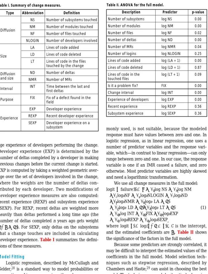
Change diffusion or interaction measures include the total number of files (NF), number of modules (NM), and number of subsystems (NS) touched by an IMR, or the number of developers involved in com-pleting an IMR (NLOGIN). We use the following IMR size measures: number of lines of code (LOC) added (LA), LOC deleted (LD), and LOC in the files touched by the change (LT). The number of MRs (NMR) and the number of deltas (ND) reflect both the diffusion and size of an IMR. We measured the duration of an IMR by calculating the difference in time between the last and first delta (INT). We also used information about whether the change was made to fix a defect found in the field (FIX). If the IMR was a fix, the pre-dictor FIX is one; otherwise it is zero.
aver-age experience of developers performing the change. Developer experience (EXP) is determined by the number of deltas completed by a developer in making previous changes before the current change is started. EXP is computed by taking a weighted geometric aver-age over the set of developers involved in the change, where the weights are the number of deltas con-tributed by each developer. Two modifications of developer experience measures are also computed: recent experience (REXP) and subsystem experience (SEXP). For REXP, recent deltas are weighted more heavily than deltas performed a long time ago (the number of deltas completed n years ago gets weight ). For SEXP, only deltas on the subsystems that a change touches are included in calculating developer experience. Table I summarizes the
defini-tions of these measures.
Model Fitting
Logistic regression, described by McCullagh and Nelder,28 is a standard way to model probabilities or proportions. Linear regression, though more
com-monly used, is not suitable, because the modeled response must have values between zero and one. In logistic regression, as in linear regression, one uses a number of predictor variables and the response vari-able, which—in contrast to linear regression—can only range between zero and one. In our case, the response variable is one if an IMR caused a failure, and zero otherwise. Most predictor variables are highly skewed and need a logarithmic transformation.
We use all change measures in the full model:
(1)
,
where , C is the intercept,
and the estimated coefficients are αi. Table II shows
the significance of the factors in the full model.
Because some predictors are strongly correlated, it may be difficult to interpret the estimated values of the coefficients in the full model. Model selection tech-niques such as stepwise regression, described by Chambers and Hastie,29can assist in choosing the best model. The technique proceeds by iteratively dropping
logit1p25log5p
/
112p26 1 a13log REXP1 a14log SEXP1a12log EXP 1 a11FIX 1 a10log INT 1a9log 1LT112 1 a8log 1LD112 1a6log NMR1 a7log 1LA112
1a3log NF1 a4log NLOGIN1 a5log ND
logit1P1failure22 5C1 a1log NS1 a2log NM
1
/
1n112Type Abbreviation Definition
Diffusion
NS Number of subsystems touched
NM Number of modules touched
NF Number of files touched NLOGIN Number of developers involved
Size
LA Lines of code added LD Lines of code deleted LT Lines of code in the files
touched by the change
Diffusion ND Number of deltas
and size NMR Number of MRs
Interval INT Time between the last and
first deltas
Purpose FIX Fix of a defect found in the
field
Experience
EXP Developer experience REXP Recent developer experience SEXP Developer experience on a
subsystem
Table I. Summary of change measures.
Description Predictor p-value
Number of subsystems log NS 0.00
Number of modules log NM 0.00
Number of files log NF 0.02
Number of deltas log ND 0.00
Number of MRs log NMR 0.04
Number of logins log NLOGIN 0.25
Lines of code added log (LA + 1) 0.00
Lines of code deleted log (LD + 1) 0.87
Lines of code in the log (LT + 1) 0.09
touched files
Is it a problem fix? FIX 0.00
Change interval log INT 0.00
Experience of developers log EXP 0.00
Recent experience log REXP 0.56
Subsystem experience log SEXP 0.36
predictors from the full model until dropping any remaining predictor would no longer be beneficial, based on Mallows Cp criteria.30,31 The procedure in this case suggested a simpler model, as follows:
(2)
Both Table II and TableIII show that the
coeffi-cients for size, diffusion, purpose, and experience are significantly different from zero, supporting our main hypothesis that change properties do affect the proba-bility of failure, at least in the considered project.
Our specific hypotheses on size and diffusion of changes are also supported because the IMR failure probability increases with the number of deltas, the number of lines of code added, and the number of subsystems touched. Average programmer experience significantly decreases the failure probability. Finally, the changes that fix field problems are more likely to fail than other IMRs if values for other predictors are comparable.
The model also indicates that the IMR interval has an influence on failure probability, even after account-ing for other factors. We speculate that the longer interval might indicate organizational or other difficul-ties that may arise when IMR is implemented, and these difficulties might increase the potential for failure. For example, if it takes an unexpectedly long time to complete coding the change, that increase could reduce the time and effort used for inspection and testing.
We should note that there may be other predictors we did not measure. For example, we expect that the number and type of installations for the SU would influ-ence the probability of failure. When an update is sent to a very large number of installations or to installations
that handle an extremely heavy workload, it is reason-able to expect the probability of failure to increase.
As a caution, note that the hypotheses were con-firmed only in a statistical sense; our statistical model (or, indeed, any statistical model) does not prove causal relationships. There might be a latent factor that affects both the predictors and the response. Since the final model is intuitive and reasonable, the possibility of such an unknown latent factor appears unlikely.
Prediction
In practice, we need to identify the IMRs that have a high risk of failure early enough in the devel-opment process to be able to take appropriate preven-tive action. Our goal is to perform the prediction immediately after the coding is complete.
Although calculating the probability of an IMR failure is an essential part of the prediction problem, we need to know what range of probability values is too high for a given delivery, so an appropriate risk management action can be taken. Furthermore, to manage the risk of an IMR, it is important to know why the model predicts a high probability of failure. We took the following steps to address these two requirements.
First, we considered the predictive power of the model by looking at a family of type I and type II errors. We then chose two cutoff probabilities to classify the IMRs into three categories: high risk, medium risk, and normal. Finally, we constructed flags, each corre-sponding to one predictor in the model, to indicate why the risk was high. For example, an IMR may be classified as having a high risk with two flags, “many subsystems touched” and “is a field fault fix.” The project management and developers responsible for the IMR then act based on the class of risk and the flags. Predictive Power
We classify an IMR as risky if its predicted probabil-ity of failure is above a cutoff value. Choosing a cutoff value means attaining a balance between two factors:
• The proportion of IMRs that do not fail when included in the SU, but are identified as risky. This proportion is categorized as the type I error. Such IMRs incur wasted effort in trying to reduce their risk.
1a6log 1LA112.
1a3FIX1 a4log INT1 a5log EXP
logit1P1failure22 5C1 a1log NS1 a2log ND
Description Predictor Estimate p-value
Number of subsystems log NS 0.41 0.000
Number of deltas log ND 0.10 0.000
Is it a fix? FIX 0.60 0.000
Interval log INT 0.05 0.000
Experience log EXP –0.11 0.002
Lines of code added log (LA + 1) 0.18 0.002
• The proportion of IMRs that do fail when included in the SU, but are not identified as risky, known as the type II error. Such IMRs incur failure remediation costs and customer dissatisfaction.
To choose an appropriate cutoff value, we need to look at error probabilities for a range of cutoff values
and to conduct a cost-benefit analysis. The decision may be different for different projects and for different types of deliveries. Customers do not expect SUs or patches to fail; consequently, the cutoff value should be lower than it would be for large deliveries like new releases of software. High-reliability systems (such as the project under study) may require lower cutoff
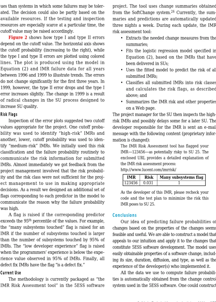
val-1.0 0.8 0.6 0.4 0.2 0.0 0.01 0.02 0.03 0.04 T ype I and T ype II errors Cutoff value 1.0 0.8 0.6 0.4 0.2 0.0 0.01 0.02 0.03 0.04 T ype I and T ype II errors Cutoff value 1.0 0.8 0.6 0.4 0.2 0.0 0.01 0.02 0.03 0.04 T ype I and T ype II errors Cutoff value 1.0 0.8 0.6 0.4 0.2 0.0 0.01 0.02 0.03 0.04 T ype I and T ype II errors Cutoff value 1996 1997 1998 1999 Type I error Type II error Figure 2.
ues than systems in which some failures may be toler-ated. The decision could also be partly based on the available resources. If the testing and inspection resources are especially scarce at a particular time, the cutoff value may be raised accordingly.
Figure 2 shows how type I and type II errors
depend on the cutoff value. The horizontal axis shows the cutoff probability (increasing to the right), while the type I and type II errors are plotted using colored lines. The plot is produced using the model in Equation (2) and IMR failure data for all years between 1996 and 1999 to illustrate trends. The errors do not change significantly for the first three years. In 1999, however, the type II error drops and the type I error increases slightly. The change in 1999 is a result of radical changes in the SU process designed to increase SU quality.
Risk Flags
Inspection of the error plots suggested two cutoff values appropriate for the project. One cutoff proba-bility was used to identify “high-risk” IMRs and another, lower, cutoff probability was used to iden-tify “medium-risk” IMRs. We initially used this risk classification and the failure probability routinely to communicate the risk information for submitted IMRs. Almost immediately we got feedback from the project management involved that the risk probabil-ity and the risk class were not sufficient for the proj-ect management to use in making appropriate decisions. As a result we designed an additional set of flags corresponding to each predictor in the model to communicate the reason why the failure probability was high.
A flag is raised if the corresponding predictor exceeds the 95thpercentile of the values. For example,
the “many subsystems touched” flag is raised for an IMR if the number of subsystems touched is larger than the number of subsystems touched by 95% of IMRs. The “low developer experience” flag is raised when the programmers’ experience is below the expe-rience value observed in 95% of IMRs. Finally, all defect fix IMRs have the flag “is a defect fix.”
Current Use
The methodology is currently packaged as “the IMR Risk Assessment tool” in the 5ESS software
project. The tool uses change summaries obtained from the SoftChange system.26 Currently, the sum-maries and predictions are automatically updated three nights a week. During each update, the IMR risk assessment tool:
• Extracts the needed change measures from the summaries;
• Fits the logistic regression model specified in Equation (2), based on the IMRs that have been delivered in SUs;
• Uses the fitted model to predict the risk of all submitted IMRs;
• Classifies all submitted IMRs into risk classes and calculates the risk flags, as described above; and
• Summarizes the IMR risk and other properties on a Web page.
The project manager for the SU then inspects the high-risk IMRs and possibly delays some for a later SU. The developer responsible for the IMR is sent an e-mail message with the following content (proprietary infor-mation is changed):
The IMR Risk Assessment tool has flagged your IMR—123456—as potentially risky to SU 25. The enclosed URL provides a detailed explanation of the IMR risk assessment process:
http://www.lucent.com/imrrisk/
As the developer of this IMR, please recheck your code and the test plan to minimize the risk this IMR poses to SU 25.
Conclusions
Our idea of predicting failure probabilities of changes based on the properties of the changes seems feasible and useful. We are able to construct a model that appeals to our intuition and apply it to the changes that constitute 5ESS software development. The model uses easily obtainable properties of a software change, includ-ing its size, duration, diffusion, and type, as well as the experience of the developer(s) who implemented it.
All the data we use to compute failure probabili-ties is automatically obtained from the change control system used in the 5ESS software. One could construct
Many subsystems flag IMR Risk
1 123456 0.031
a similar model for any software development project for which the same types of data are available, as they are likely to be for most change control systems. Even in cases where all the data are not available, it is likely that one could construct a useful failure probability model. Something as simple as a quantification of developer expertise, expressed as the number of deltas a developer has made to the code, is a strong predictor of change quality.
A key element in creating and statistically vali-dating a change failure probability model is the exis-tence of historical data that identifies which IMRs fail when included in an SU and which do not. Without such data we could not perform the logistic regression needed to construct the model. This increases the value of conducting the part of root cause analysis that identifies the changes that caused each failure.
Once the model is in place, the development organization can start using it to make decisions. Should the development organization expend resources on remedial work to improve their confi-dence that a change with a high probability of failure is safe to deliver to customers in a SU? Determining the cutoff value used to decide which IMRs receive further scrutiny is a subjective decision about balanc-ing development resources against customer satisfac-tion. Setting a high cutoff value increases the incidence of failures and angers customers; setting a low one wastes resources. Somewhat paradoxically, the decisions made about the cutoff value and about how the failure probability model is used affect the model. When all works well, the incidence of failures drops because of the increased scrutiny of high-risk changes. The lower failure incidence becomes part of the historical record on which the model is based, and the model will have to be adjusted to take the new factor into account.
It is important to note that we worked only with existing data in constructing the model—that is, we did not require the collection of any additional data about changes, and we did not perturb the change manage-ment system. Compared to the cost of maintaining the change management system, the incremental cost of computing the model is negligible. Indeed, a
consider-able amount of valuconsider-able information can be derived free from change management systems for those orga-nizations that have the discipline to use it, as illustrated in studies conducted by Basili and Weiss,26Mockus et al.,27Graves et al.,12Eick et al.,32Mockus and Votta,33 Atkins et al.,34and Siy and Mockus.35The information is free to those who have the data.
Acknowledgments
We thank our colleagues Susan K. Niedorowski, Janet L. Ronchetti, Jiyi A. Yau, and Mary L. Zajac for their support and help in starting the IMR risk identifi-cation program. We also thank Tracy Graves, Harvey P. Siy, Jonathan Y. Chen, and Tippure S. Sundresh for their contributions in the early stages of the risk identification project.
References
1. K. E. Martersteck and A. E. Spencer, Jr., “ The 5ESS†Switching System: Introduction,” AT&T Tech. J., Vol. 64, No. 6, Part 2, July–Aug. 1985, pp. 1305–1314.
2. K. H. An, D. A. Gustafson, and A. C. Melton, “A model for software maintenance,” Proc. of the Conf. on Soft. Maintenance, Austin, Texas, Sept. 21–24, 1987, IEEE Comp. Soc. Press, pp. 57–62.
3. V. R. Basili and B. T. Perricone, “Software Errors and Complexity: An Empirical Investigation,” Commun. of the ACM, Vol. 27, No. 1, Jan. 1984, pp. 42–52.
4. L. Hatton, “Reexamining the Fault Density-Component Size Connection,” IEEE Soft., Vol. 14, No. 2, Mar./Apr. 1997, pp. 89–97. 5. T. J. McCabe, “Complexity Measure,” IEEE
Trans. on Soft. Eng., Vol. SE-2, No. 4, July 1976, pp. 308–320.
6. M. H. Halstead, Elements of Software Science, Elsevier North-Holland, New York, 1977. 7. N. F. Schneidewind and H.-M. Hoffman,
“An Experiment in Software Error Data Collection and Analysis,” IEEE Trans. on Soft. Eng., Vol. SE-5, No. 3, May 1979, pp. 276–286. 8. N. Ohlsson and H. Alberg, “Predicting
Fault-Prone Software Modules in Telephone Switches,” IEEE Trans. on Soft. Eng., Vol. 22, No. 12, Dec. 1996, pp. 886–894.
9. V. Y. Shen, T.-J. Yu, S. M. Thebaut, and L. R. Paulsen, “Identifying Error-Prone Soft-ware—An Empirical Study,” IEEE Trans. on Soft. Eng., Vol. SE-11, No. 4, Apr. 1985, pp. 317–325. 10. J. C. Munson and T. M. Khoshgoftaar,
25. L. A. Belady and M. M. Lehman, “A model of large program development,” IBM Sys. J., Vol. 15, No. 3, 1976, pp. 225–253.
26. V. R. Basili and D. M. Weiss, “Evaluating Soft-ware Development by Analysis of Changes,” IEEE Trans. on Soft. Eng., Vol. SE-11, No. 2, Feb. 1985, pp. 157–168.
27. A. Mockus, S. G. Eick, T. L. Graves, and A. F. Karr, “On Measurement and Analysis of Software Changes,” Doc. No. ITD-99-36760F, BL0113590-990401-06TM, Lucent Techno-logies, Murray Hill, N. J., Apr. 1999.
28. P. McCullagh and J. A. Nelder, Generalized Linear Models, 2nded., Chapman and Hall, New York,
1989.
29. J. M. Chambers and T. J. Hastie, eds., Statistical Models in S, Wadsworth & Brooks, Pacific Grove, Calif., 1992.
30. A. J. Miller, Subset Selection in Regression, Chapman and Hall, London, 1990.
31. C. L. Mallows, “Some Comments on Cp,” Technometrics, Vol. 15, No. 4, Nov. 1973, pp. 661–667.
32. S. G. Eick, T. L. Graves, A. F. Karr, J. S. Marron, and A. Mockus, “Does Code Decay? Assessing the Evidence from Change Management Data,” IEEE Trans. on Soft. Eng. (forthcoming 2000). 33. A. Mockus and L. G. Votta, “Identifying reasons
for software changes using historic databases,” Proc. Intl. Conf. on Software Maintenance, San Jose, Calif., Oct. 11–14, 2000.
34. D. Atkins, T. Ball, T. Graves, and A. Mockus, “Using version control data to evaluate the impact of software tools,” Proc. 21stIntl. Conf. on
Soft. Eng., Los Angeles, Calif., May 16–22, 1999, ACM Press, pp. 324–333.
35. H. Siy and A. Mockus, “Measuring domain engineering effects on software change cost,” Metrics ‘99: Sixth Intl. Symp. on Soft. Metrics, Boca Raton, Fla., Nov. 4–6, 1999, pp. 304–311.
(Manuscript approved May 2000)
AUDRIS MOCKUS, a member of technical staff in the Software Production Research Department at Bell Labs in Naperville, Illinois, holds B.S. and M.S. degrees in applied mathematics from the Moscow Institute of Physics and Technology, as well as M.S. and Ph.D. degrees in statistics from Carnegie Mellon University in Pittsburgh, Pennsylvania. In his research of complex dynamic systems, Dr. Mockus designs data mining methods, data visualization techniques, statistical mod-els, and optimization techniques. He is currently
investi-Empirical investigation,” Information and Soft. Tech., Vol. 32, No. 2, Feb. 1990, pp. 106–114. 11. T.-J. Yu, V. Y. Shen, and H. E. Dunsmore,
“An Analysis of Several Software Defect Models,” IEEE Trans. on Soft. Eng., Vol. 14, No. 9,
Sept. 1988, pp. 1261–1270.
12. T. L. Graves, A. F. Karr, J. S. Marron, and H. Siy, “Predicting Fault Incidence Using Soft-ware Change History,” IEEE Trans. on Soft. Eng., Vol. 26, No. 2 (forthcoming 2000).
13. J. D. Musa, A. Iannino, and K. Okumoto, Software Reliability: Measurement, Prediction, and Application, McGraw-Hill, New York, 1990. 14. J. Jelinski and P. B. Moranda, “Software
relia-bility research,” Probabilistic Models for Software, edited by W. Freiberger, Academic Press, New York, 1972, pp. 485–502.
15. G. J. Schick and R. W. Wolverton, “An Analysis of Competing Software Reliability Models,” IEEE Trans. on Soft. Eng., Vol. SE-4, No. 2, Mar. 1978, pp. 104–120.
16. S. N. Mohanty, “Models and Measurements for Quality Assessment of Software,” ACM Computing Surveys, Vol. 11, No. 3, Sept. 1979, pp. 257–275.
17. S. G. Eick, C. R. Loader, M. D. Long, L. G. Votta, and S. Vander Wiel, “Estimating software fault content before coding,” Proc. of the 14thIntl. Conf.
on Soft. Eng., Melbourne, Australia, May 11–15, 1992, pp. 59–65.
18. D. A. Christenson and S. T. Huang, “Estimating the Fault Content of Software Using the Fix-on-Fix Model,” Bell Labs Tech. J., Vol. 1, No. 1, Summer 1996, pp. 130–137.
19. A. L. Goel, “Software Reliability Models: Assumptions, Limitations, and Applicability,” IEEE Trans. on Soft. Eng., Vol. SE-11, No. 12, Dec. 1985, pp. 1411–1423.
20. P. B. Moranda, “Software quality technology,” IEEE Comp., Vol. 11, No. 11, Nov. 1978, pp. 72–78.
21. A. K. Midha, “Software Configuration Manage-ment for the 21stCentury,” Bell Labs Tech. J.,
Vol. 2, No. 1, Winter 1997, pp. 154–165. 22. M. J. Rochkind, “The Source Code Control
System,” IEEE Trans. on Soft. Eng., Vol. SE-1, No. 4, Dec. 1975, pp. 364–370.
23. S. R. Chidamber and C. F. Kemerer, “A Metrics Suite for Object Oriented Design,” IEEE Trans. on Soft. Eng., Vol. 20, No. 6, June 1994, pp. 476–493. 24. A. J. Albrecht and J. E. Gaffney, Jr.,
“Soft-ware Function, Source Lines of Code, and Development Effort Prediction: A Software Science Validation,” IEEE Trans. on Soft. Eng., Vol. SE-9, No. 6, Nov. 1983, pp. 639–648.
gating properties of software changes in large soft-ware systems.
DAVID M. WEISS is director of Software Production Research at Bell Labs in Naperville, Illinois. He received a B.S. degree in mathematics from Union College in Schenectady, New York, and M.S. and Ph.D. degrees in computer science from the University of Maryland in College Park. Dr. Weiss directs research in the areas of software product lines, domain engineer-ing, measurement, and software architecture and specification.◆