Data-driven uncertainty quantification for predictive subsurface flow and transport modeling

(1)

Copyright by Jiachuan He

(2)

The Dissertation Committee for Jiachuan He

certifies that this is the approved version of the following dissertation:

Data-driven uncertainty quantification for predictive

subsurface flow and transport modeling

Committee:

Clint Dawson, Supervisor Tan Bui-Thanh

Omar Ghattas Chad Landis

(3)

Data-driven uncertainty quantification for predictive

subsurface flow and transport modeling

by

Jiachuan He

DISSERTATION

Presented to the Faculty of the Graduate School of The University of Texas at Austin

in Partial Fulfillment of the Requirements

for the Degree of

DOCTOR OF PHILOSOPHY

THE UNIVERSITY OF TEXAS AT AUSTIN December 2018

(4)

(5)

Acknowledgments

First and foremost, I want to express my deepest appreciation to my advisor, Prof. Clint N. Dawson, for his unremitting guidance, unwavering sup-port and continuous encouragement over the past years. He offered me great opportunities to broaden my knowledge in engineering science and to purse the research that interested me. This work benefits from his profound insights in the areas of subsurface flow modeling and uncertainty quantification. I truly enjoyed the individual weekly discussions with him which helped me develop my research topics. I am grateful for the invaluable encouragement and help he gave me to complete the work near the end of my study.

I would like to thank Professors Tan Bui-Thanh, Omar Ghattas, and Chad Landis for serving my dissertation committee. Reading Professor Tan Bui-Thanh’s notes, “A Gentle Tutorial on Statistical Inversion using the Bayesian Paradigm”, and taking Professor Omar Ghattas’ Computational and Varia-tional Methods for Inverse Problem class helped me broaden and deepen my knowledge in various aspects of solving inverse problems and quantifying un-certainty.

I would also like to thank Dr. Steven Mattis and Professor Troy But-ler for their guidance and discussions on measure-theoretic stochastic inverse problems. I wish to thank Dr. Velimir Vesselinov, my mentor during my

(6)

sum-mer internship at Los Alamos National Laboratory, for sparking my interest in applying machine learning methods to solve subsurface flow problems.

I am thankful for every member in the Computational Hydraulics Group. My thanks are extended to my friends in Austin, in particular, Jing Ping, Ju Liu, Wei Du, Peng Wang, Yimin Zhong, Hailong Xiao, Bin Wang and Zhen Tao.

I am indebted to my parents for always believing in me. Nothing is possible without their unconditional love.

(7)

Data-driven uncertainty quantification for predictive

subsurface flow and transport modeling

Publication No.

Jiachuan He, Ph.D.

The University of Texas at Austin, 2018 Supervisor: Clint Dawson

Specification of hydraulic conductivity as a model parameter in ground-water flow and transport equations is an essential step in predictive simula-tions. It is often infeasible in practice to characterize this model parameter at all points in space due to complex hydrogeological environments leading to significant parameter uncertainties. Quantifying these uncertainties requires the formulation and solution of an inverse problem using data correspond-ing to observable model responses. Several types of inverse problems may be formulated under various physical and statistical assumptions on the model parameters, model response, and the data. Solutions to most types of inverse problems require large numbers of model evaluations. In this study, we in-corporate the use of surrogate models based on support vector machines to increase the number of samples used in approximating a solution to an inverse problem at a relatively low computational cost. To test the global capabil-ities of this type of surrogate model for quantifying uncertainties, we use a

(8)

framework for constructing pullback and push-forward probability measures to study the data-to-parameter-to-prediction propagation of uncertainties un-der minimal statistical assumptions. Additionally, we demonstrate that it is possible to build a support vector machine using relatively low-dimensional representations of the hydraulic conductivity to propagate distributions. The numerical examples further demonstrate that we can make reliable probabilis-tic predictions of contaminant concentration at spatial locations corresponding to data not used in the solution to the inverse problem.

This dissertation is based on the article entitledData-driven uncertainty quantification for predictive flow and transport modeling using support vector machines by Jiachuan He, Steven Mattis, Troy Butler and Clint Dawson [32]. This material is based upon work supported by the U.S. Department of Energy Office of Science, Office of Advanced Scientific Computing Research, Applied Mathematics program under Award Number DE-SC0009286 as part of the DiaMonD Multifaceted Mathematics Integrated Capability Center.

(9)

6.1 Construction of a pullback measure from concentration obser-vation . . . 62 6.2 Validation with push-forward measure . . . 66 6.3 Concentration data-to-parameter-to-concentration prediction . 69 6.4 Head data-to-parameter-to-head prediction . . . 72 6.5 Head data-to-parameter-to-concentration prediction . . . 80

Chapter 7. Conclusions 82

Bibliography 84

(11)

List of Tables

4.1 Optimum (P, γ) for RBF kernels from coarse grid search . . . 49 4.2 Optimum (P, γ) for RBF kernels from fine grid search . . . 50 6.1 Total variations of pullback probability measures for example 2. 68 6.2 Total variations of pullback probability measures for example 3. 72 6.3 Optimum (P, γ) for RBF kernels from coarse grid search for

example 4 . . . 73 6.4 Optimum (P, γ) for RBF kernels from fine grid search for

ex-ample 4 . . . 77 6.5 Total variations of pullback probability measures for validation 77 6.6 Total variations of pullback probability measures for hydraulic

(12)

List of Figures

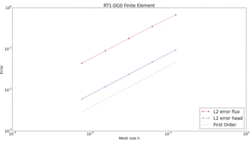
2.1 Hydraulic head . . . 20 2.2 Flux . . . 20 2.3 Error against mesh size . . . 21 3.1 A schematic figure showing streamline diffusion and crosswind

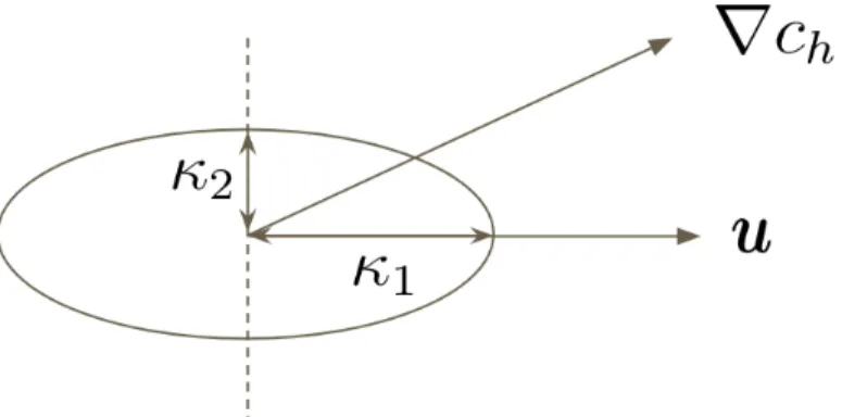
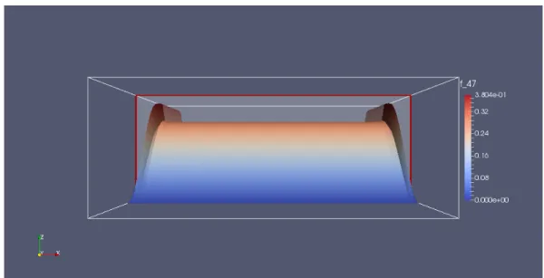
diffusion whereκ1 =κ+1₂αh|u|andκ2 =κ+₂1αech|R(ch)|/|∇ch|. 30 3.2 SUPG solution at T = 0.3 . . . 32 3.3 Slice of SUPG solution at y= 0.5 at T = 0.3 . . . 33 3.4 SUPG with crosswind diffusion solution at T = 0.3 . . . 33 3.5 Slice of SUPG with crosswind diffusion solution at y = 0.5 at

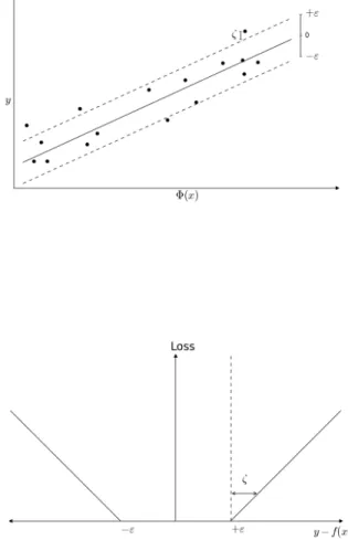
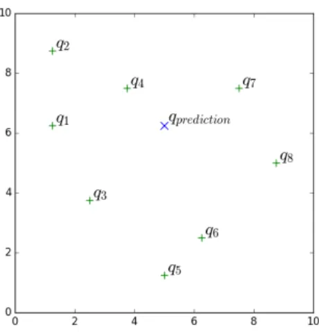
T = 0.3 . . . 34 4.1 A schematic of ε-insensitive loss function . . . 39 4.2 The flow domain. 8 green + are the only measurement locations

where contaminant concentrations are available; Blue × is the prediction location where concentration is predicted. . . 41 4.3 Range and distribution of q1. Dataset of 5000 samples (top)

and dataset of 1000 samples (bottom). . . 44 4.4 Illustration of grid search on (P, γ). Pairs of values at the grid

nodes are tried, and the one with the best cross-validation ac-curacy is picked to train the whole training set. . . 45 4.5 Scatter plots of computed concentrations at pairs of qi . . . . 47 4.6 Learning curves of the SVM surrogate for q4(ξ). . . 48 5.1 Illustrations of the inverse problem for a general two-to-one map

Left: The set-valued inverse of a single output value. Mid-dle: The representation of L as a transverse parameterization. Right: A probability measure described as a density onDmaps uniquely to a probability density on L. Figures adopted from [9] 55 5.2 The error in the µΞ−volume of a Voronoi coverage of Q−1(Dk)

affects PΞ estimation. For any fixed partitioning of D, PΞ,N converges to PΞ asN −→ ∞. . . 58

(13)

6.1 The reference lnK field approximated by a truncated KLE with 9 terms. . . 63 6.2 Samples of lnK from Voronoi cells with highest probability that

are qualitatively similar to the reference lnK . . . 65 6.3 Samples of lnK from Voronoi cells with highest probability that

are qualitatively different from the reference lnK . . . 66 6.4 Predicted probability density function of concentration at q3

using 500000 samples. The true observation at q3 is illustrated by a black dot on the x-axis. . . 69 6.5 Contours of the more realistic reference lnK field approximated

by a truncated KLE with 100 terms . . . 71 6.6 Predicted probability density of concentration at the prediction

location using 500000 samples. The reference concentration is illustrated by a black dot on the x-axis. . . 71 6.7 Scatter plots of computed concentrations at pairs of qi . . . . 75 6.8 Range and distribution of hydraulic head atq1. Dataset of 5000

samples (top) and dataset of 1000 samples (bottom). . . 76 6.9 Learning curves of the SVM surrogate for hydraulic head data

q4(ξ). . . 78 6.10 Predicted probability density function of head atq3using 500000

samples. The true observation atq3 is illustrated by a black dot on the x-axis. . . 79 6.11 Predicted probability density of head at the prediction location

using 500000 samples. The reference head is illustrated by a black dot on the x-axis. . . 80 6.12 Predicted probability density of concentration at the prediction

location using 500000 samples. The reference concentration is illustrated by a black dot on the x-axis. . . 81

(14)

Chapter 1 Introduction

1

1.1 Motivation

In the past century, demand for clean groundwater has soared due to population growth and pollution of surface water. In some areas of the world, groundwater has become the main drinking water supply or even the sole source of water. Unfortunately, contrary to the popular impression that pumping groundwater from wells and spring water is untainted, we find con-tamination of aquifers and groundwater a serious problem in many parts of the world [21, 50, 60].

Several years ago, a hexavalent chromium plume was present above the New Mexico groundwater standard of 50 parts per billion in 4 monitoring wells in the regional aquifer beneath Los Alamos National Laboratory (LANL). There is an urgent need for migration control of the chromium plume and best cleanup method assessment. Many theoretical and computational frameworks have been developed to model subsurface flow and contaminant transport [4, 22, 63, 65]. A lot of research also has been done to advance critical

decision-1_{This chapter is based on the article entitled} _{Data-driven uncertainty quantification for}

predictive flow and transport modeling using support vector machinesby Jiachuan He, Steven Mattis, Troy Butler and Clint Dawson [32].

(15)

making related to remediation strategies with uncertainties in models [8, 31, 37, 54]. Overall, prediction and remediation of subsurface require us to solve a series of mathematical problems among which we first wish to estimate unknown parameter field, e.g., hydraulic conductivity, that characterizes a model of the system. In other words, given experimental or observable data, we need to solve an inverse problem.

1.2 Background

Mathematical models for groundwater contaminant transport simula-tion often contain parameters that cannot be directly measured. Instead, we must often infer parameter values by formulating and solving an inverse prob-lem using data corresponding to observable model responses. However, a main theoretical difficulty is that most inverse problems are not well-posed in the sense of existence, uniqueness, and stability of the solution. Complicating matters further is the practical issue that solving inverse problems is often computationally intensive.

The high computational cost in solving an inverse problem may arise from many sources including the thousands or millions of forward simula-tions required, inverting large dense operators, or strong nonlinearities in the parameter-to-observable map even when the forward problem is linear. A number of recently developed methods have focused on constructing surrogate models for improved computational efficiency. A surrogate model can be re-garded as a response surface approximation of the parameter-to-observables

(16)

map defined by the composition of an observation operator with the solution operator to the model. There are many ways to construct surrogate models. For example, some popular surrogate models are based on Polynomial Chaos Expansions [46, 68], the Probabilistic Collocation Method [62, 71], Kriging [6], or Radial Basis Functions [57, 58], to name just a few. In this work, we in-corporate the use of a Support Vector Machine (SVM) which has found a wide range of applications in the fields of classification and regression analysis [5, 30]. There are also a few applications of SVM in hydrology [1, 27, 38, 43, 69]. We apply SVM to approximate the parameter-to-observable map using sets of input-output pairs of sampled model parameters and simulated model observ-ables, where the sampled model parameters define a parameterization of an unknown hydraulic conductivity field and model observables correspond to a sparse set of spatially sampled contaminant concentrations.

Using an SVM, like any surrogate, to quantify uncertainties, repre-sents a trade-off in errors where stochastic sources of error (e.g., due to finite sampling) are reduced while deterministic sources of error (e.g., due to ap-proximation errors) may be significantly increased. It is therefore important to study how accurately any surrogate can be used in quantifying uncertain-ties in both inverse and forward uncertainty quantification (UQ) problems. In general, we first solve inverse UQ problems to quantify uncertainties in model parameters, which are subsequently used to inform forward UQ problems to quantify uncertainties in model predictions. Thus, we focus first on the ability of the SVM to solve a data-to-parameter (i.e., inverse) UQ problem.

(17)

In the hydrology community, many inversion methods have been pro-posed and developed independently [72] for characterizing hydraulic conduc-tivityK[19, 36, 52], which is often the most dominant hydraulic property. The earliest method is the so-called direct method, which is relatively straightfor-ward and has been widely used [48, 49]. Assuming hydraulic head is known, one can substitute head into the forward problem and then solve the inverse problem in terms of a partial differential equation in K. However, this approach has two main shortcomings. First, this method requires the information of hy-draulic head over the entire domain. Although values of head can be achieved through interpolation of observations, it inevitably introduces smoothing of the data and errors. Second, this method is unstable due to the ill-posedness of inverse problems that small errors in head may result in large changes in the solution. To overcome these problems, indirect methods were developed to handle limited numbers of observations. Optimal parameters are found by minimizing an objective function which includes a regularization term to en-sure stability of the optimization problem. Recently, Bayesian inversion meth-ods have gained popularity in hydrologic studies [7, 24, 41, 51, 64, 67]. This approach allows a flexible integration of prior knowledge about parameters into the solution. Such a probabilistic approach is often preferable in practical problems since its solution also quantifies the uncertainties in the reconstruc-tion. However, such an approach requires additional statistical assumptions (e.g., the specification of a prior and the likelihood function, etc.), which may influence solutions, sometimes in undesirable ways [56]. Moreover, these

(18)

ap-proaches are generally focused on parameter estimation under uncertainty, and surrogate models generally need to be point-wise accurate only near a nominal parameter value (e.g., the maximum likelihood parameter) in order to obtain accurate posterior distributions, e.g., see [46].

In this work, we consider a general framework for constructing pullback and push-forward probability measures. Since constructing these measures re-quires global accuracy in the SVM, this serves as a robust test of the ability of an SVM to quantify uncertainties for other types of inverse problems. This framework is based upon the general measure-theoretic framework for the for-mulation and solution to stochastic inverse problems studied in [10]. The methodology has been successfully applied to a variety of UQ problems in storm surge modeling [28], subsurface contaminant transport [47], and struc-tural damage of vibrating beams[14]. In this study, we specify a probability measure on the observable contaminant concentration data, and through global sampling of the parameter space, we construct a pullback probability measure on the parameters defining hydraulic conductivity. We can verify that a pull-back measure was accurately computed by using the parameter-to-observable map to compute its push-forward measure and comparing it to the specified probability measure on these observables. Then, we may use this measure to construct other push-forward measures for quantities of interest (QoI) to be predicted by the model, e.g., contaminant levels at spatial locations not used in the construction of the pullback measure.

(19)

and Chapter 3, we describe the groundwater flow and contaminant transport model, and the parameterization of the hydraulic conductivity field which is the unknown parameter in the model. We provide a brief description of the fundamental principle of SVM for constructing surrogate models in Chapter 4 followed by details for constructing the SVM used in this particular work. The UQ framework for constructing pullback and push-forward probability mea-sures is summarized in Chapter 5. We present numerical examples in Chapter 6 to demonstrate the effectiveness of the proposed methodology. Finally, some concluding remarks are provided in Chapter 7.

(20)

Chapter 2 Groundwater Flow Model

Groundwater often refers to the water held underground in soils or pores that are fully saturated. Since the natural subsurface system cannot be analyzed directly because of the complex hydrogeological environment, scien-tist and engineers often use models to describe it. In this chapter, we present the mathematical model that governs groundwater flow based on mass con-servation and Darcy’s law. To solve the model, hydraulic properties including specific storage and hydraulic conductivity, which can be highly variable some-times, need to be assigned. However, in practice it’s infeasible to have direct measurements of the whole hydraulic property field. Many techniques have been proposed which can be categorized into two main approaches: Empir-ical and Experimental. The empirEmpir-ical approach is based on the correlation between hydraulic conductivity and known soil properties from other stud-ies. It calculates the hydraulic conductivity using empirical formulae such as Kozeny-Carman equation [2, 18], Hazen equation [17, 39], Breyer equation [53], etc. The experimental approach determines hydraulic conductivity through hydraulic experiments, e.g., laboratory tests and field tests. Having some sparse observations from the tests, we try to infer the hydraulic properties such that the mathematical model reproduces the observed behavior. In this

(21)

work, assuming covariance functions characterizing the hydraulic conductiv-ity field are obtained from measurements, we treat the conductivconductiv-ity field as a random function and decompose it with a Karhunen-Lo`eve Expansion (KLE). Eigenvalues and eigenfunctions in KLE can be derived analytically in some special case or computed numerically more generally. We discretize and solve the groundwater flow model by a mixed finite element method. After solv-ing the set of equations, the hydraulic heads and flow rates can be obtained and further coupled with transport models to study contaminant transport problems.

2.1 Mass Conservation

The law of conservation of mass states that for a saturated porous medium the net mass flow rate of fluid into a control volume along with sources or sinks inside is equal to the change in fluid mass storage for a given increment of time. The resulting continuity equation can be written as

∂(ρφ) ∂t =− ∂(ρqx) ∂x − ∂(ρqy) ∂y − ∂(ρqz) ∂z +ρg, (2.1)

where qx, qy and qz are components of flux q in three dimensions, ρ is den-sity of fluid, φ is porosity, and g is sources or sinks. The left-hand side of Equation (2.1), ∂(ρφ)_∂t , can be expanded as the sum of φ∂ρ_∂t and ρ∂φ_∂t. These two terms represent the produced mass rate of fluid caused by a change in hy-draulic head that leads to fluid density change and the porosity change of the porous medium, respectively. The first term is determined by the compress-ibility of the fluid while the second term is controlled by the compresscompress-ibility

(22)

of the porous media. To simplifyφ∂ρ_∂t on the left of Equation (2.1), we define the specific storage, Ss, as the volume of fluid produced under unit decline in head due to the fact that both fluid density and porosity changes are caused by the change in hydraulic head. Therefore, the mass rate of fluid produced can be written as ρSs∂h_∂t, and Equation (2.1) becomes

ρSs

∂h

∂t =−∇ ·(ρq) +ρg. (2.2)

By the chain rule, the first term on the right-hand side is the sum of−∇ρ·qand

−ρ∇ ·q. Since the magnitude of the variation in density of fluid is negligible compared to the flux divergence term, Equation (2.2) can be simplified to

Ss

∂h

∂t =−∇ ·q+g. (2.3)

2.2 Darcy’s Law

Darcy’s law is an empirical law that describes flow through a porous media. The experiment on water filtration through sand beds carried out by Darcy in 1856 showed that the gradient of hydraulic head drives the fluid from high hydraulic head to low hydraulic head. Darcy’s law can be written in differential form as

q =−K∇h, (2.4)

where q is the Darcy flux, K is hydraulic conductivity, and h is hydraulic head.

(23)

2.3 Hydraulic Conductivity Field

Hydraulic conductivity is a property of a porous medium that describes how easily a fluid can move through it. For example, hydraulic conductivity has higher values for sand or gravel compared with that for clay. In a heteroge-neous geologic formation, hydraulic conductivity is a function of position. We treat the hydraulic conductivity, K, in Equation (2.4) as a random function. In other words, nominally, the parameterK belongs to an infinite-dimensional space.

Truncating a Karhunen-Lo`eve Expansion (KLE) is a classical option for deriving finite-dimensional parameterizations for lnK. Here, we summa-rize some of the pertinent details and refer the interested reader to [26, 44] for more information. Constructing the KLE first requires specification of a covariance function. This may be obtained, for instance, assuming a station-ary random field and using a variogram on available data from a sparse set of boreholes. To ensure positive definiteness of the hydraulic conductivity, we often construct the KLE ofY(x, ω) whereY(x, ω) := ln[K(x, ω)],xis the po-sition vector defined over the domainD, andω belongs to the space of random eventsΩ. Let ¯Y(x) denote the expected value ofY(x, ω) over all possible real-izations of the process, andC(x1,x2) denote its covariance function (not to be confused with the contaminant concentrationc(x, t) in Equation (3.2)). Being an autocovariance function, C(x1,x2) is bounded, symmetric, and positive

(24)

definite. Thus, it has the spectral decomposition C(x1,x2) = ∞ X n=1 λnfn(x1)fn(x2) (2.5)

where λn and fn(x) are the solutions to the homogeneous Fredholm integral equation of the second kind:

Z

D

C(x1,x2)fn(x1)dx1 =λnfn(x2). (2.6)

The eigenfunctions are orthogonal and form a complete set. They can be normalized according to the following criterion

Z

D

fn(x)fm(x) =δnm. (2.7) Hence, Y(x, ω) can be written as

Y(x, ω) = ¯Y(x) + ∞ X n=1 ξn(ω) p λnfn(x), (2.8) whereλn and fn(x) are determined by C(x1,x2), and {ξn(ω)} is a set of ran-dom variables that can be inferred from observations. The KLE of a Gaussian field has the further property thatξn(ω) are independent standard normal ran-dom variables [40]. Truncating the series in Equation (2.8) at the Nth term gives the finite-dimensional approximation

Y(x, ω)≈Y¯(x) + N X n=1 ξn(ω) p λnfn(x). (2.9) The uncertain log hydraulic conductivity field is represented as weighted sums of predefined spatially variable basis functions. The truncated KLE provides a flexible and effective method for describing a spatially distributed hydraulic conductivity field. It reduces redundancy while capturing the most important features of the field.

(25)

2.3.1 Analytical Solution to KL expansion

The integral eigenvalue problem can be solved analytically for some special types of covariance functions defined on domains of simple geometric shape. Here we consider a one-dimensional random field characterized by an exponential covariance function. If we choose a separable covariance func-tion, the following method can be extended to multidimensional rectangular domains as Equation (2.6) can be solved in each dimension independently.

Assuming the covariance function has the form of:

C(x1, x2) = σ2Ye −|x1−x2| η _, _(2.10) Equation (2.6) becomes σ_Y2 Z L 0 e− |x₁−x₂| η f(x 2)dx2 =λf(x1). (2.11) After differentiating Equation (2.11) with respect to x1 by Leibniz rule, we have −σ 2 Y η Z x1 0 ex2 −x1 η f(x 2)dx2+ σ2 Y η Z L x1 ex1 −x2 η f(x 2)dx2 =λf0(x1). (2.12) Taking the derivative with respect tox1 again, we obtain the following equa-tion:

f00(x1) + 2ησ2

Y −λ

λη2 f(x1) = 0. (2.13) To find the boundary condition of Equation (2.13), we let x1 = 0 in Equa-tion (2.11) and EquaEqua-tion (2.12). It is then obvious that

(26)

Similarly, we can determine the other boundary condition atx1 =L

ηf0(L) = −f(L). (2.15) The general solution of Equation (2.13) has the form of

f(x) = acos(βx) +bsin(βx), where β2 = 2ησ 2 Y −λ

λη2 . (2.16) The boundary conditions require that

a−ηβb= 0 (2.17)

[−βηsin(βL) +cos(βL)]a+ [βηcos(βL) +sin(βL)]b = 0 (2.18) The homogeneous system of linear equations has a unique trivial solution if and only if the determinant of the coefficient matrix is non-zero. In order for non-trivial solutions to exist, the determinant vanishes,

(η2β2 −1)sin(βL) = 2ηβcos(βL). (2.19) There are infinitely many solutions, βn, n = 1,2,3... to Equation (2.19) in increasing order. The corresponding eigenvalues are

λn=

2ησ2_Y η2_β2

n+ 1

. (2.20)

Since fn are normalized eigenfunctions and Equation (2.16) holds, we can compute an and bn: an =ηβn 1 p (η2_β2 n+ 1)L/2 +η , (2.21) bn = 1 p (η2_β2 n+ 1)L/2 +η . (2.22)

(27)

2.3.2 Numerical Solution to KL expansion

More often, the integral equation can’t be solved analytically due to a complex geometry or a more general covariance function. Therefore, we need numerical methods for the solution of the integral eigenvalue problem. The quadrature method and Galerkin’s method are two very commonly used methods. The resulting KL expansion takes the form as:

ˆ Y(x, ω) = ¯Y(x) + N X n=1 ˆ ξn(ω) q ˆ λnfˆn(x), (2.23) where ˆλn and ˆfn(x) are approximations to the true eigenvalue and eigenfunc-tions. ˆξn(ω) are standard uncorrelated random variables.

2.3.2.1 Quadrature Method

We discretize the integral on the left-hand side of Equation (2.6) as needed for computations. The integral is approximated by numerical integra-tion:

M

X

l=1

wlCov(x,xl) ˆfn(xl), (2.24) wherexl, l= 1, ..., M are a finite set ofM quadrature points in the domain,wl is the corresponding integration weight, and ˆfn, n = 1, ..., N are approxima-tions to the true eigenfuncapproxima-tionsfn. Therefore, Equation (2.6) can be written as:

M

X

l=1

(28)

If we solve Equation (2.24) at the quadrature points, a set of equations can be formulated as:

M

X

l=1

wlCov(xm,xl) ˆfn(xl) = ˆλnfˆn(xm), m = 1, ..., M (2.26) They can be expressed in matrix form:

CWfˆ_n= ˆλnfˆn, (2.27) whereC is anM×M symmetric positive semi-definite matrix in whichcml =

Cov(xm,xl),W is a diagonal matrix with nonnegative elementswll=wl,and ˆ

f_n = ( ˆfn(x1), ...,fˆn(xM))0 is an M dimensional vector. We can then solve Equation (2.25) for the interpolation formula of the eigenfunction ˆfn(x):

ˆ fn(x) = 1 ˆ λn M X l=1 wlfˆn(xl)C(x,xl). (2.28) The KL expansion of the random field is approximated as:

ˆ Y(x, ω) = ¯Y(x) + N X n=1 ˆ ξn(ω) p ˆ λn M X l=1 wlfˆn(xl)C(x,xl) (2.29) 2.3.2.2 Galerkin Method

Galerkin methods can also be used to solve the integral equation. We let ϕl(x) be a finite set of basis functions, and expand fn(x) with respect to this basis as:

fn(x)≈fˆn(x) = M

X

l=1

(29)

Therefore, the residue of Equation (2.6) resulting from the truncated approx-imation of the eigenfunctions in Equation (2.30) is

r = M X l=1 dn_l[ Z D C(x1,x2)ϕl(x2)dx2 −λnϕl(x1)]. (2.31) According to Galerkin orthogonality, it yields a set of equations:

(r, ϕl(x)) = 0, l = 1, ..., M. (2.32) Equivalently, they can be written in matrix form:

Gdn =λnBdn, (2.33)

whereG is an M ×M matrix in which

Gml = Z D Z D C(x1,x2)ϕl(x2)dx2ϕm(x1)dx1, (2.34) B isM ×M with elements Bml = Z D ϕm(x)ϕl(x)dx. (2.35) We solve the generalized eigenvalue problem Equation 2.33 for dn and λn. Next, dn can be substituted into Equation 2.30 to obtain the approximated eigenfunctions of the covariance kernel.

2.4 Groundwater Flow Equation

Combining mass conservation and Darcy’s law, the groundwater flow model can be written as

Ss

∂h

(30)

q=−K∇h (2.37) subject to initial and boundary conditions, where Ss is specific storage, h is hydraulic head, q is flux, g is source or sink, and K is hydraulic conductivity. We consider steady groundwater flow over domain Ω with boundary,

∂Ω = Γ, that is decomposed into two parts in an incompressible saturated aquifer. The model can be simplified as:

∇ ·q=g in Ω (2.38) q=−K∇h in Ω (2.39) h=hD on ΓD (2.40) q·n=f on ΓN (2.41) Γ = ¯ΓD∪Γ¯N,ΓD∩ΓN =∅,ΓD 6=∅ (2.42) 2.4.1 Variational Formulation

We define a Hilbert space

H(div) =H(div,Ω) ={τ ∈L2(Ω;_R2)| ∇ ·τ ∈L2(Ω)}. (2.43) We let

Σg ={τ ∈H(div)|τ ·n=g on ΓN}, (2.44)

V =L2(Ω). (2.45)

Multiplying Equation (2.38) by a scalar test function v and Equation (2.39) by a vector-valued test functionτ, and then integrating over the domain Ω, we obtain a weak formulation: findq ∈Σg and h∈V such that

(31)

Z Ω ∇ ·qvdx= Z Ω gvdx ∀v ∈V, (2.46) Z Ω K−1q·τdx− Z Ω h∇ ·τdx=− Z ΓD hDτ ·nds ∀τ ∈Σ0. (2.47) The boundary condition for the flux is now an essential boundary con-dition and should be enforced in the function space, while the other boundary condition becomes a natural boundary condition, which is applied to the vari-ational form.

2.4.2 Mixed Finite Element Method

We choose finite dimensional subspaces Σh ⊂ Σ and Vh ⊂V, and the statement of the problem becomes: Find qh _∈_Σh

g, hh ∈Vh such that Z Ω ∇ ·qhvhdx= Z Ω gvhdx ∀vh ∈Vh, (2.48) Z Ω K−1qh·τhdx− Z Ω hh∇ ·τhdx=− Z ΓD hDτh·nds ∀τh ∈Σh0. (2.49) Several mixed finite element spaces may be considered, including the RTN spaces, BDM spaces, BDFM spaces, BDDF spaces, or CD spaces, to obtain a stable method.

2.4.3 Convergence Test

We consider the problem on a square domain, Ω = (0,10)×(0,10). We construct a triangular mesh of D with n elements in each direction. We let

(32)

f =− 1

4π

2_sin₍π

2y)(8cos(πx)cos(2πx)

−17sin(2πx)sin(πx)

−8sin(2πx)cos(πy)

−21sin(2πx)cos(2πy)

−55sin(2πx)).

(2.51)

We impose Dirichlet conditions of hD = 0 on the left and right boundaries. On the top and bottom boundaries

q·n= 0 (2.52)

and

q·n=−π

2(3.0 +sin(πx) +cos(2πy))sin(2πx), (2.53) respectively. The exact solutions to this simple case are:

he =sin(2πx)sin(

π

2y), (2.54)

and q_e =K∇he.

We choose Raviart-Thomas elements of order 1 for Σh, and piecewise constant for Vh. The numerical solution is obtained by using the FEniCS package. We plot the computed head and flux in Figure 2.1 and Figure 2.2. Figure 2.3 shows the discretization errors inL2 as a function of the mesh size

h. We observe that the numerical results are consistent with the finite element convergence theory that

kq_e−qhk_L2 ≤Ch, (2.55)

(33)

Figure 2.1: Hydraulic head

(34)

(35)

Chapter 3 Transport Model

Non-reactive subsurface contaminant transport in a single fluid phase can be described by a simple scalar advection-diffusion equation. However, the numerical solution to the model is still a challenge when advection is dominant. Many methods have been developed to avoid spurious oscillations. In this chapter, we first use the streamline upwind Petrov Galerkin (SUPG) method which stabilizes the numerical solution but still exhibits local oscilla-tions in crosswind direcoscilla-tions when gradients of the contaminant concentration are large. A nonlinear crosswind dissipation is then added to the SUPG for-mulation as an additional stabilization. The resulting nonlinear scheme can be solved by using linearizion through simple iteration. We show a numerical ex-ample to demonstrate the additional crosswind diffusion damps the overshoots of the SUPG solution.

3.1 Advection Diffusion Equation

Transport of solutes in porous medium can be described by conservation of mass. It states that the net rate of change of mass of solute within a control volume equals sum of the net flux of solute into the control volume

(36)

and sources/sinks inside the control volume. Advection and diffusion are two components of solute movement. The former is the transport of solute caused by the flowing groundwater that carries the solute. The latter describes the process of dispersion due to molecular diffusion. Mathematical descriptions of solute transport can be written as

u= q

φ (3.1)

∂c

∂t +∇ ·(uc)− ∇ ·(κ∇c) =f in Ω, (3.2)

wherec is the solute concentration,u is the velocity field, κ is the diffusivity and f is the source. We assume the following boundary conditions associated with Equation (3.2)

c=g on ΓD, (3.3)

κ∇c·n= 0 on ΓN, (3.4)

whereg is a given function, andn is the unit normal vector at the boundary. The initial condition is imposed as:

c(x,0) =c0(x) in Ω. (3.5) 3.1.1 Semi-Discrete Galerkin Method

We define the space of trial solutions S and the space of weighting functionsV as:

(37)

V ={w∈H1(Ω)|w= 0 on ΓD} (3.7) Multiplying Equation (3.2) by a test functionw and integrating by parts, we have the variational formulation of Equation (3.2): Findc∈S, such that

Z Ω w∂c ∂tdΩ− Z Ω ∇w·uc+∇w·(κ∇c)dΩ = Z Ω wf dΩ ∀w∈V (3.8)

Assume we have a finite element partition of the domain Ω. LetSh ⊂S

and Vh ⊂V be finite-dimensional trial solution and test function spaces.

Sh ={ch(·, t)∈H1(Ω)|ch =g on ΓD} (3.9)

Vh ={wh ∈H1(Ω)|wh = 0 on ΓD} (3.10) The Galerkin approximation formulation of Equation (3.8) can be stated as: Findch ∈Sh,such that

Z Ω wh∂c h ∂t dΩ− Z Ω ∇wh·uhch+∇wh·(κh∇ch)dΩ = Z Ω whfhdΩ ∀wh ∈Vh (3.11)

or, in an abstract compact form,

(wh, ch_t) +BG(wh, ch) = L(wh) ∀wh ∈Vh (3.12) where BG(wh, ch) :=− Z Ω ∇wh·uhch+∇wh ·(κh∇ch)dΩ (3.13) L(wh) := Z Ω whfhdΩ (3.14)

(38)

The trial solution and weighting function are continuous functions written as: ch(x, t) = N X i=1 ci(t)Ni(x), (3.15) wh(x) N X i=1 wiNi(x), (3.16)

whereNi is the standard nodal basis of Sh.

The problem above can be formulated in matrix form:

Mc˙(t) +Kc(t) =f(t), (3.17) where the dot represents the time derivative. cis the vector of time-dependent nodal values ofch_.

Mij = (Ni, Nj), (3.18)

Kij =BG(Ni, Nj), (3.19)

fi =L(Ni). (3.20)

Various numerical schemes can be applied to solve the above ordinary differential equation.

3.1.2 Semi-Discrete Stabilized Method

When the Peclet number increases, the flow becomes advection dom-inated. Solving the advection-diffusion equation by the standard Galerkin method results in unphysical oscillation of the numerical solution. To remedy the spurious oscillations, we use Steamline Upwind Petrov-Galerkin (SUPG)

(39)

method to solve the equation. In SUPG, artificial diffusion is added over el-ement interiors along the steamline direction to increase the stability of the solution. The resulting scheme can be written as: Findch _∈_Sh_, _{such that}

Z Ω wh∂c h ∂t dΩ− Z Ω ∇wh·uch+∇wh·(κ∇ch)dΩ + Nel X e=1 Z Ωe τSU P Gu· ∇whR(ch)dΩ = Z Ω whf dΩ ∀wh ∈Vh (3.21) or, (wh, ch_t) +BG(wh, ch) + Nel X e=1 (τSU P Gu· ∇wh, R(ch))Ωe =L(wh) ∀wh ∈Vh, (3.22) where R(ch) := ∂c h ∂t +∇ ·(uc h )− ∇ ·(κ∇ch)−f, (3.23) τSU P G = αh 2|u| (3.24) α=cothγ− 1 γ (3.25) γ = |u|h 2κ (3.26)

This method has strong consistency as the terms added to the standard Galerkin method vanish for all sufficiently smooth solutions.

The semidiscrete equation is a system of ODE’s

(40)

where Mij = (Ni, Nj) + Nel X e=1 (τSU P Gu· ∇Ni, Nj), (3.28) Kij =BG(Ni, Nj) + Nel X e=1 (τSU P Gu· ∇Ni,∇ ·(uNj)− ∇ ·(κ∇Nj)), (3.29) fi =L(Ni) + (τSU P Gu· ∇Ni, f). (3.30) 3.1.3 Time Integration

There are many numerical methods available to solve the following sys-tems of ordinary differential equations by advancing transient solutions step-by-step,

Mc˙(t) +Kc(t) =f(t). (3.31) Linear multistep methods and Runge-Kutta methods are two main categories of numerical methods for solving first-order initial value problem. Further-more, we can divide them into two groups that are explicit or implicit. For ex-ample, Adams-Moulton methods and backward differentiation methods (BDF) are implicit linear multistep methods, whereas diagonally implicit Runge-Kutta (DIRK), singly diagonally implicit runge kutta (SDIRK), and Gauss-Radau (based on Gaussian quadrature) numerical methods are implicit Runge-Kutta methods. Explicit linear multistep methods include the Adams-Bashforth methods. The most well known member of the Runge-Kutta family, RK4, and a generalization of the RK4 method are explicit methods. In this work, we use the standard θ− method to fully discretize the Equation (3.31) into a linear

(41)

system of algebraic equations as

(M +θ∆tK)cn+1 =θ∆tfn+1+ (1−θ)∆tfn+ (M −(1−θ)∆tK)cn (3.32) where ∆t = tn+1 −tn is the time step, and 0 ≤ θ ≤ 1 is a real parameter. When θ = 0 and θ = 1, the scheme becomes the explicit forward Euler and implicit backward Euler scheme, respectively, which both give the first-order accuracy. For θ = 1

2, it is the second-order unconditionally stable Crank-Nicolson method.

3.1.4 Crosswind-dissipation

3.1.4.1 Discontinuity-capturing crosswind-dissipation

In some cases where the solution has sharp gradients, the SUPG formu-lation alone does not completely remove the oscilformu-lations. The discontinuity-capturing technique, also known as the shock-discontinuity-capturing, is proposed to cir-cumvent this problem by introducing more numerical diffusion into the system besides the streamline diffusion. In the literature, various researchers have de-veloped several shock-captureing methods [33, 42, 55, 61]. In this work, we use the method proposed in [20] which is less diffusive than other such methods. It keeps the artificial diffusion the same as that in the SUPG formulation along the direction of the steamlines, and adds extra modified crosswind diffusion properly. Specifically, we let uk be the projection of u onto ∇ch, which is defined as

uk =

u· ∇ch

|∇ch|2

(42)

when |∇ch| is nonzero. The corresponding element Peclet number can be computed as γ_ke = uk h 2κ (3.34) γe

k is small in the regions where |u· ∇ch| is small.

The crosswind diffusion added to the left-hand side of Equation SUPG can be described as ASC(ch;wh, ch) := Nel X e=1 Z Ωe 1 2α e che |R(ch)| |∇ch| ∇wh·(I− 1 |u|2u⊗u)· ∇chdΩ (3.35)

whereI is the unit tensor. The functionαe

c is defined as

αe_c =max{0, C− 1

γe

k

}, (3.36)

whereC is an empirical constant which is often set to be 0.7 in 2D problems for linear elements. It is obvious that the crosswind diffusion is proportional to the residual defined within each element. Therefore, the consistency property still holds. Moreover, when |u· ∇ch| is small, αec will take a value close or equal to 0. That means less or no crosswind diffusion will be add to the regions where the convective term of the residual is small, which improves the accuracy of this method. In Figure 3.1, we show the artificial diffusion added in the streamline and crosswind directions in a 2D case.

The crosswind diffusion defined in Equation (3.35) is nonlinear. Non-linear methods like Newton-GMRES can be applied to solve the resulting nonlinear algebraic system.

(43)

Figure 3.1: A schematic figure showing streamline diffusion and crosswind diffusion whereκ1 =κ+1₂αh|u| and κ2 =κ+₂1αech|R(ch)|/|∇ch|.

3.1.4.2 Linearization of the nonlinear problem

As noted, the crosswind diffusion defined in Equation (3.35) is nonlin-ear. As an alternative to the nonlinear methods used in [61], we use a simple two-iteration method to solve the nonlinear equation at a low computational cost. At each time step, we first solve the transport equation by SUPG for

ch_{SU P G}: (wh,∂c h SU P G ∂t ) +BG(w h , ch_{SU P G}) + Nel X e=1 (τSU P Gu· ∇wh, R(chSU P G))Ωe =L(wh) ∀wh ∈Vh (3.37)

(44)

In the second iteration, we determine the magnitude of the crosswind diffusion based on the solutionch

SU P G and solve the linearized equation for ch: (wh,∂c h ∂t ) +BG(w h_{, c}h₎ + Nel X e=1 (τSU P Gu· ∇wh, R(ch))Ωe +A_SC(ch_{SU P G};wh, ch) =L(wh) ∀wh ∈Vh (3.38) where ASC(chSU P G;w h , ch) = Nel X e=1 Z Ωe 1 2α e ch e R(ch_{SU P G}) ∇ch_{SU P G} ∇wh·(I− 1 |u|2u⊗u)· ∇c h dΩ (3.39) 3.1.4.3 Numerical example

We consider a transport problem in Ω = (0,1)×(0,1) with homogeneous Dirichlet boundary conditions. We assume the solute concentration is zero everywhere at the initial time. The model parameters are taken asu= (0,1),

κ= 10−8, and f = 1. We solve the problem within FEniCS using continuous piecewise linear elements for spatial discretization on a uniform triangular mesh of 65×65 and the backward Euler method with a uniform time step of 10−2 _{for time integration. We integrate in time until} _T _{= 0}_._3.

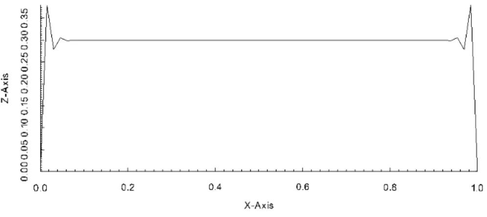
Figure 3.2 and Figure 3.3 show contours of the solutions at T = 0.3 which are computed using SUPG with and without crosswind diffusion. From the figures, it is observed that in the SUPG solution there are localized os-cillations near the boundaries where the gradient of the solution is sharp. In

(45)

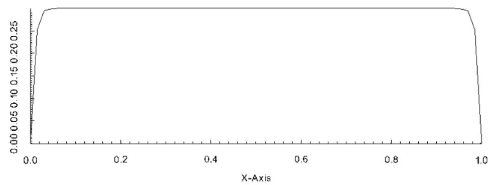
Figure 3.4 and Figure 3.5, we see that those spurious oscillations are suppressed with the application of the crosswind diffusion.

(46)

Figure 3.3: Slice of SUPG solution at y= 0.5 at T = 0.3

(47)

Figure 3.5: Slice of SUPG with crosswind diffusion solution at y = 0.5 at

(48)

Chapter 4 Surrogate Model

1

It is often computationally expensive to solve an inverse problem. One of the high computational cost may come from thousands of forward simula-tion evaluasimula-tions. To improve the efficiency, several types of surrogate models have been studied to replace expensive physics model simulations. In this chapter, we use Support Vector Machine (SVM) to build surrogate models to approximate a response surface between model parameters and a quantity of interest. Based on a small set of sampled data obtained by solving the forward problem with randomly chosen inputs, SVM surrogate models can be built to predict model output (quantity of interest) of an unseen input (model param-eters). Compared with a true model solve, computational cost associated with a surrogate model evaluation is negligible.

4.1 Surrogate Modeling with Support Vector Machines

The theory of SVM was developed based on statistical learning theory for the purpose of classification, and later extended for regression [66]. Suppose

1_{This chapter is based on the article entitled} _{Data-driven uncertainty quantification for}

(49)

we are given a set of l training points, {(x1, y1), ...,(xl, yl)}, where xi ∈ Rn is an input vector and yi ∈ R1 is the target output. The solution to the regression problems define the SVM to approximate the relation between the input vector and the output, thereby estimating the values of the output at unsampled points in the space of the input domain.

As a first step, the input vector x is mapped to a higher dimensional feature space by a map, Φ(x). Then, the regression tries to find a function

f(x) that is within an error tolerance ofε away from the given outputs in the feature space. The regression function takes the general form:

f(x) = hw,Φ(x)i+b, (4.1) wherewis a vector in the feature space. In this case, the norm ofw indicates the flatness of the function. The regression problem can be mathematically expressed in terms of the following optimization problem:

min1 2kwk 2 +P l X i=1 (ζi+ζi∗) subject to          yi−f(xi)≤ε+ζi f(xi)−yi ≤ε+ζi∗ ζi, ζi∗ ≥0 i= 1, ..., l (4.2)

where the positive constant P determines the trade-off between the flatness of f and the amount up to which deviations larger than ε are tolerated. In other words, P determines how much large deviations are penalized in the

(50)

regression. The slack variablesζ and ζ∗ are described as ζi, ζi∗ = ( 0, if |yi−f(xi)| ≤ε |yi−f(xi)| −ε, otherwise (4.3) In other words, points inside the margin (dotted lines in Figure 4.1) do not contribute to the cost function.

The above optimization problem is usually solved in its Lagrangian dual form: max−1 2 l X i,j=1 (αi−α∗i)(αj−αj∗)hΦ(xi),Φ(xj)i −ε l X i=1 (αi+α∗i) + l X i=1 yi(αi−α∗i) subject to      Pl i=1(αi−α ∗ i) = 0, 0≤αi, α∗i ≤P, i= 1, ..., l, (4.4) whereαi andαi∗ are Lagrange multipliers. In the derivation of Equation (4.4), by setting the derivatives of the Lagrangian with respect tow to zero, we have

w =

l

X

i=1

(αi−α∗i)Φ(xi). (4.5) Thus, the regression function can be rewritten as

f(x) = l

X

i=1

(αi−α∗i)k(xi,x) +b, (4.6) wherek(xi,x) = hΦ(xi),Φ(x)iis the kernel function (not to be confused with the hydraulic conductivity K in Equation (2.37)). The values of {αi}li=1 and

{α∗_i}l

i=1 are obtained by solving the dual problem, and b can be computed by exploiting the so called Karush-Kuhn-Tucker (KKT) conditions. Also, from

(51)

the KKT condition, it follows that for all points inside the margin, the corre-spondingαi andα∗i vanish. In general, when the dimensionality ofw is higher than the number of data points, it is easier to solve the optimization problem in its dual formulation. Once the dual problem is solved, the function value at any unsampled point depends only on the inner product between Φ(x) and the points in the training set with non-zeroαi values. Moreover, working with the dual problem enables us to perform the kernel trick method. Rather than mapping the input vectors through an explicit Φ and working in the enlarged feature space, it is sufficient to know k(xi,xj). This is important because in many applications of SVMs, the dimensionality of the feature space is so high that it can easily become computationally infeasible. By using kernels, one only needs to computeK(xi,xj) for all ₂l

distinct pairsi, j in Equation (4.4). Therefore, the dimensionality of the feature space does not affect the compu-tation. Note thatw is no longer given explicitly this way. Algorithmic details for computing the values needed to evaluate Equation (4.6) are discussed by [23].

Some commonly used kernel types in SVM are linear, polynomial, sig-moid and radial basis functions; see [35] for more information. The penalty parameterP and kernel parameters are then often determined using grid search with cross-validation.

(52)

(53)

4.2 SVM for Subsurface Flow Models

In this section, a two-dimensional model of saturated flow is used to construct the SVM surrogate models used in this study. This model is also used for numerical examples in Chapter 6.

We consider steady groundwater flow over domain D = (0,10) ×

(0,10)[L2] in heterogeneous porous media; see Figure 4.2 for an illustration. We impose Dirichlet conditions ofhL = 15[L] and hR = 10[L] on the left and right boundaries, respectively. On the top and bottom boundaries, q ·n = 0[LT−1_{], where}_n_{denotes the outward directed boundary normal. We assume,} for simplicity, thatY(x, ω) = ln[K(x, ω)] is Gaussian [25, 34] with zero mean and a separable exponential covariance function,

C(x1,x2) = C(x1, y1;x2, y2) = σ2Ye

[−|x1−x2|

η₁ −

|y₁−y₂|

η₂ ]_, _(4.7)

where σ2_Y = 2, η1 = 10[L] andη2 = 4[L] are the variance and the correlation lengths of the random field. Consequently, lnKcan be expanded with the form of Equation (2.8) where eigenvalues and the corresponding eigenfunctions can be analytically determined in this case according to [70]. We use the FEniCS package [3, 45] to solve the groundwater flow and transport models for the concentration. Equation (2.36) is solved using the Raviart-Thomas mixed method on a 64× 64 mesh with triangular elements. For Equation (3.2), suppose we have geophysically reasonable parameters φ = 0.1, D = 5[L2_T−1_]. There is no contaminant in the domain at the initial time. The concentration is prescribed on the left boundary as the contaminant source, CL= 50[M L−3],

(54)

Figure 4.2: The flow domain. 8 green + are the only measurement locations where contaminant concentrations are available; Blue × is the prediction lo-cation where concentration is predicted.

and no-flow (i.e., zero Neumann) otherwise. The system is discretized in time using the Crank-Nicolson method with a time step of dt = 0.05[T], and then solved by the streamline upwind Petrov Galerkin method on the same mesh.

We use the inverse transformation method (see Chapter 2 in [59]) to transform the N(0,1) distributed random variables, ξi(ω), to U(0,1) dis-tributed random variables, so that we can define the parameter domain as the unit hypercube Ξ = [0,1]9_{. For the sake of notational simplicity, we also let} _ξ

i

denote the transformed uniform random variables. Then, any inverse transfor-mation of a point ξ = (ξ1, ξ2, ..., ξ9) ∈ Ξ realizes a log hydraulic conductivity field via Equation (2.9), and the nine-dimensional domain is mapped to an

(55)

eight-dimensional output space via the parameter-to-observables map

Q(ξ) = [q1(ξ), q2(ξ), q3(ξ), q4(ξ), q5(ξ), q6(ξ), q7(ξ), q8(ξ)],

which involves solving the flow and contaminant transport models with the corresponding K and calculating the solution at the eight observation loca-tions in the physical domain (see Figure 4.2) at T = 2[T]. We draw 5000 independent identically distributed (i.i.d.) sample points in Ξ, and compute the corresponding concentrations in D.

We use the open-source software LIBSVM [16] to construct a response approximation between ξ (input) and the contaminant concentration at each observation/prediction location, qi(ξ) (output) for i= 1, ...,8, using the 5000 model evaluations as a training set. We let ε = 0.1 in the loss function Equation (4.2).

Since the dimension of input parameters is low, the RBF kernel,

k(xi,xj) =e−γkxi−xjk

2

, (4.8)

is naturally a good choice since it can handle the nonlinear relation between input and output with less hyper-parameters compared with other kernels, e.g., polynomial kernel, see [35] for more information regarding choosing kernels. The feature space in this case is implicitly defined and infinite-dimensional. Two hyper-parameters, the penalty parameter P and γ in the RBF kernel, must be determined to construct the SVM. We use a straightforward two-step grid-search method to find the optimal hyper-parameter pair (P, γ). A coarse

(56)

and fine grid search with 10-fold cross-validation are performed on a subset of size 1000 from the training set to determine the optimal hyper-parameter pair. Using an appropriate subset of data that has similar range and distribution of target outputs as the larger training set can drastically speed up the process of hyper-parameters tuning through cross-validation. In Figure 4.3, we show plots of the range and distribution of q1(ξ) from 1000 sample points and the whole training set. Scatter plots of contaminant concentration observations at

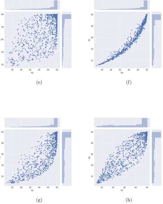
qi are shown in Figure 4.5.

Specifically, we first consider various pairs of (P, γ) values in which

P = 2−5,2−3, ...,215, and γ = 2−5,2−3, ...,215 (see Figure 4.4) on a coarse grid. For each (P, γ), we quantify its quality by performing a 10-fold cross-validation. The 1000 sample points are divided into 10 subsets of equal size. We train the model based on 9 subsets, and treat the remaining subset as an “unknown” set. The mean square error (MSE) can be computed on the “unknown” set to measure the quality of the prediction,

MSE = 1 l l X i=1 (f(xi)−yi)2, (4.9) wherel is the number of samples in the “unknown” set. The procedure is re-peated 10 times until each subset has been predicted once. The average of the 10 resulting MSE estimates indicates how accurate the model can predict un-known data. The pair that leads to the highest cross-validation accuracy (the smallest value of the average MSE) is found in Table 4.1. We then repeat the search process on a fine grid in the neighborhood of the optimal (P, γ) obtained

(57)

Figure 4.3: Range and distribution of q1. Dataset of 5000 samples (top) and dataset of 1000 samples (bottom).

(58)

Figure 4.4: Illustration of grid search on (P, γ). Pairs of values at the grid nodes are tried, and the one with the best cross-validation accuracy is picked to train the whole training set.

from the previous coarse grid search. For example, the grid-search is performed in the region of P = 211_,₂11.5_{, ...,}₂13_{, ...,}₂15_, _and _γ _{= 2}−5_,₂−4.5_{, ...,}₂−3_{, ...,}₂−1 to determine the optimal parameters for the SVM to approximate the relation betweenq1(ξ) andξ. The optimal hyper-parameters are listed in Table 4.2.

Before we build surrogate models on the whole training set including 5000 data points, we plot learning curves for a sanity check on the training set size. Learning curves plot the prediction accuracy on training and validation set against the training set size to show how the model improves at predicting the target output as we increase the number of sample points in the training set. This helps diagnose whether the model suffers from high bias or variance, and tells whether more training points will help in improving the model per-formance on prediction. If two curves converge at a low accuracy, a predictive

(59)

(a) (b)

(60)

(e) (f)

(g) (h)

(61)

Figure 4.6: Learning curves of the SVM surrogate forq4(ξ).

model is underfitting and is unable to capture the relationship between the in-put and target outin-put. Adding more training data is not helpful in this case. A more complex model is needed. If the model performs well on the training data but poorly on the validation set, i.e., there is a large gap between the two learning curves, it is overfitting. In other words, the model memorizes the data it has seen but doesn’t generalize for unseen data. We shuffle and split the whole dataset 10 times into training and validation data in the ratio of 4 to 1. Subsets of the training set with varying sizes are used to train the SVM with the hyper-parameters in Table 4.2, and MSE for each training subset size and the validation set are computed. The MSE is then averaged over all 10 runs for each training subset size. In Figure. 4.6, we show the learning curves of the surrogate model for q4. When the training set is small, the training

(62)

Table 4.1: Optimum (P, γ) for RBF kernels from coarse grid search P γ MSE R2 q1 213 2−3 0.185761369 0.957232 q2 213 2−3 0.242837426 0.952064 q3 213 2−3 0.628202705 0.966536 q4 27 2−1 1.86252441 0.964607 q5 29 2−1 3.88174606 0.957161 q6 213 2−3 4.27258069 0.967153 q7 29 2−1 5.50957803 0.971784 q8 213 2−3 5.25627116 0.975476 qprediction 213 2−3 2.27758075 0.975397

error is small too. As the training set size grows, the training error slowly increases but still remains low. On the other hand, the validation error is high due to overfitting when the model is trained on a small training set and does not generalize. Also, the large gap between training error and validation error indicates that the model trained with the given hyper-parameters in Table 4.2 exhibits high variance. In this situation, using more training points is helpful to reduce high variance. However, the validation error starts to level off when the training set size is around 4000. Including more points for training will further reduce the validation error slightly at the expense of longer training time. Therefore, in this work, we use 5000 training points to create reliable surrogate models in low computational time.

(63)

Table 4.2: Optimum (P, γ) for RBF kernels from fine grid search P γ MSE R2 q1 212 2−3 0.179665488 0.960749 q2 212 2−2.5 0.238587029 0.953566 q3 214.5 2−3.5 0.626073890 0.968131 q4 28.5 2−1.5 1.76103827 0.967289 q5 29.5 2−1 3.69977373 0.961253 q6 214.5 2−3.5 4.23652222 0.969461 q7 28 2−1 5.22852799 0.973601 q8 212 2−3 5.18621775 0.976414 qprediction 212 2−2.5 2.20208775 0.976066

(64)

Chapter 5 Measure-Theoretic Framework

1

Different types of inverse problems may be formulated under various physical and statistical assumptions on model parameters. In this chapter, we use a set-approximation method to solve the stochastic inverse problem which is formulated within a measure-theoretic framework. We consider a deter-ministic model where the dimension of the observable output is smaller than that of the model input parameters. The corresponding inverse problem then has set-valued solutions. We present a numerical method to approximate the set-valued solutions of probability measure of model input, given an assumed probability distribution on the observations.

As mentioned in Chapter 1, we focus on constructing pullback and push-forward probability measures through the surrogate defined by the SVM. By not assuming prior distributions or likelihoods, the quality of computing such probability measures is solely dependent upon the global accuracy of the SVM and its ability to propagate probabilistic events accurately.

1_{This chapter is based on the article entitled} _{Data-driven uncertainty quantification for}

(65)

5.1 Pullback and push-forward measures

We briefly describe pullback and push-forward probability measures using the notation of the previous sections. For a more thorough discussion of pullback measures including a discussion of existence and uniqueness, we direct the interested reader toA Measure-Theoretic Computational Method for Inverse Sensitivity Problems III: Multiple Quantities of Interest [10] and the references therein.

Let D = Q(Ξ) denote the range of the parameter-to-observable map and P_D a probability measure defined on D. In practice, this probability measure may be obtained by either a statistical analysis of measured data, engineering knowledge of the uncertainty in measured data, or imposed as part of an engineering design (e.g., representing worst-case scenario analysis or desired responses assuming some level of control/intervention of the model parameters Ξ). Once P_D is specified, a pullback measure PΞ on Ξ is any measure satisfying the (consistency) condition,

PΞ(Q−1(A)) =PD(A), (5.1) for every eventA inD. Oftentimes, these probability measures are described as densities ρΞ and ρD on Ξ and D, respectively, and consistency takes the form of PΞ(Q−1(A)) = Z Q−1_(A) ρΞdµΞ = Z A ρ_Ddµ_D =P_D(A), (5.2) for every event A in D, where µΞ and µD describe (volume) measures on Ξ and D, respectively.

(66)

In general, there is not a unique pullback measurePΞ since the consis-tency condition only requires specification of this measure on events Q−1₍_A₎ within Ξ. Thus, unlessQ is a bijection between Ξ and D, for any event A in D, we are free to make certain choices on how PΞ is evaluated on subsets of

Q−1₍_A_{). In Figure 5.1, we use a general two-to-one map as an example. If} _Q is a mapping from Λ ⊂ R2 _to D _⊂ _R1_{, then through the inverse map there} is a set of values, Q−1₍_Q₍_λ_{)), in Ξ that are associated to a given value} _Q₍_λ₎ where λ ∈ Λ. We call this inverse set a generalized contour. Any two points in the same generalized contour are equivalent (not distinguishable) as they correspond to the same value in D. The space of equivalence classes imposed byQ−1 _{in Λ is denoted by} _L_{, so that each point in} _L _{identifies a generalized} contour. Therefore, Q−1 _{defines a bijection map between} _L _and _D_{. To} com-pute the probability measure of any event in Ξ, we can use the Disintegration Theorem to decompose it into measures in L and along generalized contours corresponding to points inL. However, the latter is not available by inverting

Q. An Ansatz needs to be incorporated to specify the probability measures along the contours. In order to test the global accuracy of the SVM defining

Q, we use the standard Ansatz (see [10]) to proportion probabilities uniformly in directions of Ξ not informed by the map Q, hence resulting in a unique pullback measurePΞ.

Given any probability measure PΞ on Ξ, we may use the map Q to define a push-forward of this measure onD defined by

(67)

for every event A in D. Comparing Equation (5.1) and Equation (5.3), we observe that we can easily check if a pullback measure PΞ was constructed by comparing P_DQ(Ξ) with P_D on D. Moreover, by considering other maps Q

(e.g., corresponding to QoI to be predicted), we can use a pullback measure to easily construct other push-forward measures quantifying uncertainties in predictions.

(68)

Figure 5.1: Illustrations of the inverse problem for a general two-to-one map Left: The set-valued inverse of a single output value. Middle: The represen-tation of L as a transverse parameterization. Right: A probability measure described as a density on D maps uniquely to a probability density on L. Figures adopted from [9]

(69)

5.2 Numerical construction of pullback and push-forward

measures

Forward UQ problems involving the construction of push-forward mea-sures are well-studied and the meamea-sures are typically approximated using Monte Carlo or other sampling schemes. In Algorithm 1, we summarize a basic sampling scheme for approximating a pullback measure with the stan-dard Ansatz first introduced in [10]. The output of Algorithm 1 is an array of probabilities {pΞ,j}Nj=1 associated with each sample {ξ

(j)_}N

j=1 ∈Ξ. Using this array of probabilities, we can approximate the probability of any event A in Ξ using a counting measure

PΞ(A)≈PΞ,N(A) :=

X

ξ(j)∈A

pΞ,j. (5.4)

Thus, we obtain an approximation to the pullback probability measure on Ξ. This algorithm is implemented within the BET software package [29]. BET stands for Butler Estep Tavener method.

In Algorithm 1, we approximate events, implicitly, with finite collec-tions of Voronoi tessellacollec-tions of Ξ. The error of implicit Voronoi approxima-tions of Q−1₍_D

k) in Step 5 of the algorithm due to finite sampling effects the counting measure estimates. Increasing the number of samples is one of the approaches to reduce the error as shown in Figure 5.2, and with a sufficiently large number of i.i.d. samples, we often use the Monte Carlo approximation in Step 7 of the algorithm that Vj = µΞ(Ξ)/N (i.e., each Voronoi cell is ap-proximated to have the same volume). However, errors in the SVM can lead

(70)

Algorithm 1:Numerical Approximation of a Pullback Measure 1. Choose samples {ξ(j)_}N

j=1 ∈Ξ implicitly defining a Voronoi tessellation

{Vj}N

j=1 ⊂Ξ.

2. Evaluate Q(j) =Q(ξ(j)) for all ξ(j), j = 1, .., N.

3. Choose a partitioning of D,{Dk}Mk=1 ⊂D. Refer to each Dk as a bin. 4. Computep_D,k ≈PD(Dk) for k = 1, ..., M.

5. Let Ck={j|Q(j) ∈Dk} fork = 1, ..., M denote a pointer indicating the subset of {Vj}N

j=1 approximating Q

−1₍_D k). 6. Let Oj ={k|Q(j) _∈_D

k}, forj = 1, .., N denote a pointer indicating where sample Q(j) is binned in D.

7. Let Vj be the approximate volume of Vj, i.e. Vj ≈

R VjdµΞ(Vj) for j = 1, .., N. 8. Set pΞ,j = (Vj/P_i∈_C_O j Vi)pD,Oj, j = 1, .., N.

(71)

to incorrect binning of samples in Step 6 of the algorithm. These errors sub-sequently impact both pointer Ck and Oj in Steps 5 and 6 of the algorithm, respectively. Such errors propagate directly to the array of computed proba-bilities in Step 8 of the algorithm.

0 1 2 3 4 5 6 7 8 9 1 0 1 2 3 4 5 6 7 8 9 1

Figure 5.2: The error in the µΞ−volume of a Voronoi coverage of Q−1(Dk) affects PΞ estimation. For any fixed partitioning of D, PΞ,N converges to PΞ asN −→ ∞.

5.3 Comparison to Bayesian posterior and

computa-tional complexity

Here, we use some simplifying assumptions in order to provide a rea-sonable comparison between the solutions and computational complexity for inverse problems formulated in either the measure-theoretic or Bayesian frame-works. We first assume that there are no hyperparameters used in the def-initions of the prior distribution for the Bayesian formulation and that this prior is also used to formulate the Ansatz for distributing probabilities along the contour events in the measure-theoretic formulation. If we further assume that the likelihood function is defined in such a way that it matches the