HAL Id: hal-02436169
https://hal.archives-ouvertes.fr/hal-02436169
Submitted on 12 Jan 2020HAL is a multi-disciplinary open access archive for the deposit and dissemination of sci-entific research documents, whether they are pub-lished or not. The documents may come from teaching and research institutions in France or abroad, or from public or private research centers.
L’archive ouverte pluridisciplinaire HAL, est destinée au dépôt et à la diffusion de documents scientifiques de niveau recherche, publiés ou non, émanant des établissements d’enseignement et de recherche français ou étrangers, des laboratoires publics ou privés.
Trees, forests, and impurity-based variable importance
Erwan Scornet
To cite this version:
Trees, forests, and impurity-based variable
importance
Erwan Scornet
Centre de Math´ematiques Appliqu´ees, Ecole Polytechnique, CNRS, Institut Polytechnique de Paris, Palaiseau, France
Abstract
Tree ensemble methods such as random forests [Breiman,2001] are very pop-ular to handle high-dimensional tabpop-ular data sets, notably because of their good predictive accuracy. However, when machine learning is used for decision-making problems, settling for the best predictive procedures may not be reasonable since enlightened decisions require an in-depth comprehension of the algorithm pre-diction process. Unfortunately, random forests are not intrinsically interpretable since their prediction results from averaging several hundreds of decision trees. A classic approach to gain knowledge on this so-called black-box algorithm is to compute variable importances, that are employed to assess the predictive im-pact of each input variable. Variable importances are then used to rank or select variables and thus play a great role in data analysis. Nevertheless, there is no justification to use random forest variable importances in such way: we do not even know what these quantities estimate. In this paper, we analyze one of the two well-known random forest variable importances, the Mean Decrease Impu-rity (MDI). We prove that if input variables are independent and in absence of interactions, MDI provides a variance decomposition of the output, where the contribution of each variable is clearly identified. We also study models exhibit-ing dependence between input variables or interaction, for which the variable importance is intrinsically ill-defined. Our analysis shows that there may exist some benefits to use a forest compared to a single tree.
Index Terms — Random forests, variable importance, Mean Decrease Impurity, variance decomposition.
2010 Mathematics Subject Classification: 62G08, 62G20.
1
Introduction
Decision trees [see Loh, 2011, for an overview] can be used to solve pattern
recogni-tion tasks in an interpretable way: in order to build a predicrecogni-tion, trees ask to each
observation a series of questions, each one being of the form “Is variable X(j) larger
than a threshold s?” where j, s are to be determined by the algorithm. Thus the
prediction for a new observation only depends on the sequence of questions/answers for this observation. One of the most popular decision trees is the CART procedure
[Classification And Regression Trees, Breiman et al., 1984], which unfortunately suf-fers from low accuracy and intrinsic instability: modifying slightly one observation in the training set can change the entire tree structure.
To overcome this last issue, and also improve their accuracy, ensemble methods, which grow many base learners and aggregate them to predict, have been designed.
Random forests, introduced by Breiman [2001], are among the most famous tree
en-semble methods. They proceed by growing trees based on CART procedure [Breiman
et al.,1984] and randomizing both the training set and the splitting variables in each
node of the tree. Breiman’s [2001] random forests have been under active
investiga-tion during the last two decades mainly because of their good practical performance and their ability to handle high-dimensional data sets. They are acknowledged to be
state-of-the-art methods in fields such as genomics [Qi, 2012] and pattern recognition
[Rogez et al., 2008], just to name a few. If empirical performances of random forests
are not to be demonstrated anymore [Fern´andez-Delgado et al.,2014], their main flaw
relies on their lack of interpretability because their predictions result from averaging over a large number of trees (typically several hundreds): the ease of interpretation of each tree cannot be straightforwardly extended to random forests.
Since interpretability is a concept difficult to define precisely, people eager to gain insights about the driving forces at work behind random forests predictions often focus on variable importance, a measure of the influence of each input variable to predict
the output. In Breiman’s [2001] original random forests, there exist two importance
measures: the Mean Decrease Impurity [MDI, or Gini importance, seeBreiman,2002],
which sums up the gain associated to all splits performed along a given variable; and
the Mean Decrease Accuracy [MDA, or permutation importance, see Breiman, 2001]
which shuffles entries of a specific variable in the test data set and computes the difference between the error on the permuted test set and the original test set. Both measures are used in practice even if they possess several major drawbacks.
MDI is known to favor variables with many categories [see, e.g., Strobl et al.,
2007, Nicodemus, 2011]. Even when variables have the same number of categories, MDI exhibits empirical bias towards variables that possess a category having a high
frequency [Nicodemus,2011,Boulesteix et al.,2011]. MDI is also biased in presence of
correlated features [Strobl et al.,2008,Nicodemus and Malley,2009]. A promising way
to assess variable importance in random forest is based on conditional inference, via the
Rpackage party[Strobl et al.,2008,2009]. On the other hand, MDA seems to exhibit
less bias, but its scale version (the default version in the R package randomForest)
depends on the sample size and on the number of trees, the last being an arbitrary
chosen parameter [Strobl and Zeileis,2008]. The interested reader may refer toGenuer
et al. [2008] and Genuer et al. [2010] for an extensive simulation study about the influence of the number of observations, variables, and trees on MDA together with the impact of correlation on this importance measure. Despite all their shortcomings, one great advantage of MDI and MDA is their ability to take into account interaction
between features even if unable to determine the part of marginal/joint effect [Wright
et al.,2016].
From a theoretical perspective, there are only but a few results on variable
impor-tance computed via tree procedures. The starting point for theory is byIshwaran[2007]
who studies a modified version of permutation importance and derives its asymptotic positive expression, when the regression function is assumed to be piecewise constant.
[2012] who establish rate of convergence for the probability that a relevant feature is chosen in a modified random forest algorithm. The exact population expression of
permutation importance is computed byGregorutti et al.[2017] for a Gaussian linear
model.
Regarding the MDI, there are even fewer results. Louppe et al. [2013] study the
population MDI when all features are categorical. In this framework, they propose a decomposition of the total information, depending on the MDI of each variable and of interaction terms. They also prove that the MDI of an irrelevant variable is zero and that adding irrelevant variables does not impact the MDI of relevant ones. Even if these results may appear to be very simple, the proofs are not straightforward at all,
which explains the few results on this topic. This work was later extended by Sutera
et al.[2016] to the case of context-dependent features.
It is instructive to notice that there is no general result establishing the consistency of these variable importance measures toward population quantities when computed with the original random forest algorithms: all existing results focus on modified ran-dom forests version with, in some cases, strong assumptions on the regression model. Therefore, there are no guarantees that using variable importance computed via ran-dom forests is suitable to select variables, which is nevertheless often done in practice.
Agenda. In this paper, we focus on the regression framework and derive
theoreti-cal properties about the MDI used in Breiman’s [2001] random forests. Section 2 is
devoted to notations and describes tree and forest construction, together with MDI
calculation. The main results are gathered in Section 3. We prove that both
pop-ulation MDI and empirical MDI, computed with Breiman’s random forests, can be seen as a percentage of explained variance and are directly related to the quadratic risk of the forest. We also derive the expression of the sum of MDIs for two groups of variables that are independent and do not interact, which is at the core of our analysis. The analysis highlights that fully-developed random forests (whose tree leaves contain exactly one observation) produce inaccurate variable importances and should not be
used for that purpose. In Section 4, we establish that for additive regression models
with independent inputs, the MDI of each variable takes a very simple, interpretable
form, which is the variance of each univariate component mj(X(j)). We prove that
empirical MDI computed with Breiman’s forest targets this population quantity, which is nothing but a standard way to decompose the variance of the output. Hence, in the absence of input dependence and correlation, MDI computed with random forests provides a good assessment of the variable importance. To the best of our knowledge, it is the first result proving the good properties of the empirical MDI computed with Breiman’s forests. To move beyond the additive models and understand the impact
of interactions, we study a multiplicative model in Section 5. In this model, MDI is
ill-defined and one needs to aggregate many trees to obtain a consistent MDI value. Averaging trees is known to be of great importance to improve accuracy but it turns out to be mandatory to obtain consistent variable importance measure in the pres-ence of interactions. The impact of dependpres-ence between input variables is studied
in Section 6. We stress out that correlated variables are more likely to be chosen in
the splitting procedure and, as a consequence, exhibit a larger MDI than independent ones. As for the presence of interactions, this highlights the importance of computing
2
Notation and general definition
We assume to be given a data set Dn = {(Xi, Yi), i= 1, . . . , n} of i.i.d. observations
(Xi, Yi) distributed as the generic pair (X, Y) where X ∈ [0,1]d and Y ∈ R with
E[Y2]<∞. Our aim is to estimate the regression functionm : [0,1]d→R, defined as
m(X) = E[Y|X], using a random forest procedure and to identify relevant variables,
i.e. variables on whichm depends.
2.1
CART construction and empirical MDI
CART [Breiman et al.,1984] is the elementary component of random forests [Breiman,
2001]. CART construction works as follows. Each node of a single treeT is associated
with a hyper-rectangular cell included in [0,1]d. The root of the tree is [0,1]ditself and,
at each step of the tree construction, a node (or equivalently its corresponding cell) is split in two parts. The terminal nodes (or leaves), taken together, form a partition of
[0,1]d. An example of such tree and partition is depicted in Figure 1, whereas the full
procedure is described in Algorithm1.
Yes
Yes No Yes
No
No
Figure 1: A decision tree of depth k = 2 in dimension d = 2 (right) and the
corre-sponding partition (left).
We define now the CART-split criterion. To this aim, we let A ⊂ [0,1]d be a
generic cell andNn(A) be the number of data points falling into A. A split in A is a
pair (j, z), where j is a dimension in {1, . . . , d} and z is the position of the cut along
the j-th coordinate, within the limits of A. We let CA be the set of all such possible
cuts in A. Then, for any (j, z) ∈ CA, the CART-split criterion [Breiman et al., 1984]
takes the form
Ln,A(j, z) = 1 Nn(A) n X i=1 (Yi−Y¯A)21Xi∈A − 1 Nn(A) n X i=1 (Yi−Y¯AL1X(j) i <z −Y¯AR1X(j) i ≥z )21Xi∈A, (1)
whereAL={x∈A :x(j) < z}, AR ={x∈ A:x(j) ≥z}, and ¯YA (resp., ¯YAL, ¯YAR) is
the average of the Yi’s belonging to A (resp., AL, AR), with the convention 0/0 = 0.
At each cellA, the best cut (jn,A, zn,A) is finally selected by maximizingLn,A(j, z) over
CA, that is
(jn,A, zn,A)∈arg max
(j,z)∈CA
Algorithm 1CART construction.
1: Inputs: data set Dn, query point x ∈ [0,1]d, maximum number of observations
in each leaf nodesize
2: Set Aleaves =∅ and Ainner nodes={[0,1]d}.
3: while Ainner nodes6=∅ do
4: Select the first element A∈ Ainner nodes
5: if A contains more thannodesize observations then
6: Select the best split minimizing the CART-split criterion defined below (see
equation (1))
7: Split the cell accordingly.
8: Concatenate the two resulting cellAL and AR at the end of Ainner nodes.
9: Remove A fromAinner nodes
10: else
11: ConcatenateA at the end of Aleaves.
12: Remove A fromAinner nodes
13: end if 14: end while
15: For a query point x, the tree outputs the average mn(x) of the Yi falling into the
same leaf as x.
To remove ties in the argmax, the best cut is always performed along the best cut
direction jn,A, at the middle of two consecutive data points.
The Mean Decrease in Impurity (MDI) for the variable X(j) computed via a tree
T is defined by [ MDIT(X(j)) = X A∈T jn,A=j
pn,ALn,A(jn,A, zn,A), (3)
where the sum ranges over all cellsA in T that are split along variable j and pn,A is
the fraction of observations falling into A. In other words, the MDI ofX(j) computes
the weighted decrease in impurity related to splits along the variableX(j).
2.2
Theoretical CART construction and population MDI
In order to study the (empirical) MDI defined in equation (3), we first need to define
and analyze the population version of MDI. First, we define a theoretical CART tree,
as in Algorithm1, except for the splitting criterion which is replaced by its population
version. Namely, for all cellsAand all splits (j, z)∈ CA, the population version of the
CART-split criterion is defined as
L?A(j, z) =V[Y|X∈A]−P[X(j)< z|X∈A] V[Y|X(j) < z,X∈A]
−P[X(j)≥z|X∈A] V[Y|X(j)≥z,X∈A]. (4)
Therefore in each cell of a theoretical tree T?, the best split (j?
A, zA?) is chosen by
maximizing the population version of the CART-split criterion that is
(jA?, zA?)∈arg max
(j,z)∈CA
Of course, in practice, we cannot build a theoretical tree T? since it relies on the
true distribution (X, Y) which is unknown. A theoretical tree is just an abstract
mathematical object, for which we prove properties that will be later extended to the (empirical) CART tree, our true object of interest.
As for the empirical MDI defined above, the population MDI for the variableX(j)
computed via the theoretical tree T? is defined as
MDI?T?(X(j)) = X A∈T? j? A=j p?AL?A(jA?, zA?),
where all empirical quantities have been replaced by their population version and the theoretical CART tree is used instead of the empirical CART tree defined in
Section2.1. We also let p?A=P[X∈A].
Random forest A random forest is nothing but a collection of several decision trees whose construction has been randomized. In Breiman’s forest, CART procedure serves as base learner and the randomization is performed in two different ways:
1. Prior to the construction of each tree, a sample of the original data set is ran-domly drawn. Only this sample is used to build the tree. Sampling is typically
done using bootstrap, by randomly drawing n observations out of the originaln
observations with replacement.
2. Additionally, for each cell, the best split is not selected along all possible
vari-ables. Instead, for each cell, a subsample of mtryvariables is randomly selected
without replacement. The best split is selected only along these variables. By
default, mtry=d/3 in regression.
Random forest prediction is then simply the average of the predictions of such ran-domized CART trees. Similarly, the MDI computed via a forest is nothing but the average of the MDI computed via each tree of the forest.
In the sequel, we will use the theoretical random forest (forest that aggregate theoretical CART trees) and the population MDI to derive results on the empirical random forest (forest that aggregate empirical CART trees; the one widely used in practice) and the empirical MDI.
3
Main theoretical result
For any theoretical CART treeT?, and for anyk ∈N, we denote byT?
k the truncation
ofT? at level k, that is the subtree of T? rooted at [0,1]d, in which each leaf has been
cut at most k times. Let AT?
k(x) be the cell of the tree T
?
k containing x. For any
functionf : [0,1]d→R and any cell A⊂[0,1]d, let
∆(f, A) =V[f(X)|X∈A]
be the variance of the functionf in the cell A with respect to the distribution of X.
Proposition 1 states that the population MDI computed via theoretical CART trees
can be used to decompose the variance of the output, up to some residual term which depends on the risk of the theoretical tree estimate.
Proposition 1. Assume that Y =m(X) +ε, where ε is a noise satisfying E[ε|X] = 0
and V[ε|X] = σ2 almost surely, for some constant σ2. Consider a theoretical CART
treeT?. Then, for all k ≥0,
V[Y] = d X j=1 MDI?T? k(X (j)) + EX0 h V[Y|X ∈AT? k(X 0 )]i, (5)
where X0 is an i.i.d. copy of X.
Note that few assumptions are made in Proposition1, which makes it very general.
In addition, one can see that the sum of population MDI is close to the R2 measure
used to assess the quality of regression model. The populationR2 is defined as
1− EX 0 h V[Y|X∈AT? k(X 0)]i V[Y] = Pd j=1MDI ? T? k(X (j)) V[Y] .
Hence, the sum of MDI divided by the variance of the output corresponds to the
percentage of variance explained by the model, which is exactly the population R2.
Therefore, Proposition1draws a clear connection between MDI and the very classical
R2 measure.
We say that a theoretical tree T? is consistent if lim
k→∞∆(m, AT? k(X
0)) = 0. If a
theoretical tree is consistent, then its populationR2 tends toV[m(X)]/V[Y] as shown
in Corollary 1below.
Corollary 1. Grant assumptions of Proposition1. Additionally, assume thatkmk∞<
∞ and, almost surely, lim
k→∞∆(m, AT
? k(X
0)) = 0. Then, for all γ > 0, there exists K
such that, for all k > K,
d X j=1 MDI?T? k(X (j))− V[m(X)] ≤γ
Consistency (and, in this case, tree consistency) is a prerequisite when dealing with algorithm intepretability. Indeed, it is hopeless to think that we can leverage infor-mation about the true data distribution from an inconsistent algorithm, intrinsically incapable of modelling these data. Therefore, we assume in this section that theoret-ical trees are consistent and study afterwards variable importances produced by such algorithm. In the next sections, we will be able to prove tree consistency for specific regression models, allowing us to remove the generic consistency assumption in our
results, as the one in Corollary1.
Corollary1 states that if the theoretical tree T?
k is consistent, then the sum of the
MDI of all variables tends to the total amount of information of the model, that is
V[m(X)]. This gives a nice interpretation of MDI as a way to decompose the total
variance V[m(X)] across variables. Louppe et al. [2013] prove a similar result when
all features are categorical. This result was latter extended by Sutera et al. [2016]
in the case of context-dependent features. In their case, trees are finite since there exists only a finite number of variables with a finite number of categories. The major difference with our analysis is that trees we study can be grown to arbitrary depth.
We thus need to control the error of a tree stopped at some levelk, which is exactly
According to Corollary1, the sum of the MDI is the same for all consistent theoret-ical trees: even if there may exist many theorettheoret-ical trees, the sum of MDI computed for each theoretical tree tends to the same value, regardless of the considered tree. Therefore, all consistent theoretical tree produce the same asymptotic value for the sum of population MDI.
In practice, one cannot build a theoretical CART tree or compute the population
MDI. Proposition 2 below is the extension of Proposition 1 for the empirical CART
procedure. LetTn be the (empirical) CART tree built with data setDnand let, for all
k, Tn,k be the truncation of Tn at level k. Denote byV[[Y] the empirical variance ofY
computed on the data set Dn. Define, for any function f : [0,1]d 7→ R, the empirical
quadratic risk via
Rn(f) = 1 n n X i=1 (Yi−f(Xi))2.
Proposition 2 (Empirical version of Proposition 1). Let Tn be the CART tree, based
on the data set Dn. Then,
[ V[Y] = d X j=1 d MDITn(X(j)) +Rn(fTn), (6)
where fTn is the estimate associated to Tn, as defined in Algorithm 1.
Note that equations (5) and (6) in Proposition 1 and Proposition 2 are valid for
general tree construction. The main argument of the proof is simply a telescopic sum
of the MDI which links the variance ofY in the root node of the tree to the variance
of Y in each terminal node. These equalities hold for general impurity measures by
providing a relation between root impurity and leaves impurity. As in Proposition1,
Proposition2 proves that theR2 of a tree can be written as
Pd j=1MDI[Tn(X (j)) [ V[Y] , (7)
which allows us to see the sum of MDI as the percentage of variance explained by the model. This is particularly informative about the quality of the tree modelling when
the depth k of the tree is fixed.
Trees are likely to overfit when they are fully grown. Indeed, the risk of trees which
contain only one observation per leaf is exactly zero. Hence, according to equation (6),
we have [ V[Y] = d X j=1 [ MDITn(X (j))
and theR2 of such tree is equal to one. Such R2 does not mean that trees have good
generalization error but that they have enough approximation capacity to overfit the
data. Additionally, for a fully grown tree Tn, we have
lim n→∞ d X j=1 [ MDITn(X (j)) = V[m(X)] +σ2.
For fully grown trees, the sum of MDI contains not only all available information
V[m(X)] but also the noise in the data. This implies that the MDI of some variables
are higher than expected due to the noise in the data. The noise, when having a larger variance than the regression function, can induce a very important bias in the MDI by overestimating the importance of some variables. When interested by interpreting a decision tree, one must never use the MDI measures output by a fully grown tree. However, if the depth of the tree is fixed and large enough, the MDI output by the
tree provides a good estimation of the population MDI as shown in Theorem1.
Model 1. The regression model satisfies Y = m(X) +ε where m is continuous, X admits a density bounded from above and below by some positive constants and ε is an independent Gaussian noise of variance σ2.
Theorem 1. Assume Model 1holds and that for all theoretical CART tree T?, almost
surely,
lim
k→∞∆(m, AT
?
k(X)) = 0.
Let Tn be the CART tree based on the data set Dn. Then, for all γ > 0, ρ ∈ (0,1],
there exists K ∈N? such that, for all k > K, for all n large enough, with probability
at least 1−ρ, d X j=1 d MDITn,k(X(j))−V[m(X)] ≤γ.
As for Corollary1, Theorem 1 relies on the consistency of theoretical trees, which
is essential to obtain positive results on tree interpretability. It is worth noticing that
Theorem 1 is not a straightforward extension of Corollary 1. The proof is based on
the uniform consistency of theoretical trees and combines several recent results on tree partitions to establish the consistency of empirical CART tree.
It is not possible in general to make explicit the contribution of each MDI to the sum. In other words, it is not easy to find an explicit expression of the MDI of each variable. This is due to interactions and correlation between inputs, which make difficult to distinguish the impact of each variable. Nevertheless, when the regression model can be decomposed into a sum of two independent terms, we can obtain more
precise information on MDI. To this aim, let, for any setJ ={j1, . . . , jJ} ⊂ {1, . . . , d},
X(J)= (X(j1), . . . , X(jJ)).
Model 2. There exists J ⊂ {1, . . . , d} such that X(J) and X(Jc)
are independent and
Y =mJ(X(J)) +mJc(X(J c)
) +ε, (8)
where mJ and mJc are continuous functions, ε is a Gaussian noise N(0, σ2)
inde-pendent of X and X admits a density bounded from above and below by some positive constants.
Lemma 1. Assume Model 2 holds. Then, for all j ∈ J, the criterion L?A(j, s) does not depend on mJc and is equal to L?
A(J)(j, s). Besides, any split j ∈ J leaves the
variance ofmJc unchanged.
Lemma 1will be used to prove Proposition 3 below but is informative on its own.
It states that if the regression model can be decomposed as in Model 2, the best split
Proposition 3. Assume Model 2 holds. Let T?
J be a tree built on distribution (X(J),
mJ(X(J))) and let TJ?,k be the truncation of the tree at level k. Similarly, let TJ?c be
a tree built on distribution (X(Jc)
, mJc(X(J c)
)) and let T?
Jc,k be the truncation of the
tree at level k. If for any tree T?
J and TJ?c, almost surely, lim k→∞∆(mJ, AT ? J,k(X (J))) = 0, and lim k→∞∆(mJ c, AT? Jc,k(X (Jc) )) = 0
then, for any treeT? built on the original distribution (X, Y), almost surely,
lim
k→∞∆(m, AT
?
k(X)) = 0.
Proposition 3 states that the consistency of any theoretical trees results from the
consistency of all theoretical trees built on subsets (J and Jc) of the original set of
variables, under Model2. This is of particular significance for proving the consistency
of theoretical tree for a new model which can be rewritten as a sum of independent regression functions: we can then deduce the tree consistency from existing consistency results for each regression function. Note that there are no structural assumptions on
the functions mJ and mJc apart from the continuity. In particular, the class of
functions in Model2 is wider than additive functions.
Theorem2below proves that the sum of the MDI inside groups of variables that (i)
do not interact between each other and (ii) are independent of each other is well-defined
and equals the variance of the corresponding component of the regression function.
Theorem 2. Under the assumptions of Proposition 3, for all γ > 0, there exists K
such that, for all k > K, X j∈J MDI?T? k(X (j))− V[mJ(X(J))] ≤γ, and X j∈Jc MDI?T? k(X (j))− V[mJc(X(J c) )] ≤γ.
Besides, for all γ >0, ρ∈ (0,1], there exists K such that, for all k > K, for all n
large enough, with probability at least 1−ρ, X j∈J d MDITn,K(X(j))−V[mJ(X(J))] ≤γ, and X j∈Jc d MDITn,K(X (j))− V[mJc(X(J c) )] ≤γ.
Theorem 2 establishes the limiting value of the sum of MDI in subgroups J and
Jc, both for the population version and the empirical version of the MDI, as soon
as all theoretical trees are consistent. We will use Theorem 2 in the Section 4 to
derive explicit expressions for the MDI of each variable, assuming a specific form of the regression function.
4
Additive Models
One class of models particularly easy to interpret is additive models (sum of univariate functions) with independent inputs defined as below.
Model 3 (Additive model). The regression model writes
Y =
d
X
j=1
mj(X(j)) +ε,
where each mj is continuous; ε is a Gaussian noise N(0, σ2), independent of X; and
X∼ U([0,1]d).
Due to the model additivity, there is no interaction between variables: the contribu-tion of each variable for predicting the output is reduced to its marginal contribucontribu-tion. Since we also assume that features are independent, the information contained in one variable cannot be inferred by the values of other variables.
By considering a model with no interaction and with independent inputs, we know that the contribution of a variable has an intrinsic definition which does not depend on
other variables that are used to build the model. In Model 3, the explained variance
of the modelV[m(X)] takes the form
V[m(X)] =
d
X
j=1
V[mj(X(j))],
which holds only because of independent inputs and the absence of interactions. The
variance explained by the jth variable is defined unambiguously, and independently
of which variables are considered in the model, asV[mj(X(j))]. Therefore any
impor-tance measure forX(j)which aims at decomposing the explained variance must output
V[mj(X(j))]. It turns out that the MDI computed via CART trees converges to this
quantity.
Theorem 3 (Additive model). Assume that Model 3 holds. Let T? be any theoretical
CART tree and Tn be the empirical CART tree. Then, for all γ > 0, there exists K
such that, for all k > K, for all j, MDI ? T? k(X (j))− V[mj(X(j))] ≤γ,
Moreover, for all γ >0, ρ ∈ (0,1], there exists K such that, for all k > K, for all n
large enough, with probability at least 1−ρ, for all j, d MDITn,k(X(j))−V[mj(X(j))] ≤γ.
Since the MDI computed via random forests is nothing but the average of MDI
computed by trees, Theorem 3 also holds for MDI computed via random forests. To
the best of our knowledge, Theorem 3 is the first result highlighting that empirical
MDI computed with CART procedure converge to reasonable values that can be used
for variable selection, in the framework of Model3.
Contrary to Theorem 2, Theorem 3 does not assume the consistency of the
theo-retical tree. Indeed, in the context of additive models, one can directly take advantage of Scornet et al. [2015] to prove the consistency of theoretical CART trees.
Surprisingly, the population version of MDI has the same expression as the
popula-tion version of MDA (up to factor 2), as stated inGregorutti et al.[2017]. Thus, in the
particular context of additive models with independent features, both MDI and MDA target the same quantity, which is the natural way to decompose the total variance. In this context, MDI and MDA can then be employed to rank features and select variables based on the importance values they produce.
Note that MDI is computed with truncated trees, i.e. trees that contain a large number of observations in each node. This is mandatory to ensure that the variance of the output in the resulting cell is correctly estimated. As mentioned before, con-sidering fully grown trees would result in positively-biased MDI, which can lead to unintended consequences for variable selection. We therefore stress that MDI must not be computed using fully grown trees.
Theorem 3 proves that MDI computed with any CART tree are asymptotically
identical: the MDI are consistent across trees. The only interest to use many trees to compute the MDI instead of a single one relies on the variance reduction property of ensemble methods, which allows us to reduce the variance of the MDI estimate when using many trees.
Remark: invariance under monotonous transformations Tree-based meth-ods are known to be invariant by strictly monotonous transformations of each input.
Letting fj being any monotonous transformation applied to variable X(j), the new
regression model writes
Y =
d
X
j=1
mj◦fj−1(fj(X(j))) +ε,
wherefj(X(j)) are the new input variables. Assuming that Theorem3 can be applied
in the more general setting where X(j) ∼f
j(U([0,1])), the MDI for this new problem
satisfies lim k→∞MDI ? T? k(X (j)) = V[mj◦fj−1(fj(X(j)))] =V[mj(X(j))].
Therefore the asymptotic MDI is invariant by monotonic transformation, assuming
that Theorem 3 holds for any marginal distribution of X (with independent
compo-nents).
One particularly famous instance of additive models are the well-studied and ex-tensively used linear models.
Model 4 (Linear model). The regression model writes
Y =
d
X
j=1
αjX(j)+ε,
where, for all j, αj ∈ R; ε is a Gaussian noise N(0, σ2), independent of X; and
X∼ U([0,1]d).
As for Model 3, there is only one way to decompose the explained variance for
linear models with independent input, as stated byNathans et al.[2012] andGr¨omping
[2015] (and the references therein), which is α2
jV[X(j)]. Theorem 4 below proves that
MDI converge to these quantities and provides information about the theoretical tree
Theorem 4(Linear model). Assume that Model4holds. For any cellA=Qd
`=1[a`, b`]⊂
[0,1], the coordinate which maximizes the population CART-split criterion (4) satisfies
j? ∈arg max
`∈{1,...,d}
α2`(b`−a`)2
and the splitting position is the center of the cell; the associated variance reduction is
α2 j? 4 b j?−aj? 2 2 .
Let T? be any theoretical CART tree and T
n be the empirical CART tree. Then, for
all γ >0, there exists K such that, for all k > K and for all j,
MDI ? T? k(X (j))− α 2 j 12 ≤γ.
Moreover, for all γ >0, ρ ∈ (0,1], there exists K such that, for all k > K, for all n
large enough, with probability at least 1−ρ, for all j,
d MDITn,k(X (j))− α 2 j 12 ≤γ.
Theorem 4 establishes that, for linear models with independent inputs, the MDI
computed with CART trees whose depth is limited is exactly the quantity of interest,
which depends only on the magnitude ofα2
j, since all variables have the same variance.
Theorem4 is a direct consequence of Theorem3. However, for linear models, one can
compute explicitly the best splitting location and the associated variance decreasing,
which is stated in Theorem4. Being able to compute the variance decreasing for each
split allows us to compute the MDI directly, without using Theorem3. Note that the
splitting location and variance reduction has been first stated byBiau[2012] and then
byIshwaran [2013].
5
A model with interactions
In the absence of interaction and dependence between inputs, the MDI is a measure of variable importance which is independent of the set of variables included in the model,
as stated in Theorem 3. However, this is not true as soon as we consider classes of
models that present interactions or dependence. In this section, we study the influence of interactions via the following model.
Model 5 (Multiplicative model). Let α∈R. The regression model writes
Y = 2dα
d
Y
j=1
X(j)+ε.
where, for all j, αj ∈ R; ε is a Gaussian noise N(0, σ2), independent of X; and
Theorem 5 (Multiplicative model). Assume that Model 5 holds. For any cell A =
Qd
`=1[a`, b`] ⊂ [0,1], the coordinate which maximizes the population CART-split
crite-rion (4) satisfies j? ∈arg max `∈{1,...,d} b`−a` a`+b` ,
and the splitting position is the center of the cell; the associated variance reduction is
α2
4 (bj?−aj?)
2 Y
`6=j?
(a`+b`)2
Let T? be any theoretical CART tree and T
n be the empirical CART tree. Then, for
all γ >0, there exists K such that, for all k > K,
d X j=1 MDI?T? k(X (j))−α24 3 d −1 ≤γ.
Moreover, for all γ >0, ρ ∈ (0,1], there exists K such that, for all k > K, for all n
large enough, with probability at least 1−ρ,
d X j=1 d MDITn,k(X(j))−α2 4 3 d −1 ≤γ.
Theorem5gives the explicit splitting position for a model with interactions.
Deriv-ing splittDeriv-ing positions allows us to prove that the theoretical tree is consistent which,
in turns, proves that the sum of MDI converges to the explained variance V[m(X)],
according to Theorem2.
We are also interested in obtaining the exact MDI expression for each variable,
as established for additive models. However, Theorem 2 no longer applies since the
regression model cannot be decomposed into independent additive components. It turns out to be impossible to derive explicit expression for each MDI in this model.
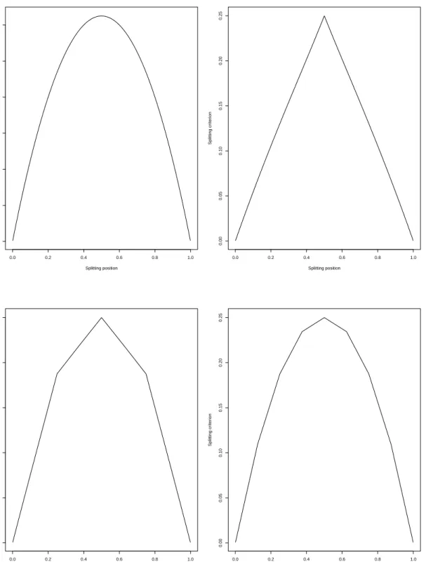
To see this, note that there exist many theoretical trees in Model 5. Two of them
are displayed in Figure 2. They result in the same partition but the first split can
be made either alongX(1) (Figure 2, left) or X(2) (Figure 2, right). Surprisingly, the
variable importance computed with these trees is larger for the variable that is split in the second step. This exemplifies that splits occurring in the first levels of trees do not lead to the largest decrease in variance. Nonetheless, this holds only when interactions
are present: in the case of the additive models defined in Section 4, the decrease in
variance is stronger in the first tree levels. A direct consequence of this fact is that two different theoretical tree can output two different variable importance, as shown
by Lemma 2below.
Lemma 2. Assume that Model 5holds. Then, there exists two theoretical trees T1 and
T2 such that lim k→∞ MDI?T 2,k(X (1))−MDI? T1,k(X (1)) =α2/16.
According to Lemma 2, there exist many different theoretical trees for Model 5
Figure 2: Two theoretical tree partitions of level k = 2: the first split is performed
alongX(1) (resp. X(2)) for the tree on the left (resp. on the right).
major difference with additive models for which each theoretical tree asymptotically output the same MDI. Since MDI are usually used to rank and select variables, the fact that each tree can output a different MDI, and therefore a different variable ranking, is a major drawback for employing this measure in presence of interactions. One way to circumvent this issue could be to compute the MDI via a random forest: the randomization of splitting variables yields different trees and the aggregation of MDI across trees provides a mean effect of the variable importance. For example, in
Model5, one can hope to obtain importance measure that are equal since Model 5 is
symmetric in all variables. This is impossible with only one tree but is a reachable goal by computing the mean of MDI across many trees as done in random forests. More generally, for simple regression problems, a single tree may be sufficient to predict accurately but many shallow trees are needed to obtain accurate MDI values.
6
A model with dependent inputs
Up until now, we have focused on independent input variables. This is often an
unrealistic assumption. To gain insights on the impact of input dependence on MDI, we study a very specific model in which input features are not independent. We will prove that even in this very simple model, MDI has some severe drawbacks that need to be addressed carefully. Accordingly, we consider the simple case where the input
vector X = (X(1), X(2)) is of dimension two and has a distribution, parametrized by
β∈N, defined as X∼ U ∪2β−1 j=0 j 2β, j+ 1 2β 2! =U⊗2β . (9)
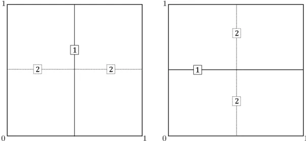
The distribution of X is uniform on 2β squares on the diagonal. Examples of such
distribution are displayed in Figure 3. For such distribution, the correlation between
Figure 3: Illustration of distributions for X, with parameter β = 1 (left) and β = 2 (right).
Lemma 3. Let X= (X(1), X(2))∼ U⊗2β as defined in (9). Then
Corr(X(1), X(2)) = 1− 1
4β.
For β = 0, the distribution of X is uniform over [0,1]2 and accordingly, the
cor-relation is null between the two components of X, as stated in Lemma 3. When β
(i.e., the number of squares) increases, that is the size of each square decreases, the
distribution concentrates on the lineX(1) =X(2). Therefore, whenβ tends to infinity,
the correlation should tend to 1, which is proved in Lemma3.
The distribution defined in (9) is rather unusual, and one can wonder why not
considering Gaussian distributions instead. This choice is related to the thresholding nature of decision trees. Since we want to compute explicitly the splitting criterion along each coordinate, we must have a closed expression for the truncated marginals
(restriction to any rectangle of [0,1]2), which is not possible with Gaussian distribution.
The distribution defined in (9) allows us to compute easily both truncated marginals
and the joint distribution.
Model 6. Let β∈N. Assume that
Y =X(1)+X(2)+αX(3)+ε,
where (X(1), X(2))∼ U⊗2β
, X(3) ∼ U([0,1]) is independent of (X(1), X(2)), and ε is an
independent noise distributed as N(0, σ2).
In the framework of Model 6, Proposition 4 below states that the CART-split
criterion has an explicit expression and highlights that splits along positively correlated
variables (X(1)andX(2)) are more likely to occur compared to splits along independent
ones (X(3)). Even if the model is very simple, it is the first theoretical proof that
CART splitting procedure tends to favor positively correlated variables. Note however
that considering negatively correlated variables will result in an opposite effect,i.e., a
tendency to favour independent variables compared to negatively correlated ones.
(i) The splitting criterion has an explicit expression. For β = 0, . . . ,5, each split is performed at the center of the support of the chosen variable.
(ii) For β= 0, . . . ,5, the split in the root node[0,1]3 is performed along X(1) or X(2)
if, and only if, |α| ≤2. In that case, the variance reduction is equal to 1/4.
Statement (ii) in Proposition 4 proves that a positive correlation between two
variables increases the probability to split along one of these two variables. Indeed,
in our particular model, the marginal effect of X(3) on the output must be at least
twice the effect of X(1) or X(2) in order to split along X(3). It is likely that the
way the correlation impact the variable selection in trees depends both on the sign of the correlation and on the signs of coefficients in the linear model. Nevertheless,
Proposition 4 proves that input dependence has an influence on variable selection in
CART procedures. Theorem 6 provides the limiting MDI values given by theoretical
and empirical CART trees, in Model 6.
Theorem 6. Letβ ∈ {0, . . . ,5}. Assume that Model 6holds. LetT? be any theoretical
CART tree and Tn be the empirical CART tree. Then, for all γ > 0, there exists K
such that, for all k > K, MDI ? T? k(X (1)) +MDI? T? k(X (2))− V[X(1)+X(2)] ≤γ. and MDI ? T? k(X (3))−α2 V[X(3)] ≤γ.
Additionally, for all γ > 0, ρ ∈(0,1], there exists K such that, for all k > K, for all
n large enough, with probability at least 1−ρ, d MDITn,k(X(1)) +MDITd n,k(X (2))− V[X(1)+X(2)] ≤γ. and d MDITn,k(X(3))−α2V[X(3)] ≤γ.
Theorem 6 gives the limiting values for the MDI. Unfortunately, since X(1) and
X(2) are correlated, it is only possible to have information on the sum of the two MDI
of X(1) and X(2) rather than on each one of them. According to Lemma 3, a simple
calculation shows that the sum of importances ofX(1) and X(2) satisfies,
V[X(1)+X(2)] = 2V[X(1)] + 2V[X(1)] 1− 1 22β >V[X(1)] +V[X(2)].
Therefore, the group of variables X(1) and X(2) has a larger importance because of
their positive correlation. In this case, the amount of information provided by the two variables is larger than that provided by each one of them. This is a very important difference compared to the independent additive case, in which the sum of contributions of each variable is equal to the contributions of all variables. Here, even without interaction effects, this property does not hold, which leads to larger MDI for variables
that are positively correlated. As mentioned before, the opposite effect would hold if the variables had a negative correlation or if they had coefficients of opposite signs in the linear model.
Even if the limiting value MDI?T?
K(X
(1)) + MDI?
T? K(X
(2)) is known, we have no
in-formation on how this quantity is split between variable X(1) and X(2) inside the tree
T?
K. Indeed, we can find two theoretical trees which produce very different MDI as
stated in Lemma 4.
Lemma 4. Let β ∈ {0, . . . ,5}. Assume that Model 6 holds. Then, there exists two theoretical trees T1 and T2 such that
lim k→∞ MDI?T 2,k(X (1))−MDI? T1,k(X (1)) = 1 3 − 1 3 1 4 β .
Even in the case of a simple linear model with correlated input, it is not wise to use the importance of a single tree to measure the impact of this variable on the output, since this measure can vary drastically between two different trees. Instead, one should rather use an average of this measure across many shallow trees, hoping that randomizing the eligible variables for splitting ensure enough tree diversity in the forest, which in turn, leads to more balanced variable importances.
The proof of Lemma4relies on exhibiting a tree whose early splits are made along
X(1) only, until X is uniformly distributed in each cell. For this tree, the importance
ofX(1) is larger than the importance ofX(2) SinceX(1)andX(2) have symmetric roles,
one can also build a tree whose early splits are made along X(2) only. The difference
of importance for X(1) between these two trees can be computed exactly, thanks to
statement (i) and (ii) in Proposition4.
7
Proofs
Proof of Proposition 1. LetT? be a theoretical CART tree and define, for all k ∈N,
the variance uk of the treeTk? (the truncation of T at levelk) as
uk = ncell,k
X
`=1
P[X∈A`,k]V[Y|X∈A`,k],
wherencell,k stands for the number of terminal nodes inTk? and{A`,k, `= 1, . . . , ncell,k}
is the set of terminal nodes in T?
k. Let fk(x) = V[Y|X0 ∈ Ak(x)]. By definition of
the impurity measure, note that, for allk, the quantity uk−uk+1 corresponds to the
reduction of impurity between levelkand level k+ 1. Therefore, the impurity measure
rewrites, for any K ∈N as
d X j=1 MDI?T? K(X (j)) = K−1 X k=0 (uk−uk+1) =u0−uK, (10)
whereu0 =V[Y] by definition. Additionally, E[fk(X)] =E ncell,k X `=1 V[Y|X0 ∈A`,k]1X∈A`,k = ncell,k X `=1 P[X ∈A`,k]V[Y|X0 ∈A`,k] =uk,
yielding the desire conclusion
d X j=1 MDI?T? K(X (j)) = V[Y]−E[fK(X)]. (11)
Proof of Corollary 1. Using notations of the proof of Proposition 1, for all x∈[0,1]d,
fk(x)≤4kmk2∞+σ2 and, by assumption, almost surely, limk→∞fk(X) =σ2.
Accord-ing to the dominated convergence theorem, lim k→∞uk = limk→∞E[fk(X)] = σ 2. Therefore, lim K→∞ d X j=1 MDI?T? K(X (j)) = V[Y]−σ2. (12)
Proof of Proposition 2. Equation (11) in the proof of Proposition1, written with em-pirical quantities, leads directly to the first statement.
Proof of Theorem 1.
Uniform convergence of theoretical trees. Note that a tree is nothing but a
sequence of splits. Therefore, any tree T can be seen as a sequence (vn) such that
• (v1, . . . , vd) represents the first split of the tree defined, for a split occurring along
variable j at position s, as
(
v` = 0 for `6=j
vj = ds4
• Each block (vmd+1, . . . , v(m+1)d) represents the mth split of the tree occurring
along variable j at position s defined as
(
v` = 0 for `6=j
vj = (d(ms+1))4
• In order to obtain a complete tree, we associate with all nodes whose construction
is stopped, the split (0, . . . ,0).
Since the split position belongs to [0,1], we have P∞`=1v2
` <∞. Besides, ∞ X `=1 `2v`2 ≤ ∞ X `=1 1 `2 = π2 6 .
For any treeT represented by the sequence (vn), we have
(vn)∈B(0, π2/6) = n v, ∞ X `=1 `2v2` ≤π2/6o,
with B(0, π2/6) being a compact of`2(N). Now, let γ >0 and
Ak,γ = n T?, E[∆(m, AT? k(X))]≥γ o
Set A∞,γ =∩∞k=0Ak,γ. Since the population CART-split criterion L?, defined in (4) is
non negative, we have
E[∆(m, ATk+1(X))]≤E[∆(m, ATk(X))].
Therefore, for allk, Ak+1,γ ⊂ Ak,γ. Because of the uniform continuity of the splitting
criterion (continuous on a compact), for all k∈N, the sets Ak,γ are closed.
Assume that for allk,Ak,γ 6=∅. We know thatB(0, π2/6) is compact and that, for
all k, Ak,γ is a closed subset of B(0, π2/6). Then, according to Cantor’s intersection
theorem A∞,γ 6= ∅. Consequently, there exists T? ∈ A∞,γ. By definition of A∞,γ, for
allk,
E[∆(m, AT?
k(X))]≥γ. (13)
Again, by definition ofA∞,γ,T?is a theoretical tree, which is consistent by assumption.
Consequently, there existsK such that, for all k > K,
E[∆(m, AT?
k(X))]≤γ,
which is absurd, according to equation (13). Therefore, there exists K > 0 such that
AK,γ = ∅. All in all, we proved that, for all γ >0, there exists K >0 such that, for
all theoretical tree T?, for all k > K,
E[∆(m, ATk(X))]< γ. (14)
Contribution of cells with small measure. Fixγand takeKsuch that inequality
(14) holds. For any theoretical tree T?
K of level K, the MDI associated with this tree
is defined as MDI?T? K = X A∈T? K µ(A)L?A,
where the sum ranges for any node A in the tree, µ(A) is the measure of the cell A
defined as
µ(A) =
Z
x∈A
where f is the density of X and L?
A the value of the population CART-split criterion
at the best split of the cell A. Similarly, we let
[
MDITn,K =
X
A∈Tn,K
µn(A)Ln,A,
where Tn,K is the empirical CART tree truncated at level K, A a node of the tree,
µn(A) the empirical measure of A and Ln,A the empirical splitting criterion in cell
A. Let MDI?T?
K,γ and MDI[Tn,K,γ be computed by removing the variance (empirical or
population version) associated to cells A for which µ(A) < γ. Define also MDI?T
n,K,γ
as the population version of the MDI but computed with the empirical partition Tn,K
where the cells A for which µ(A)< γ have been removed. Now, we want to control
inf
T? |[MDITn,K −MDI
?
T?
K| ≤ |MDI[Tn,K−MDI[Tn,K,γ|+|MDI[Tn,K,γ−MDI
? Tn,K,γ| + inf T?|MDI ? Tn,K,γ −MDI ? T? K,γ|+ infT?|MDI ? T? K,γ−MDI ? T? K|. (15)
Since X admits a density on [0,1]d, the population CART-split criterion varies
con-tinuously as a function of the cell on which it is computed. Thus, the third term in
(15) is controlled as soon as the empirical partition is close to the theoretical partition.
Lemma 3 in Scornet et al.[2015] can be easily extended for any continuous regression
functionm and any density which is bounded from above and below by some positive
constants. Therefore, with probability 1−ρ, for all n large enough,
inf T? |MDI ? Tn,K,γ−MDI ? T? K,γ| ≤γ. (16)
Last term in (15) can be treated directly by noting that the theoretical criterion is
bounded above by 4kmk2 ∞. Therefore, we have |MDI?T? K,γ−MDI ? T? K| ≤2 K+2kmk2 ∞γ. (17)
To control the second term, we make use of the results of Wager and Walther[2015],
in particular Corollary 11 which can be adapted to a Gaussian noise by noting that
with probability 1−ρ, max1≤i≤n|εi| ≤Cρlogn. Note that our setting is simpler than
that of Wager and Walther [2015] where the dimension d grows to infinity with n.
Therefore, with probability at least 1−ρ, for all n large enough,
|MDI[Tn,K,γ −MDI
?
Tn,K,γ| ≤γ. (18)
Regarding the first term in (15), for any cell A such thatµ(A)< γ,
µn(A)Vn[Y|X ∈A]≤4µn(A)kmk2∞+µn(A)Vn[ε|X ∈A].
With probability 1−ρ, for allnlarge enough, max
1≤i≤n|εi| ≤Cρlognand, ifnµn(A)≥ √ n, 1 nµn(A) X i,Xi∈A ε2i ≤2σ2.
Therefore, with probability 1−ρ, for all n large enough, 4µn(A)kmk2∞+µn(A)Vn[ε|X ∈A]≤8γkmk2∞+ Nn(A) n 1 Nn(A) X i,Xi∈A ε2i ≤8γkmk2 ∞+ 4γσ21Nn(A)≥ √ n+ Cρlogn √ n 1Nn(A)< √ n ≤8γkmk2 ∞+ 4γσ2. (19)
Injecting inequalities (16)-(19) into (15), with probability 1−ρ, for allnlarge enough,
inf T? |MDI[Tn,K−MDI ? T? K| ≤8γkmk 2 ∞+ 4γσ2+ 2γ+ 2K+2kmk2∞γ. (20) Since, |MDI[Tn,K−V[m(X)]| ≤inf T? |MDI[Tn,K−MDI ? T? K|+|MDI ? T? K −V[m(X)]|,
we conclude, from (14), (20) and Corollary 1, with probability 1−ρ, for all n large
enough,
|MDI[Tn,K −V[m(X)]| ≤3γ+ 8γkmk 2
∞+ 4γσ2+ 2K+2kmk2∞γ.
Sinceρ and γ are arbitrary, this concludes the proof.
Proof of Lemma1. Let A = Qd
j=1[aj, bj] ⊂ [0,1]d be a generic cell. Recall that the
regression model satisfies
Y =mJ(X(J)) +mJc(X(J c)
) +ε.
For allj ∈ J, and all splitting position s, define the two resulting cells
AL =A∩ {x, x(j) < s} and AR=A∩ {x, x(j)≥s},
where, for notation brevity, the dependence on j and s is omitted. The variance
reduction associated to any split (j, s) is defined as
L?A(j, s) =V[m(X)|X∈A]−P[X∈AL|X ∈A]V[m(X)|X∈AL] −P[X∈AR|X ∈A]V[m(X)|X ∈AR] =V[mJ(X(J))|X∈A]−P[X∈AL|X ∈A]V[mJ(X(J))|X∈AL] −P[X∈AR|X ∈A]V[mJ(X(J))|X ∈AR] +V[mJc(X(J c) )|X∈A]−P[X∈AL|X ∈A]V[mJc(X(J c) )|X∈AL] −P[X∈AR|X ∈A]V[mJc(X(J c) )|X∈AR].
Since the split is performed along thejth coordinate,
V[mJc(X(J c) )|X ∈AL] =V[mJc(X(J c) )|X∈AR] =V[mJc(X(J c) )|X∈A]. (21)
Consequently, the variance reduction satisfies
L?A(j, s) =V[mJ(X(J))|X∈A]−P[X∈AL|X∈A]V[mJ(X(J))|X ∈AL]