PhD thesis, University of Nottingham.
Access from the University of Nottingham repository: http://eprints.nottingham.ac.uk/12309/1/Phd_Thesis_2011.pdf Copyright and reuse:
The Nottingham ePrints service makes this work by researchers of the University of Nottingham available open access under the following conditions.
· Copyright and all moral rights to the version of the paper presented here belong to the individual author(s) and/or other copyright owners.
· To the extent reasonable and practicable the material made available in Nottingham ePrints has been checked for eligibility before being made available.
· Copies of full items can be used for personal research or study, educational, or not-for-profit purposes without prior permission or charge provided that the authors, title and full bibliographic details are credited, a hyperlink and/or URL is given for the original metadata page and the content is not changed in any way.
· Quotations or similar reproductions must be sufficiently acknowledged.
Please see our full end user licence at:
http://eprints.nottingham.ac.uk/end_user_agreement.pdf
A note on versions:
The version presented here may differ from the published version or from the version of record. If you wish to cite this item you are advised to consult the publisher’s version. Please see the repository url above for details on accessing the published version and note that access may require a subscription.
SUPER-RESOLUTION MAPPING
byANUAR MIKDAD MUAD, M.Sc.
Thesis submitted to the University of Nottingham for the degree of Doctor of Philosophy
Abstract
Super-resolution mapping is becoming an increasing important technique in remote sensing for land cover mapping at a sub-pixel scale from coarse spatial resolution imagery. The potential of this technique could increase the value of the low cost coarse spatial resolution imagery. Among many types of land cover patches that can be represented by the super-resolution mapping, the prediction of patches smaller than an image pixel is one of the most difficult. This is because of the lack of information on the existence and spatial extend of the small land cover patches. Another difficult problem is to represent the location of small patches accurately. This thesis focuses on the potential of super-resolution mapping for accurate land cover mapping, with particular emphasis on the mapping of small patches. Popular super-resolution mapping techniques such as pixel swapping and the Hopfield neural network are used as well as a new method proposed. Using a Hopfield neural network (HNN) for super-resolution mapping, the best parameters and configuration to represent land cover patches of different sizes, shapes and mosaics are investigated. In addition, it also shown how a fusion of time series coarse spatial resolution imagery, such as daily MODIS 250 m images, can aid the determination of small land cover patch locations, thus reducing the spatial variability of the representation of such patches. Results of the improved HNN using a time series images are evaluated in a series of assessments, and demonstrated to be superior in terms of mapping accuracy than that of the standard techniques. A novel super-resolution mapping technique based on halftoning concept is presented as an alternative solution for the super-resolution mapping. This new technique is able to represent more land cover patches than the standard techniques.
List of publications
1. Muad, A.M. and Foody, G.M. (2011), Super-resolution mapping of lakes from imagery with a coarse spatial and fine temporal resolution, International Journal of Applied Earth Observation and Geoinformation. In Press.
2. Muad, A.M. and Foody, G.M. (2010). Super-resolution mapping using multiple observations and Hopfield neural network. In Proceedings of the SPIE Remote Sensing, Toulouse, France, 20-23 September 2010.
3. Muad, A.M. and Foody, G.M. (2010). Super-resolution analysis for accurate mapping of land cover and land cover pattern. In Proceedings of the IEEE International Geoscience and Remote Sensing Symposium (IGARSS), Honolulu, Hawaii, USA, 25-30 July 2010.
4. Muad, A.M. and Foody, G.M. (2010). Super-resolution mapping of landscape objects from coarse spatial resolution imagery. In Proceedings of the GEOgraphic Object-Based Image Analysis (GEOBIA), Ghent, Belgium, 29 June - 2 July 2010.
Acknowledgements
First of all, I would like to express my sincere gratitude and thanks to my supervisor, Professor Giles M. Foody. I am grateful to Professor Foody for accepting me as his student and providing guidance, helps and continuous support throughout the period of this study. Without all his help and suggestions, this work would not have been possible. Thanks also to Dr. Doreen Boyd as my co-supervisor. Also, I would like to extend my gratitude and thanks to the Ministry of Higher Education of Malaysia and Universiti Kebangsaan Malaysia for sponsoring my research for a PhD degree at the University of Nottingham and getting my study leave sanctioned. I would like to convey my thanks to all the staff members at the School of Geography, University of Nottingham for their co-operation and support, especially to Jenny Ashmore, Andrea Payne, Carol Gilbourne, Ian Conway, Jonathan Walton, Louise McIntyre, and John Milner. Thanks also to post-doctorate and postgraduate students, especially Wan Hazli Wan Kadir, Dr. Mahesh Pal, Dr. Yuan-Fong Su, Dr. Nurul Islam, Sani Yahaya, Pantelis Arvanitis, and Oluwakemi Akintan for their invaluable assistance and advice as well as their friendship during this work. I wish to extend my thanks to Prof. Aini Hussain, Prof. Azah Mohamed, Prof. Marzuki Mustafa, Dr. Hafizah Husain and Mrs. Normah Adam from Universiti Kebangsaan Malaysia and Dr. Nooritawati Md. Tahir from Universiti Teknologi Mara for their kind help throughout my study. Special recognition is due to my parents, Muad Kulop Mat Alip and Jamaeyah Kamaruddin, family and relatives in Malaysia for their continuous encouragement and support. Special thanks is due to my wife, Rizamul Aili Tajuddin for her endless patience and understanding during all long hours of work that kept me busy in my research.
Table of contents
ABSTRACT ... II LIST OF PUBLICATIONS ... III ACKNOWLEDGEMENTS ... IV TABLE OF CONTENTS ... V LIST OF FIGURES ... X LIST OF TABLES ... XVIII LIST OF ABBREVIATIONS AND ACRONYMS ... XXIII
1. INTRODUCTION ... 1 1.1. Overview... 1 1.2. Objectives ... 7 1.3. Thesis structure ... 8 2. BACKGROUND ... 11 2.1. Super-resolution restitution ... 11
2.1.1. Frequency domain approach ... 12
2.1.2. Spatial domain approach ... 13
2.1.3. Motionless super-resolution ... 14
2.1.4. Recognition based super-resolution ... 15
2.1.5. Super-resolution restitution in remote sensing ... 15
2.2. Super-resolution mapping ... 16
2.2.1. Soft classification ... 16
2.2.1.1. Linear mixture model ... 17
2.2.1.2. Maximum likelihood classification ... 18
2.2.1.4. Feed-forward neural network ... 19
2.2.1.5. Support vector machine ... 20
2.2.2. Super-resolution mapping ... 21
2.2.2.1. Knowledge based procedure ... 22
2.2.2.2. Linear optimization ... 22
2.2.2.3. Feed-forward neural network ... 23
2.2.2.4. Hopfield neural network ... 23
2.2.2.5. Neural network predicted wavelet coefficients ... 25
2.2.2.6. Markov random field ... 25
2.2.2.7. Pixel swapping ... 26 2.2.2.8. Geo-statistics indicator ... 27 2.3. Accuracy assessment ... 28 2.3.1. Confusion matrix ... 28 2.3.2. Texture variables... 28 2.3.2.1. Homogeneity ... 29 2.3.2.2. Contrast ... 30
2.3.2.3. Inverse difference moment ... 31
2.3.2.4. Entropy ... 32
2.3.3. Object based characterization ... 32
2.3.4. Positional accuracy ... 34
2.4. Conclusions ... 34
3. SUPER-RESOLUTION ANALYSIS FOR MAPPING PATTERNED LANDSCAPES ... 36
3.1. Fuzzy c-means soft classification ... 36
3.2. Hopfield neural network ... 38
3.2.1. Hopfield neural network for super-resolution mapping ... 43
3.2.2. Incorporating prior information into HNN ... 48
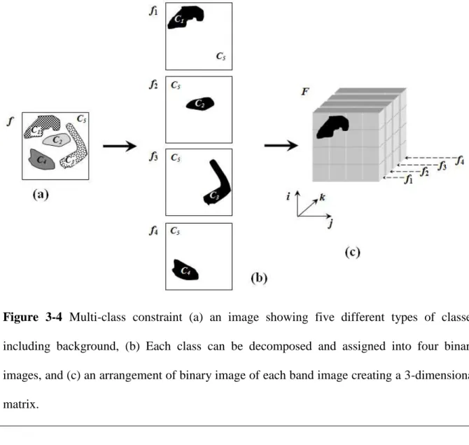
3.2.3. Multiclass land cover mapping ... 50
3.3. Pixel swapping ... 52
3.4. Experimental analysis ... 54
3.5. Conclusions ... 70
4. SUPER-RESOLUTION MAPPING FOR SMALL LAND COVER PATCHES ... 72
4.1. Introduction... 73
4.2. Sub-pixel patches in a mixed pixel ... 75
4.3. Large land cover patches ... 78
4.4. Small land cover patches ... 81
4.5. Experimental evaluation ... 83
4.6. Representation of large land cover patches with HNN ... 85
4.6.1. Weight settings ... 85
4.6.2. Number of iterations ... 89
4.7. Representation of small land cover patches with HNN ... 94
4.7.1. Weight settings ... 95
4.7.2. Number of iterations ... 97
4.8. The impact of weight settings on the HNN for the representation of small land cover patches ... 104
4.9. Representation of large land cover patches with pixel swapping ... 108
4.10. Representation of small land cover patches with pixel swapping ... 110
4.11. Representation of different mixed pixel scenarios ... 112
4.12. Conclusions ... 121
5. INCREASING THE ACCURACY OF LAND COVER PATCH LOCATION ... 123
5.1. Introduction... 123
5.2. Mis-location of small land cover patches ... 129
5.3. Image fusion from multiple observations ... 131
5.4. Sub-pixel shift estimation ... 138
5.5. Incorporating a fusion of multiple observations into super-resolution mapping140 5.6. Spatial variability analysis ... 141
5.7. Land cover patches representation using multiple coarse spatial resolution images
... 149
5.8. Conclusions ... 154
6. SUPER-RESOLUTION MAPPING FOR LANDSCAPE PATCHES USING A FUSION OF TIME SERIES IMAGERY ... 156
6.1. Introduction... 156
6.2. Moderate Resolution Imaging Spectroradiometer ... 158
6.3. Landsat ETM+ ... 159
6.4. Test site and data ... 160
6.5. Sub-pixel shift estimation in the time series MODIS images... 164
6.6. A two-step HNN for super-resolution mapping ... 165
6.7. Experimental analysis ... 167
6.7.1. Single MODIS image... 167
6.7.2. Time series MODIS images ... 169
6.7.3. Notations ... 169
6.8. Results and discussions ... 169
6.8.1. Single MODIS image... 170
6.8.1.1. Site specific thematic accuracy assessment ... 175
6.8.2. Time series MODIS images ... 181
6.8.2.1. Site specific thematic accuracy assessment ... 185
6.8.3. Texture variables... 188
6.8.4. Characterization of the shape of lakes ... 195
6.8.5. Positional accuracy ... 202
6.9. Conclusions ... 208
7. SUPER-RESOLUTION MAPPING USING THE HALFTONING CONCEPT ... 210
7.1. Introduction... 210
7.3. Methods ... 216
7.3.1. Time series image registration and data fusion ... 217
7.3.2. Halftoning ... 219
7.3.3. 2D multiple notch filter... 222
7.3.4. Iterative morphological filter ... 225
7.4. Lake characterization ... 227
7.5. Results and discussion ... 229
7.6. Conclusions ... 239 8. CONCLUSIONS ... 240 8.1. Summary ... 241 8.2. Contributions ... 244 8.3. Future works ... 245 BIBLIOGRAPHY ... 248
List of figures
Figure 1-1 Four causes of mixed pixel: (a) sub-pixel sized patches, (b) boundary pixel,
(c) inter-grade, and (d) linear sub-pixel (adapted from Fisher, 1997). ... 5
Figure 2-1 Illustration of two different texture patterns. (a) A coarse texture pattern. (b) A fine texture pattern. (c) GLCM computed from Figure 2.1a. (d) GLCM computed from Figure 2.1b (adapted from Tso and Mather, 2009). ... 30
Figure 2-2 Object characterization. ... 33
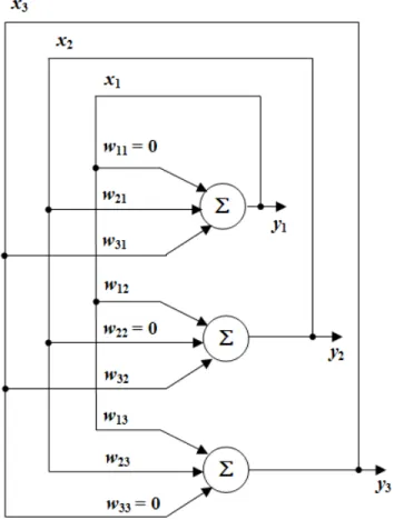
Figure 3-1 An example of an architecture of a Hopfield neural network consisting of 3 neurons (adapted from Haykin, 1999). ... 40
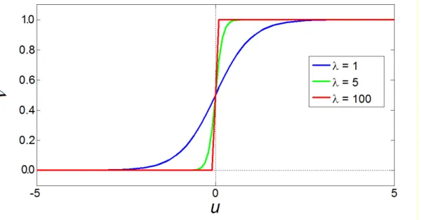
Figure 3-2 Hyperbolic tangent “tanh” function with different values of gain, = 1, = 5, and ... 42
Figure 3-3 A 2×2 pixels coarse spatial resolution image and representation of input neurons arrangement for the HNN derived from the sub-dividing pixels of the coarse spatial resolution image (adapted from Tatem et al., 2001a). ... 44
Figure 3-4 Multi-class constraint (a) an image showing five different types of classes including background, (b) Each class can be decomposed and assigned into four binary images, and (c) an arrangement of binary image of each band image creating a 3-dimensional matrix. ... 51
Figure 3-5 Location of Granada, Spain. ... 55
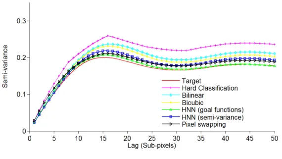
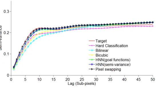
Figure 3-6 Original images of different spatial pattern of olive farms. (a) Sparsely populated, (b) densely populated, (c) globally heterogeneous, and (d) inter-grade. The size of each image is 256×256 pixels. ... 59
Figure 3-7 Degraded images from the original images in Figure 3.6. The size of each image is 32×32 pixels. ... 59
Figure 3-8 Target images. ... 59
Figure 3-9 Estimation results of hard classification technique. ... 60
Figure 3-10 Harden classification of bilinear interpolation technique. ... 60
Figure 3-12 Estimation results of HNN technique that used goal functions. ... 61 Figure 3-13 Estimation results of HNN technique that used semi-variance. ... 61 Figure 3-14 Estimation results of pixel swapping technique. ... 61 Figure 3-15 Variogram of different land cover estimation techniques for the sparsely populated land cover pattern. ... 64 Figure 3-16 Variogram of various land cover estimation techniques on a densely populated land cover pattern. ... 65 Figure 3-17 Variogram of various land cover estimation techniques on a heterogeneous land cover pattern. ... 66 Figure 3-18 Variogram of various land cover estimation techniques on an inter-grade land cover pattern. ... 67 Figure 3-19 „Mismatch classification‟ of using HNN that used semi-variance with different prior information. (a) Coarse spatial resolution of heterogeneous cover, (b) a priori knowledge from finer spatial resolution of densely populated land cover pattern, and (c) result of HNN that used semi-variance for super-resolution mapping. ... 69 Figure 4-1 Two white land cover patches on black land cover background. ... 76 Figure 4-2 Two white land cover patches overlaid with coarse spatial resolution grid image. The size of the patch A is larger than a coarse pixel while the size of the patch B is smaller. ... 76 Figure 4-3 Degradation of the image in Figure 4.1 by spatial aggregation into a coarse spatial resolution image... 76 Figure 4-4 Super-resolution mapping of land cover using the standard HNN. (a) A coarse spatial resolution with 4 white pure pixels, 4 black pure pixels and 1 mixed pixel. The soft classification value in the mixed pixel is 0.5. (b) Decomposition of coarse pixel into 8×8 sub-pixels with initial random allocation of white and black sub-pixels in the mixed pixel. (c) Estimation of land cover represented from HNN showing the boundary between two land cover classes (white and black) crossing inside the mixed pixel. ... 80 Figure 4-5 Super-resolution mapping of land cover using the standard HNN. (a) A coarse spatial resolution with 4 white pure pixels, 4 black pure pixels and 1 mixed pixel. The soft classification value in the mixed pixel is 0.2. (b) Decomposition of coarse pixel into 8×8 sub-pixels with initial random allocation of white and black sub-pixels in the mixed pixel. (c) Estimation of land cover represented from HNN showing the boundary between two land cover classes (white and black) crossing inside the mixed pixel. ... 80
Figure 4-6 Super-resolution mapping of land cover using the standard HNN. (a) A coarse spatial resolution with 8 black pure pixels and 1 mixed pixel. The value of soft classification in the mixed pixel is 0.5. (b) Decomposition of coarse pixel into 8×8 sub-pixels with initial random allocation of white and black sub-sub-pixels in the mixed pixel. (c) Estimation of land cover represented from HNN showing a land cover that smaller than the size of the mixed pixel... 82 Figure 4-7 Super-resolution mapping of land cover using the standard HNN. (a) A coarse spatial resolution with 8 black pure pixels and 1 mixed pixel. The soft classification value in the mixed pixel is 0.2. (b) Decomposition of coarse pixel into 8×8 sub-pixels with initial random allocation of white and black sub-pixels in the mixed pixel. (c) Estimation of land cover derived from HNN showing that no land cover could be represented... 82 Figure 4-8 Relationship of the input and output of HNN in representing large land cover patches using HNN(E), HNN(G), and HNN(A). The number of iteration for each HNN was 10,000. ... 88 Figure 4-9 Relationship of output and input of the HNN(E) using different numbers of iteration on a large land cover patch. ... 90 Figure 4-10 Relationship of output and input of the HNN(G) using different numbers of iteration on a large land cover patch. ... 91 Figure 4-11 Relationship of output and input of the HNN(A) using different numbers of iteration on a large land cover patch. ... 92 Figure 4-12 Relationship of the response of input and output of HNN in representing small land cover patches using HNN(E), HNN(G), and HNN(A). The number of iteration for each HNN was 10,000... 96 Figure 4-13 Relationship of output and input of the HNN(E) using different numbers of iteration on a small land cover patch... 98 Figure 4-14 Relationship of output and input of the HNN(G) using different numbers of iteration on a small land cover patch... 99 Figure 4-15 Relationship of output and input of the HNN(A) using different numbers of iteration on a small land cover patch... 100 Figure 4-16 The outputs of HNN(A) with the weight settings were k1k2 0.1,
1.0 P
k . (a) Input from soft classification. The value of soft classification = 0.20. (b) Random initialization. Results after (c) 1000 iterations, (d) 2000 iterations, (e) 5000
iterations, (f) 10,000 iterations, (g) 15,000 iterations, and (h) final mapping. (i) Intensity scale used to represent the soft classification value in a mixed pixel. ... 103 Figure 4-17 Relationship between output and input of the HNN to represent small land cover patches with the weight of the goal function was set constant at 1.0, and the weights for the area proportion constraint varied. The number for the iteration was set to 10,000. ... 105 Figure 4-18 Relationship between output and input of the HNN to represent small land cover patches with the weight for the area proportion constraint was set constant at 1.0, and the weights for the goal functions varied. The number for the iteration was set to 10,000. ... 106 Figure 4-19 Relationship of the response of input and output of pixel swapping in representing large land cover patches. ... 109 Figure 4-20 Relationship of the response of input and output of pixel swapping in representing small land cover patches. ... 111 Figure 4-21 Representation of land cover patches concerning on a problem of boundary of the patches at a sub-pixel scale. (a) Original fine spatial resolution image. (b) Degraded image. Super-resolution mapping using (c) HNN(E), (d) HNN(A), (e) PS(1), and (f) PS(5). ... 114 Figure 4-22 Representation of land cover patches concerning on a problem of a linear patch at sub-pixel scale. (a) Original fine spatial resolution image. (b) Degraded image. Super-resolution mapping using (c) HNN(E), (d) HNN(A), (e) PS(1), and (f) PS(5). . 115 Figure 4-23 Representation of land cover patches concerning on a problem of small patches at a sub-pixel scale. (a) Original fine spatial resolution image. (b) Degraded image. Super-resolution mapping using (c) HNN(E), (d) HNN(A), (e) PS(1), and (f) PS(5). ... 116 Figure 5-1 Illustration of the effect of mis-location of small patches in land cover mapping. (a) Reference image. (b) Land cover mapping with only a large patch represented. (c) Land cover mapping with a large patch and only four small patches represented. The locations of the small patches are slightly offset from the location in the reference image. ... 126 Figure 5-2 Spatial correspondences between patches in (a) Figure 5.1b with the reference image, and (b) Figure 5.1c with the reference image. ... 126
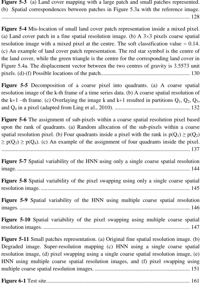
Figure 5-3 (a) Land cover mapping with a large patch and small patches represented. (b) Spatial correspondences between patches in Figure 5.3a with the reference image. ... 128 Figure 5-4 Mis-location of small land cover patch representation inside a mixed pixel. (a) Land cover patch in a fine spatial resolution image. (b) A 3×3 pixels coarse spatial resolution image with a mixed pixel at the centre. The soft classification value = 0.14. (c) An example of land cover patch representation. The red star symbol is the centre of the land cover, while the green triangle is the centre for the corresponding land cover in Figure 5.4a. The displacement vector between the two centres of gravity is 3.5573 unit pixels. (d)-(f) Possible locations of the patch... 130 Figure 5-5 Decomposition of a coarse pixel into quadrants. (a) A coarse spatial resolution image of the k-th frame of a time series data. (b) A coarse spatial resolution of the k+1 –th frame. (c) Overlaying the image k and k+1 resulted in partitions Q1, Q2, Q3,
and Q4 in a pixel (adapted from Ling et al., 2010). ... 132
Figure 5-6 The assignment of sub-pixels within a coarse spatial resolution pixel based upon the rank of quadrants. (a) Random allocation of the sub-pixels within a coarse spatial resolution pixel. (b) Four quadrants inside a pixel with the rank is p(Q1) ≥ p(Q2) ≥ p(Q3) ≥ p(Q4). (c) An example of the assignment of four quadrants inside the pixel.
... 137 Figure 5-7 Spatial variability of the HNN using only a single coarse spatial resolution image. ... 144 Figure 5-8 Spatial variability of the pixel swapping using only a single coarse spatial resolution image. ... 145 Figure 5-9 Spatial variability of the HNN using multiple coarse spatial resolution images. ... 146 Figure 5-10 Spatial variability of the pixel swapping using multiple coarse spatial resolution images. ... 147 Figure 5-11 Small patches representation. (a) Original fine spatial resolution image. (b) Degraded image. Super-resolution mapping (c) HNN using a single coarse spatial resolution image, (d) pixel swapping using a single coarse spatial resolution image, (e) HNN using multiple coarse spatial resolution images, and (f) pixel swapping using multiple coarse spatial resolution images. ... 151 Figure 6-1 Test site ... 161
Figure 6-2 Datasets (a) one of the MODIS 250 m near IR images acquired on 5 July 2002 and (b) Landsat ETM+ 30 m near IR image taken on 10 July 2002 that was used as
ground data. ... 161
Figure 6-3 Temporal coverage of a time-series daily MODIS 250 m. A MODIS image acquired on 5 July 2002 was used as a reference image for a time series image registration. Landsat image acquired on 10 July 2002 was used as a ground data as a means to set the orientation of the MODIS image correctly. ... 162
Figure 6-4 Ground data. ... 171
Figure 6-5 Hard classifier. ... 171
Figure 6-6 Proportional image derived from fuzzy c-means soft classification. ... 171
Figure 6-7 Application of a MODIS image into (a) PS(1) and (b) PS(5). ... 172
Figure 6-8 Application of a MODIS image into (a) PS(1) and (b) PS(5). Results of both techniques were filtered with a 3×3 median filter. ... 172
Figure 6-9 Application of a MODIS image into (a) PS(1) and (b) PS(5). Results of both techniques were filtered with a 5×5 median filter. ... 173
Figure 6-10 Application of a MODIS image into (a) HNN(E) and (b) HNN(A). ... 173
Figure 6-11 Application of a MODIS image into HNN2 approach... 174
Figure 6-12 Proportional image derived from a fusion of proportional images of a MODIS time series. ... 183
Figure 6-13 Application of a fused time series MODIS images into (a) PS(1) and (b) PS(5). ... 183
Figure 6-14 Application of a fused time series MODIS images into (a) PS(1) and (b) PS(5). Results of both techniques were filtered with a 5×5 median filter. ... 184
Figure 6-15 Application of a fused time series MODIS images into (a) HNN(E) and (b) HNN(A)... 184
Figure 6-16 Application of a fused time series MODIS images into HNN2 approach. 185 Figure 6-17 Texture values for different land cover mapping techniques as a function of angle for homogeneity. Low homogeneity indicates high number of small lakes presented in an image, such as image in the ground data. ... 192
Figure 6-18 Texture values for different land cover mapping techniques as a function of angle for contrast. High contrast indicates high number of small lakes presented in an image, such as image in the ground data... 192 Figure 6-19 Texture values for different land cover mapping techniques as a function of angle for inverse difference moment (IDM). High IDM indicates that more large lakes are presented in an image than small lakes. The high number of small lakes in the ground data decreases the IDM value as in the ground data. ... 193 Figure 6-20 Texture values for different land cover mapping techniques as a function of angle for entropy. High entropy indicates that the complexity of the spatial distribution of lakes is high in an image, such as image in the ground data. ... 193 Figure 6-21 Selected lakes used for object based analysis... 196 Figure 6-22 Boundary fitting for different techniques on lake 25. The red line indicates the boundary of the lake from the ground data image, and the blue line indicates the boundary of the represented lake. ... 203 Figure 6-23 Positional error along the boundary of lake 25. ... 204 Figure 7-1 Illustration of the initial spatial arrangement of hard classifier at a sub-pixel scale. (a) Several mixed pixels with different proportion of black and white classes. Values at the bottom indicate the proportion of the white class. (b) Initial spatial arrangement using random technique. (c) Initial spatial arrangement using halftoning technique. ... 212 Figure 7-2 The Landsat ETM+ data of the test site. (a) near-infrared waveband image and (b) binary land cover map derived from hard classification. ... 214 Figure 7-3 A simulated image with a spatial resolution of 240 m derived by spatial degradation of the Landsat ETM+ imagery. ... 214 Figure 7-4 The MODIS images ... 215 Figure 7-5 Diagram of the proposed new super-resolution mapping technique ... 217 Figure 7-6 Soft classification on (a) a single coarse spatial resolution image, (b) a fusion of multiple coarse spatial resolution images. ... 219 Figure 7-7 Initialization of binary class proportions on a sub-pixel scale using (a) random dot pattern, (b) dispersed halftoning dot pattern. Correspondence Fourier of (c) random dot pattern, (d) halftoning dot pattern. ... 221
Figure 7-8 Image reconstruction using 2D multiple notch filter (a) a 2D multiple notch filter, (b) result of the filter derived from Figure 6b. ... 224 Figure 7-9 An illustration of an iterative morphological thinning filter considers area estimation from soft classification of pixels enclosed by the delineation of boundary lines to be used as a constraint while shrinking the lake... 227 Figure 7-10 Results of the simulated coarse spatial resolution imagery. (a) the hard classification derived from a MODIS image acquired on 7 July 2002, (b) soft classification of the MODIS image, and (c) output from bilinear interpolation, (d) output from bicubic interpolation, (e) output from HNN, and (f) output from the super-resolution mapping using the halftoning concept. ... 233 Figure 7-11 Results of the real MODIS data. (a) the hard classification derived from a MODIS image acquired on 7 July 2002, (b) soft classification of the MODIS image, and (c) output from bilinear interpolation, (d) output from bicubic interpolation, (e) output from HNN, and (f) output from the super-resolution mapping using the halftoning concept. ... 234
List of tables
Table 3-1 Thematic accuracy comparison between different land cover mapping classification techniques for a sparsely populated land cover pattern ... 62 Table 3-2 Thematic accuracy comparison between different land cover mapping classification techniques for a densely populated land cover pattern ... 62 Table 3-3 Thematic accuracy comparison between different land cover mapping classification techniques for a globally heterogeneous land cover pattern ... 63 Table 3-4 Thematic accuracy comparison between different land cover mapping classification techniques for an inter-grade land cover pattern ... 63 Table 3-5 SSE for variogram of different land cover estimation techniques applied on a sparsely populated land cover pattern. ... 64 Table 3-6 SSE for variogram of different super-resolution mapping methods applied on a densely populated land cover pattern. ... 65 Table 3-7 SSE for variogram of different super-resolution mapping methods applied on a heterogeneous land cover pattern. ... 66 Table 3-8 SSE for variogram of different super-resolution mapping methods applied on an inter-grade land cover pattern... 67 Table 4-1 Average ratio of the output and input of the HNN(E) as a function of iteration on the representation of a large land cover patch from 20 coarse spatial resolution images. ... 90 Table 4-2 Average ratio of the output and input of the HNN(G) as a function of iteration on the representation of a large land cover patch from 20 coarse spatial resolution images. ... 91 Table 4-3 Average ratio of the output and input of the HNN(A) as a function of iteration on the representation of a large land cover patch from 20 coarse spatial resolution images. ... 92 Table 4-4 Average ratio of the output and input of the HNN(E) as a function of iteration on the representation of a small land cover patch from 20 coarse spatial resolution images. ... 98
Table 4-5 Average ratio of the output and input of the HNN(G) as a function of iteration on the representation of a small land cover patch from 20 coarse spatial resolution
images. ... 99
Table 4-6 Average ratio of the output and input of the HNN(A) as a function of iteration on the representation of a small land cover patch from 20 coarse spatial resolution images. ... 100
Table 4-7 Average ratio of the output and input of the HNN as a function of varying the weight of the area proportion constrain and setting the weight of the goal functions constant at 1.0... 105
Table 4-8 Average ratio of the output and input of the HNN as a function of varying the weights of the goal functions and setting the weight of the area proportion constraint constant at 1.0... 106
Table 4-9 Average ratio of the output and input of the pixel swapping as a function of different number of the neighbours on the representation of a large land cover patch from 20 coarse spatial resolution images. ... 109
Table 4-10 Average ratio of the output and input of the pixel swapping as a function of different number of the neighbours on the representation of a small land cover patch from 20 coarse spatial resolution images. ... 111
Table 4-11 Area measurement on patches (unit sub-pixels) ... 117
Table 4-12 Perimeter measurement on patches (unit sub-pixels) ... 117
Table 4-13 Positional accuracy of the boundary of the land cover patches (unit sub-pixels) ... 117
Table 4-14 Number of patches. ... 118
Table 5-1 Confusion matrix for land cover mapping in Figure 5.1b ... 127
Table 5-2 Confusion matrix for land cover mapping in Figure 5.1c ... 127
Table 5-3 Confusion matrix for land cover mapping in Figure 5.3a ... 128
Table 5-4 Statistics of the spatial variability of the HNN using only a single coarse spatial resolution image. Mean and variance were measured from 10 displacements of a patch in every increment of soft classification value in a mixed pixel. ... 144 Table 5-5 Statistics of the spatial variability of the pixel swapping using only a single coarse spatial resolution image. Mean and variance were measured from 10
displacements of a patch in every increment of soft classification value in a mixed pixel. ... 145 Table 5-6 Statistics of the spatial variability of the HNN using multiple coarse spatial resolution images. Mean and variance were measured from 10 displacements of a patch in every increment of soft classification value in a mixed pixel. ... 146 Table 5-7 Statistics of the spatial variability of the pixel swapping using multiple coarse spatial resolution images. Mean and variance were measured from 10 displacements of a patch in every increment of soft classification value in a mixed pixel. ... 147 Table 5-8 Confusion matrix for land cover mapping represented by HNN using a single coarse spatial resolution image. ... 152 Table 5-9 Confusion matrix for land cover mapping by pixel swapping using a single coarse spatial resolution image. ... 152 Table 5-10 Confusion matrix for land cover mapping represented by HNN using a time series coarse spatial resolution images. ... 152 Table 5-11 Confusion matrix for land cover mapping by pixel swapping using a time series coarse spatial resolution images. ... 153 Table 6-1 Landsat 7 ETM+ bands ... 160 Table 6-2 Relative translations at sub-pixel scales between a reference MODIS image acquired on 5 July 2002 and the rest of the images in the time series daily MODIS images. ... 165 Table 6-3 Notations for different super-resolution mapping techniques... 169 Table 6-4 Confusion matrix for hard classifier applied on a MODIS image ... 178 Table 6-5 Confusion matrix for PS(1) without median filter applied on a MODIS image ... 178 Table 6-6 Confusion matrix for PS(1) with a 3×3 median filter applied on a MODIS image ... 178 Table 6-7 Confusion matrix for PS(1) with a 5×5 median filter applied on a MODIS image ... 179 Table 6-8 Confusion matrix for PS(5) without median filter applied on a MODIS image ... 179
Table 6-9 Confusion matrix for PS(5) with a 3×3 median filter applied on a MODIS image ... 179 Table 6-10 Confusion matrix for PS(5) with a 5×5 median filter applied on a MODIS image ... 180 Table 6-11 Confusion matrix for HNN(E) applied on a MODIS image ... 180 Table 6-12 Confusion matrix for HNN(A) applied on a MODIS image ... 180 Table 6-13 Confusion matrix for HNN2 applied on a MODIS image ... 181
Table 6-14 Confusion matrix for PS(1) with a 5×5 median filter applied on a fused time series MODIS images ... 186 Table 6-15 Confusion matrix for PS(5) with a 5×5 median filter applied on a fused time series MODIS images ... 186 Table 6-16 Confusion matrix for HNN(E) applied on a fused time series MODIS images ... 186 Table 6-17 Confusion matrix for HNN(A) applied on a fused time series MODIS images ... 187 Table 6-18 Confusion matrix for HNN2 applied on a fused time series MODIS images
... 187 Table 6-19 Comparison of landscape parameters and texture variables from various super-resolution mapping techniques. Results shown in bold indicate that the prediction is the closest to the ground data. ... 191 Table 6-20 Comparison of area, (km2). Bold and underlined results indicate predictions closest to the ground data. ... 198 Table 6-21 Comparison of Perimeter, (m). Bold and underlined results indicate predictions closest to the ground data. ... 199 Table 6-22 Comparison of compactness. Bold and underlined results indicate predictions closest to the ground data. ... 200 Table 6-23 Comparison of RMSE on boundary fitting (m). Bold and underlined results indicate predictions closest to the ground data. ... 207 Table 7-1 Lake characterisations of area and perimeter from the simulated coarse spatial resolution imagery; the difference from the ground reference data is shown in brackets (positive values indicate over-estimation). ... 235
Table 7-2 Lake characterisations of length and compactness from the simulated coarse spatial resolution imagery; the difference from the ground reference data is shown in brackets (positive values indicate over-estimation). ... 236 Table 7-3 Lake characterisations of area and perimeter from the MODIS imagery; the difference from the ground reference data is shown in brackets (positive values indicate over-estimation). ... 237 Table 7-4 Lake characterisations of length and compactness from the MODIS imagery; the difference from the ground reference data is shown in brackets (positive values indicate over-estimation). ... 238
List of abbreviations and acronyms
ART Adaptive Resonance Theory ARTMAP Adaptive Resonance Theory MAP
AVHRR Advanced Very High Resolution Radiometer DN Digital Number
ETM+ Enhanced Thematic Mapper Plus GLCM Gray-Level Co-occurrence Matrix HNN Hopfield Neural Network
HRG High Resolution Geometry IBP Iterative Back-Projection IDM Inverse Difference Moment LIDAR Light Detection and Ranging MAP Maximum A Posteriori
MERIS Medium Resolution Imaging Spectrometer ML Maximum Likelihood
MLP Multi-Layer Perceptron
MODIS Moderate Resolution Imaging Spectroradiometer MRF Markov Random Field
MS Multispectral PAN Panchromatic
POCS Projection Onto Convex Sets RMSE Root Mean Squared Error RSR Relative Spectral Response RVM Relevance Vector Machine
SPOT Système Probatoire d'Observation de la Terre SVM Support Vector Machine
1.
Introduction
1.1. Overview
The mosaic of land cover types that occur on the Earth‟s surface is a key variable in a
range of environmental systems (Falcucci et al., 2007; Lucas et al., 2007). For example, the landscape mosaic impacts on a large and diverse array of issues that include the aesthetic appeal of a region, its biodiversity and its climate. Land cover and land cover change are, for example, critical variables affecting ecological systems (Ruelland et al., 2010; Brink and Eva, 2009; Serra et al., 2008). Information on land cover is, therefore, required in a range of studies, with some, especially those associated with landscape ecology, requiring information on the nature of landscape patches (e.g. their size, shape etc). Remote sensing has considerable potential as a source of information on land cover at a range of spatial and temporal scales (Boyd and Foody, 2011; Addink et al., 2010; Buermann et al., 2008).
Although remote sensing is widely used as a source of land cover information for ecological studies (Newton et al., 2009) there are many factors that limit the accuracy of derived land cover information (Foody, 2002). These include the classification algorithm and pre-processing methods used as well as the temporal and
spatial resolution of the data. The latter is the key focus of attention in this thesis, with the accuracy may be characterised known to be a function of the spatial resolution of the imagery and minimum mapping unit used (Saura, 2002).
The land cover mosaic of a region typically comprises a set of patches of relatively homogenous cover that can be considered as objects within a remotely sensed image. To characterise objects accurately it is important that the image spatial resolution or pixel size is smaller than the typical size of the objects (Woodcock and Strahler, 1987). This may require use of imagery with a fine spatial resolution.
Spatial resolution can be treated as a variable in sensor selection for a project and
needs to be determined in relation to the project‟s specific goals and sensing systems
properties (Warner et al., 2009). Imagery with a fine spatial resolution have been acquired from space for many years, notably through military systems such as the US Keyhole (KH) or CORONA series of satellites from the late 1950s to early 1970s (McDonald, 1995; Toutin, 2009). A large number of fine and very fine spatial resolution systems have also been developed in recent years. There are ~36 satellite systems in orbit or scheduled for launch that are able to provide imagery with a spatial resolution of < 3 m (Toutin, 2009). These systems have revolutionised aspects of remote sensing with, for example, the new fine spatial resolution sensing systems now allow mapping at scales ~1:5,000 from ~0.6 m resolution QuickBird imagery (Topan et al., 2009). The main drawback to the use of these systems is the cost of the imagery (Toutin, 2009). For example, Toutin (2009) suggests that even relatively basic image products from fine spatial resolution sensors costs ~US$20 km-2 and more highly processed products may be several times more expensive still. Imagery from slightly coarser spatial resolution
systems such as Système Probatoire d'Observation de la Terre High Resolution Geometry (SPOT HRG) (spatial resolution ~4-10 m) costs only ~US$3-5 km-2. Moreover, the extent of the imagery from SPOT HRG is much larger than from IKONOS; some 36 IKONOS images would be required to cover the same area as a single SPOT HRG image (Toutin, 2009). There have also been many major developments in medium-coarse spatial resolution systems (Goward et al., 2009; Justice and Tucker 2009) and, critically, these can provide inexpensive imagery of relatively large areas. Projects may often be constrained to use such relatively coarse spatial resolution imagery for pragmatic reasons.
Often the spatial resolution of a remote sensor is too coarse for the intended application and inappropriate for optimal mapping. Land cover data derived in such circumstances should be used with care. The errors and uncertainties in land cover derived from remote sensing may sometimes go unrecognised and can greatly impact on the characterisation of landscapes (Shao and Wu, 2008). One major problem arising from the use of coarse spatial resolution imagery is mixed pixels (Fisher, 1997). A mixed pixel contains more than one land cover class and cannot be appropriately
represented by the standard „hard‟ allocation process used in conventional image
classification algorithms (one pixel – one class). Unfortunately mixed pixels may be common and the proportion of mixed pixels tends to increase with an increase in pixel size, with mixed pixels typically vastly dominating imagery acquired at a coarse spatial resolution.
There are four common land cover mosaic scenarios that could cause mixed pixel (Fisher, 1997) (Figure 1.1). They are: (1) sub-pixel sized patches: the size of a land
cover class captured within a pixel is smaller than the size of the pixel, thus allowing a space within the pixel for another land cover class; (2) boundary pixel: the size of two or more land cover classes on the ground may be bigger than the size of the pixel, but parts of their boundaries lie in a single pixel; (3) inter-grade: a pixel allocates a space for a transition from a cluster of one class to a cluster of another class; and (4) linear sub-pixel: the length of a land cover class may be longer than a pixel but its width is thinner, and the land cover class runs through a pixel.
A popular adaptation of the standard approach to land cover mapping that allows for mixed pixels is the use of a fuzzy or soft classification (Foody, 1996). The latter allows a pixel to have multiple and partial class membership and outputs typically a set
of fraction images, each showing the proportion of the pixel‟s area that is covered by a
specific land cover class. Although attractive in reducing the mixed pixel problems a concern is that the soft classification does not show the spatial distribution of the sub-pixel class fractions limiting its value as a source of information on landscape objects (Atkinson, 1997).
An alternative way to address the mixed pixel problem is to adopt some form of spatial resolution enhancement technique to increase the spatial resolution of imagery (i.e. to reduce the effective pixel size). For example, methods based on image sharpening, especially if the sensor operates at more than one spatial resolution (Mather, 2004) or super-resolution analyses (Tatem et al., 2001a; Lu and Inamura, 2003; Ling et al., 2010). The aim of the latter is to effectively decrease the pixel size, allowing
(a) (b)
(c) (d)
Figure 1-1 Four causes of mixed pixel: (a) sub-pixel sized patches, (b) boundary pixel, (c) inter-grade, and (d) linear sub-pixel (adapted from Fisher, 1997).
interpretation of sub-pixel scale features. Approaches adopted are typically based on either super-resolution restitution or super-resolution mapping (Ling et al., 2010) and their use can add value to relatively inexpensive image data sets.
A variety of super-resolution mapping techniques have been used in remote sensing and related research (Tatem et al., 2001a; Verhoeye and De Wulf, 2002; Mertens et al., 2003, 2004; Foody et al., 2005; Farsiu et al., 2006). Typically these techniques have been applied with a single coarse spatial resolution image as their input. Although the technique may be used to derive a land cover map at a finer spatial scale than the input imagery, there are many concerns with their use. One is that small isolated patches of a land cover class are often not represented or only inaccurately (Kasetkasem et al., 2005). Additionally the use of a single input image may limit the accuracy of land cover representation and the use of multiple coarse resolution images may offer an ability to enhanced accuracy. Given that coarse spatial resolution systems often have a relatively fine temporal resolution it may be possible to derive multiple images of the same site over a short period of time as input to a super-resolution analysis. The images in the time series may differ in subtle ways, with the location of pixels varying slightly due to, for example, minor orbital translations of remote sensing satellites. The slight differences between images can be exploited by combining a time-series coarse spatial resolution images into an integrated image which may contain more information than a single coarse spatial resolution image (Packalen et al., 2006). Exploiting the fine temporal resolution that is characteristic of many coarse spatial resolution remote sensing systems (Ling et al., 2010) may, therefore, facilitate super-resolution analyses.
1.2. Objectives
The work reported in this thesis focuses on the representation of small land cover patches. As illustrated graphically in Figure 1.1 that there are four cases that cause the mixed pixel problem. Many of the current super-resolution mapping techniques are able
to solve the „boundary pixel‟, „inter-grade‟ (e.g. Tatem et al., 2001a), and „linear sub
-pixel‟ (Thornton et al., 2007) cases. However, there is lack of comprehensive research
study on the „sub-pixel‟ sized patches case (Zhan et al., 2002). The attention of this
thesis is on the „sub-pixel‟ case, which the size of the land cover patches is smaller than a pixel.
The key thrust of this thesis is on the derivation of accurate land cover map using super-resolution mapping techniques. In particular, the thesis focuses on two key issues. First the accuracy with which the area of small patches is estimated. Second the accuracy with which the small patches are located geographically.
The main objective of this thesis is to improve current super-resolution mapping techniques as well as to develop a novel super-resolution mapping techniques in order to solve the two challenges listed above.
The improved or new super-resolution mapping techniques should be able to represent small land cover patches accurately. The latter will be demonstrated using a range of measures of accuracy (e.g. site specific, landscape parameter accuracy, object based accuracy, and positional accuracy) and compared with current super-resolution mapping techniques. The improved or new super-resolution mapping techniques should
help to keep the cost of acquiring remotely sensed images as low as possible. This would increase the value for the coarse spatial resolution imagery.
In order to achieve the objectives listed above, experiments reported in this thesis were undertaken using synthetic image and real image (e.g. MODIS 250 m image and a fusion of a time series MODIS 250 m images as well as Landsat ETM+ 30 m is used as a ground data for benchmark comparison). Attention is focused on a real-world application: the mapping of high latitude lakes (Smith et al., 2005). Landscape mosaic that is made up of lakes of varying shape, size and spatial configuration is used as it may contain all the four cases of the mixed pixels, which is highlighted in Figure 1.1, although the attention of the thesis is on the „sub-pixel‟ sized patches case.
1.3. Thesis structure
This thesis is organised into eight chapters, including the present chapter. A brief summary of the other chapters is provided below.
Chapter 2 provides an overview of resolution techniques including super-resolution restitution (reconstruction) and super-super-resolution mapping; the differences between these two concepts will be addressed. A brief overview on soft classification techniques is included as they become pre-requisite for many super-resolution mapping techniques. This chapter also provides an overview of different assessment methods for evaluating results of super-resolution mapping techniques such as confusion matrix for site specific accuracy, landscape indices for spatial pattern analysis, object based
analyses for shape characterization and positional accuracy to determine the fitting of the boundary line between land cover patches.
Chapter 3 details the fundamental principles of two standard super-resolution mapping techniques based on a Hopfield neural network (HNN) and pixel swapping techniques. A section that details the fundamental principle of a fuzzy c-means technique will be presented as it can be used to derive soft classification from mixed pixels, which will be used as input for both of the super-resolution mapping techniques. Remote sensing images containing various spatial patterns are used. Sets of coarse spatial pattern images are derived by spatially aggregating the original images. Analyses on these techniques are focused on the site specific accuracy and spatial pattern variogram. This chapter serves as a pilot chapter, which aim to explore the standard techniques. Results of this chapter confirmed the advantages and limitations for each technique and help define the research direction.
Chapter 4 highlights the limitations of the standard HNN and pixel swapping in representing small land cover patches. The parameter setting of the HNN and pixel swapping are evaluated in a series of experiments using a single coarse spatial resolution image. In these experiments, the optimum values of the parameters that can represent small land cover patches are obtained.
Chapter 5 highlights the spatial variability of patch location from the use of the standard HNN and pixel swapping algorithms. It is demonstrated in this chapter that high spatial variability may lead to decreasing accuracy of the site specific assessment.
Using multiple sub-pixels shifted image observations, the spatial variability can be reduced, which lead to accurate localization of small land cover patches.
Chapter 6 outlines an enhanced HNN and pixel swapping methods and demonstrates their application in representing a landscape mosaic that is made up of lakes of varying shape and size from MODIS 250 m images. A fusion of time series MODIS imagery is also presented. A series of assessment such as site specific accuracy, landscape indices, object based characterization and positional accuracy are implemented in order to evaluate the representation of the lakes.
Chapter 7 presents a novel super-resolution mapping technique based on halftoning concept. This new technique provides an alternative to the current super-resolution mapping techniques in which the spatial frequency of the initial distribution of hard classifier at a sub-pixel scale of mixed pixels could be exploited.
Finally in Chapter 8, the conclusions of the research in this thesis are gathered and recommendations for future works are presented.
2.
Background
This chapter reviews the background to super-resolution mapping to gain an understanding required for this thesis. Subjects reviewed include the super-resolution restitution, super-resolution mapping, soft classification, as well as accuracy assessment methods.
2.1. Super-resolution restitution
Super-resolution restitution or reconstruction is a technique to construct a fine spatial resolution image from a multiple coarse spatial resolution images by recovering the high-frequency component of image content (Yang and Huang, 2011). Super-resolution restitution consists of image registration from a set of coarse spatial resolution images and image restitution (reconstruction). During the restitution process, this technique combines non-redundant information contained in the coarse spatial resolution images and generate a fine spatial resolution image. This section reviews different approaches of the super-resolution restitution.
2.1.1. Frequency domain approach
The super-resolution concept was first introduced by Tsai and Huang (1984). Given several coarse spatial resolution images, a fine spatial resolution image is constructed in the frequency domain. The frequency domain is obtained through the transformation from the spatial domain using the Fourier transform. Their approach is based on the principles of the shifting property of the Fourier transform. The aliasing relationship between continuous Fourier transform of the original image and the discrete Fourier transform of the observed coarse spatial resolution images is considered. This technique assumes that the original fine spatial resolution is band-limited. It was assumed that the observations of the coarse spatial resolution images sequence are free from degradation and noise.
Kim et al. (1990) restored a fine spatial resolution image from noisy and blurred images. They used a recursive algorithm made up from a combination of two steps of filtering and reconstruction in the frequency domain. The filtering operation is used in the image registration to compensate the degradation and noise, and the reconstruction operation estimates the fine spatial resolution image. Every coarse spatial resolution observation image is assumed to have similar blur and noise characteristics. Later, Kim and Su (1993) made an improvement in this method by considering different amounts of blur for each coarse spatial resolution image. Tikhonov regularization (Tikhonov and Arsenin, 1977) is used to obtain a solution for inconsistent set of linear equations.
The major advantage of this approach is the theoretical simplicity in term of describing the relationship between coarse images and fine image in the frequency
domain. However, every coarse image is assumed to be affected by a translational motion and a linear space invariant blur. This is seemed as a limitation of the frequency domain approaches to handle various situations. Moreover, it is difficult to apply a priori knowledge in this domain because the data are uncorrelated in the frequency domain (Park et al., 2003).
2.1.2. Spatial domain approach
A method to reconstruct a finer spatial resolution image in the spatial domain was proposed by Stark and Oskui (1989) known as projection onto convex sets (POCS). The method is an extension of a convex projection theory used in computed tomography for one-dimensional signals (Oskui and Stark, 1988). The POCS method constructs a finer resolution image by scanning or rotating the image with respect to image-plane detector arrays. Prior information can be incorporated in this method to increase the quality of the image. This method considers the effect of noise in the data. This method requires iterative computation, thus slow convergence is one of its limitations. In addition, because POCS optimizes a purely constraint based objective, it does not converge to a unique solution (Park et al., 2003).
The concept of reconstruction of a 2-D object from its 1-D projection in computed tomography also inspired Irani and Peleg (1991) to reconstruct a fine spatial resolution image. The super-resolution problem is formulated as an Iterative Back-Projection (IBP) procedure. This method starts with an initial guess of a fine spatial resolution image. A set of coarse spatial resolution simulated images are created
corresponding to an observed coarse spatial resolution input image. The simulated images are created by shifting the pixels of the observed input image in the horizontal and vertical directions. The difference between the simulated images and the observed image is computed to improve the initial guess of a fine spatial resolution image. This algorithm projects the difference values backward and includes it while updating the desired fine spatial resolution image. This process is repeated iteratively to minimize the error function. For a single image, the super-resolution process, which is designed for sequences of images, is reduced to a problem of de-blurring an image. This technique converges quickly by fixing stable pixels. When a pixel has the same value or nearly the same value in two successive iterations, the pixel would not be considered in the next iteration, helping to accelerate the convergence process. Unlike the POCS method, the IBP procedure does not involve prior constraints. Both POCS and IBP methods are not restricted to have a specific motion characteristic. They are able to work with smooth motion, linear space variant blur, and non-homogeneous additive noise.
2.1.3. Motionless super-resolution
All the previous methods assume that there is small relative motion in the image sequences, however, Elad and Feuer (1997) demonstrated that motionless super-resolution reconstruction could be made possible from a sequence of coarse spatial resolution images which are spatially aggregated caused by a series of transformations such as geometrical warping, blurring, noisy. A hybrid algorithm is proposed from a combination of maximum likelihood (ML) estimator and the POCS algorithm. This
technique exploits the advantages of the simple ML estimator and the ability of the POCS to incorporate non-ellipsoids constraints. This technique, however, assumes a linear space variant blur, and an additive Gaussian noise.
2.1.4. Recognition based super-resolution
Baker and Kanade (2002) suggested incorporating super-resolution technique with other module in order to overcome several constraints in conventional super-resolution techniques, especially for a case of input image that is too coarse. Increasing the resolution of image containing human face could be implemented with a combination of Bayesian MAP super-resolution and a face recognition technique. This technique is known as recognition-based super-resolution or hallucination. The drawback of this algorithm is it only works with images containing a face. Results of this technique on image not containing faces showed an outline of a face, which has been hallucinated into the image even though there is no face in the input image.
2.1.5. Super-resolution restitution in remote sensing
Super resolution restitution techniques have also been applied in remote sensing applications to reconstruct a fine spatial resolution image from a set of coarse spatial observations. Examples of the application of the super-resolution restitution in remote sensing include Akgun et al. (2005), Merino and Nunez, (2007), Hu et al., (2009), and Shen et al. (2009).
2.2. Super-resolution mapping
Unlike the super-resolution restitution that only enhances the spatial resolution of imagery, super-resolution mapping is a land cover classification technique that produces thematic classifications at a sub-pixel scale (Atkinson, 2004). Soft classification may be used to estimate the class composition of image pixels but the spatial distribution of each class in these mixed pixels cannot be determined. Therefore, the attention of the super-resolution mapping is to estimate the location of the component of land cover classes within a pixel, with the proportion of the classes determined from a soft classification technique. This section first reviews soft classification techniques and then followed by a review of a variety of super-resolution mapping techniques.
2.2.1. Soft classification
The fundamental unit of a remotely sensed image is the pixel. The number of pixels in an image depends on the spatial resolution of a sensor. The pixel shows information on the spectral response of an area on the ground. The area presented in a pixel is determined by the sensor. A pixel may contain more than one thematic class. In such situation, the partitions of the thematic classes are mixed within a pixel (Fisher, 1997; Cracknell, 1998). The proportion of the mixed pixels depends on the spatial resolution of sensor and land cover mosaic on the ground (Foody 2005). The proportion of the mixed pixel increases with a coarsening of the spatial resolution and/or with increasing the fragmentation of the landscape presented in the image. Conventional hard classification method assumes that a pixel is pure, discrete and contains only one
thematic class, thus this method is not able to accurately classify mixed pixels. Therefore, soft classification methods which are able to perform classification at the sub-pixel level have been developed to un-mix the mixed pixel and to determine the composition of the pixel, which is not necessarily contain just one thematic class. This section reviews a variety of soft classification techniques, which have been used to estimate sub-pixel class composition within a mixed pixel.
2.2.1.1. Linear mixture model
An early method to estimate the sub-pixel class composition in a mixed pixel was proposed by Settle and Drake (1993) using a linear mixture model. They determined the relative proportion of ground cover components in a mixed pixel by assuming that the spectral response of the mixed pixel is a linear weighted sum of spectral responses of its component classes. The linear spectral mixture model offers simplicity and accurate sub-pixel estimation. However, the use of the least square error criterion in this method hinders the un-mixing analysis to solve problems involving outliers. Outlier is defined as a pixel with atypical value, which does not belong to any predefined class. Instead of
using a least square method, Rosin (2001) reduced the outliers‟ effect by using a least
median square (LMedS) method. Borel and Gerstl (1994) demonstrated that linear un-mixing model was not suitable for nonlinear mixture problem. As such, non-linear mixing models were proposed (Borel and Gerstl, 1994; Foody and Arora, 1997).
2.2.1.2. Maximum likelihood classification
The maximum likelihood (ML) classifier is a supervised statistical classification technique that is based on the Bayesian probability framework (Tso and Mather, 2009). The ML classifier calculates the probability of a pixel belonging to a predefined set of classes, and assigns a class to a pixel that has the highest posterior probability of membership. Although the classification of a pixel to one thematic class leads to the hard classification problem, the ML classifier can be adapted in the soft classification problem by assigning the procedure of the ML classifier at the sub-pixel level (Foody et al., 1992). The use of likelihood functions as estimators of mixing is valid if the classes of interest are high separable and distributions overlap only slightly (Schowengerdt, 1995).
2.2.1.3. Fuzzy c-means
The fuzzy c-means algorithm is an unsupervised data clustering technique in which a group of data can be subdivided into c clusters or classes. Every pixel in the dataset belongs to every cluster to a certain degree of membership rather than belonging completely into just one cluster. For example, a pixel that lies close to the centre of a cluster will have a higher degree of membership than another pixel which lies far away than the centre of the cluster. This method was developed by Dunn (1973) and improved by Bezdek (1981) and Bezdek et al., (1984). Fuzzy c-means starts by assigning pixels to classes randomly. Next, every pixel is given a membership degree for each class. Fuzzy partitioning is performed iteratively with the update of membership and centre of class.
The iteration aims to minimize an objective function that represents the distance from an
arbitrary pixel in an image to centre of a class weighted by the pixel‟s membership
grade.
Fuzzy c-means has been used in remote sensing to derive sub-pixel scale thematic information (Fisher and Pathirana, 1990; Foody, 1996; Atkinson et al. 1997; Bastin, 1997). Atkinson et al. (1997) reported that fuzzy c-means was more accurate than mixture modelling but less accurate when compared with artificial neural network. In estimating sub-pixel thematic information from remotely sensed images, (Foody, 1996; Atkinson et al. 1997; Bastin, 1997; Lucas et al. 2002) the fuzzy c-means has also been used in supervised mode. The accuracy of the fuzzy c-means is subject to a value of weighting parameter which must be carefully selected by user (Foody, 1996). Fuzzy c-means generally produces accurate class composition estimates when all classes have been defined and included in the training phase of the classification. However, the presence of untrained classes would degrade the estimation accuracy of the fuzzy c-means; therefore a counterpart of this technique, namely possibilistic c-means is used for robustness towards the untrained classes (Krishnapuram and Keller, 1993; Krishnapuram and Keller, 1996; Foody, 2000).
2.2.1.4. Feed-forward neural network
Neural network is a popular solution related to the classification problems because its ability to solve nonlinear mixture problems (Carpenter et al., 1999; Foody, 2001; Liu et al. 2004). Problems involving data classification in remote sensing have been solved
using a variety of feed-forward neural network such as multi-layer perceptron (MLP), radial basis function, and probabilistic neural network. Each of them is constructed from a fundamental unit of processing element or neuron, which is arranged in a layered network. The way the neuron is arranged in a network and the activation functions used differentiate all the three aforementioned models. Given enough training data and a priori knowledge, neural network can be an effective non-parameter solution.
Mixed pixels can be included in the feed-forward neural networks during the training stage. The trained networks can be used to predict the class membership properties for other pixels in the data set. In addition to the feed-forward neural networks, a neural network based on adaptive resonance theory (ART) has been used and known as ARTMAP. The ARTMAP learning is faster and more stable than ML classifier, MLP, or k-nearest neighbour techniques. Another advantage of the ARTMAP is that the learning process can be performed online for recognition and prediction tasks. A major drawback of neural network techniques is their lack of ability to explain physical system being modelled (Liang et al., 2008).
2.2.1.5. Support vector machine
Support vector machine (SVM) is a supervised classification and regression methods based on statistical learning theory (Vapnik, 1995). SVM is fundamentally a binary classifier, which treats input data as two sets of vector in an n-dimensional space. SVM constructs a separating hyper-plane in that space to maximize margin between the two data sets. Large margin decreases generalization error of the classifiers. Brown et al.
(2000) showed that a constrained least squares linear spectral mixture model is equivalent to a linear SVM. Linear SVM uses linear discrimination to separate classes which are linearly separable. Linear SVM is able to select support vectors automatically from a larger database and is more appropriate for empirical mixture modelling. The accuracy of the SVM classification is not dependent on large datasets in the training and a complete descri