Lehigh University
Lehigh Preserve
Theses and Dissertations
2018
Efficient Trust Region Methods for Nonconvex
Optimization
Mohammadreza Samadi
Lehigh University, [email protected]
Follow this and additional works at:
https://preserve.lehigh.edu/etd
Part of the
Industrial Engineering Commons
This Dissertation is brought to you for free and open access by Lehigh Preserve. It has been accepted for inclusion in Theses and Dissertations by an authorized administrator of Lehigh Preserve. For more information, please [email protected].
Recommended Citation
Samadi, Mohammadreza, "Efficient Trust Region Methods for Nonconvex Optimization" (2018).Theses and Dissertations. 4370.
Efficient Trust Region Methods for Nonconvex Optimization
by
Mohammadreza Samadi
A Dissertation
Presented to the Graduate Committee of Lehigh University
in Candidacy for the Degree of Doctor of Philosophy
in
Industrial and Systems Engineering
Lehigh University January 2019
c
Copyright by Mohammadreza Samadi 2019 All Rights Reserved
Approved and recommended for acceptance as a dissertation in partial fulfillment of the requirements for the degree of Doctor of Philosophy.
Mohammadreza Samadi
Efficient Trust Region Methods for Nonconvex Optimization
Date
Dr. Frank E. Curtis, Dissertation Director, Chair
(Must Sign with Blue Ink)
Accepted Date
Committee Members
Dr. Frank E. Curtis, Committee chair
Dr. Daniel P. Robinson
Dr. Katya Scheinberg
Acknowledgment
This dissertation would have not been possible without wise advice of Dr. Frank E. Curtis. I have been extremely privileged to have Frank as my advisor. He was a wonderful teacher, a wise mentor, a thoughtful friend, and a supportive brother to me. He patiently taught me numerous lessons not only related to this dissertation but also necessary for succeeding in my professional life.
I would also like to express my gratitude to the remaining members of my dissertation committee, Dr. Daniel P. Robinson, Dr. Katya Scheinberg, and Dr. Martin Tak´a˘c for their insightful comments in enriching this dissertation.
In addition, I would like to thank my mentors at SAS Institute Inc., Dr. Yan Xu and Dr. Joshua Griffin, who taught me invaluable lessons during my internship.
Studying Ph.D. was so daunting to me that, if it was not because of all the support provided by my wife, Hiva Ghanbari, I would had quit even before starting. Hiva brought the warmth of home with herself into my life. She inspired me to extend beyond my imagination, accompanied me to fly above all the boarders, and empowered me to shatter the barriers that were keeping me away from living the life of my dreams. She provided me with the courage, joy, and passion enabling me to excel in life. She also helped me in along the path by sharing her insight through many discussions on the topics covered in this dissertation and beyond. There is no word rich enough to express the depth of my gratitude to Hiva. Suffice it to say that I feel extremely lucky to have her in my life as my wife and best friend.
I am tremendously grateful to have the best and most supportive family. Hiva was the main source of motivation for me but she was not alone. My father, Ahmad Samadi, taught me curiosity and integrity. My mother, Soghra Samadi, is constantly giving me the love and support necessary to become a compassionate professional. My brother,
Alireza Samadi, is enriching my dreams with patiently listening and eagerly improving my expectations of life. My sister, Toktam Samadi, is a calming force in my life with her unconditional support. My sister, Fatemeh Samadi, fills me with excitement and joy every time I talk to her. My sister, Soraya Samadi and her own family, helped me in completing my Bachelors and Masters degrees by hosting me at her home for six years. Finally, my sister, Masumeh Samadi, accelerated my graduation by constantly asking “when are you going to be done with the school?”.
I have been lucky to have the nicest friends, which I take this opportunity to thank them here, in alphabetic order: Suresh Bolusani, Pelin and Sertalp Cay, Choat Inthawongse, Majid Jahani, Xiaolong Kuang, Matt Menickelly, Mohsen Moarefdoost, Ali Mohammad-Nezhad, Golnaz Shahidi, Shu Tu, Wei Xia, and Alireza Yektamaram.
Contents
List of Tables viii
List of Figures ix Abstract 1 1 Introduction 3 1.1 Motivation . . . 3 1.2 Background . . . 6 1.2.1 Newton’s method. . . 7
1.2.2 Trust region methods . . . 8
1.2.2.1 Worst-case first-order complexity of trust region methods . 9 1.2.3 Cubic regularization methods . . . 12
1.2.4 Methods for equality constrained problems . . . 17
1.2.4.1 Sequential quadratic programming . . . 18
1.2.4.2 SQP with a trust region constraint. . . 19
1.2.4.3 Trust funnel algorithm . . . 21
1.2.4.4 The Short-Step ARC (ShS-ARC) algorithm . . . 26
2 A Trust Region Algorithm with a Worst-Case Iteration Complexity of O(−3/2) for Nonconvex Optimization 30 2.1 Algorithm Description . . . 32
2.1.1 Motivation for TRACE. . . 33
2.1.2 A detailed description of TRACE . . . 35
2.2 Convergence and Worst-Case Iteration Complexity Analyses. . . 41
2.2.1 Global convergence to first-order stationarity . . . 41
2.2.2 Worst-case iteration complexity to approximate first-order stationarity 51 2.2.3 Convergence and complexity to (approximate) second-order station-arity . . . 59
2.2.4 Local convergence to a strict local minimizer . . . 62
2.3 Numerical Experiments . . . 64
3 An Inexact Regularized Newton Framework with a Worst-Case Iteration Complexity of O(−3/2) for Nonconvex Optimization 67 3.1 Algorithm Description . . . 70
3.2 Convergence Analysis . . . 72
3.2.1 First-order global convergence. . . 72
3.2.2 First-order complexity . . . 80
3.2.3 Second-order global convergence and complexity . . . 84
3.3 Algorithm Instances . . . 86
3.3.1 ARCas a special case . . . 86
3.3.2 TRACEas a special case . . . 87
3.3.3 A hybrid algorithm. . . 89
3.4 Implementation and Numerical Results. . . 90
3.4.1 Implementation details. . . 90
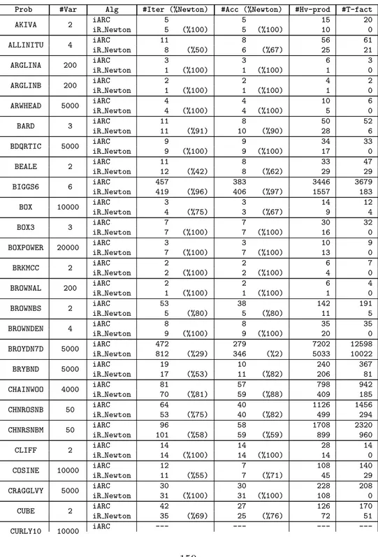
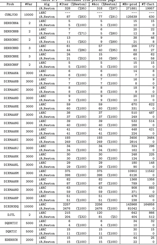
3.4.2 Results on the CUTEst test set . . . 92
4 Complexity Analysis of a Trust Funnel Algorithm for Equality Con-strained Optimization 95 4.1 Preliminaries . . . 96
4.2 Phase 1: Obtaining Approximate Feasibility . . . 97
4.2.1 Step computation . . . 97 4.2.1.1 Normal step . . . 97 4.2.1.2 Tangential step. . . 99 4.2.2 Step acceptance . . . 101 4.2.2.1 F-iteration . . . 102 4.2.2.2 V-iteration . . . 102
4.2.3 Algorithm statement . . . 103
4.3 Convergence and Complexity Analyses for Phase 1 . . . 103
4.3.1 Convergence analysis for phase 1 . . . 104
4.3.2 Complexity analysis for phase 1. . . 119
4.4 Phase 2: Obtaining Optimality . . . 127
4.5 Numerical Experiments . . . 135
5 Conclusion and Future Work 138 5.1 Future Work . . . 139
Bibliography 149 A Subproblem Solver for TRACE 150 B Subproblem Solution Properties and Numerical Results for iR Newton 152 B.1 Subproblem Solution Properties. . . 152
B.2 Subproblem Solution Properties Over Subspaces . . . 154
B.3 Detailed Numerical Results . . . 158
List of Tables
2.1 Percentage of iteration types . . . 65
2.2 Percentage of contraction types . . . 66
3.1 Input parameters foriARC and iR Newton . . . 90
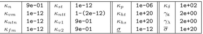
4.1 Input parameters forTFand TF-V-only. . . 136
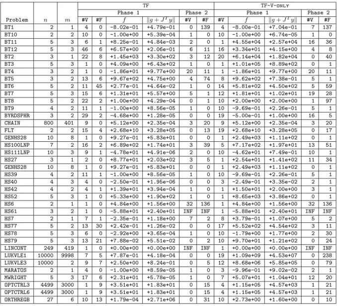
4.2 Numerical results forTFand TF-V-only. . . 137
List of Figures
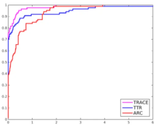
1.1 Inconsistent trust region constraint . . . 20 1.2 Illustration of the trust funnel algorithm . . . 22 1.3 Illustration of Phases 1 and 2 of ShS-ARC . . . 28 2.1 Performance profiles comparing numbers of evaluations, iterations, and
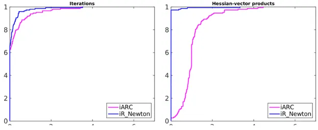
ma-trix factorizations betweentrace,ttr, and arc. . . 66 3.1 Performance profiles foriARC and iR Newton. . . 94
Abstract
For decades, a great deal of nonlinear optimization research has focused on modeling and solving convex problems. This has been due to the fact that convex objects typically represent satisfactory estimates of real-world phenomenon, and since convex objects have very nice mathematical properties that makes analyses of them relatively straightforward. However, this focus has been changing. In various important applications, such as large-scale data fitting and learning problems, researchers are starting to turn away from simple, convex models toward more challenging nonconvex models that better represent real-world behaviors and can offer more useful solutions.
To contribute to this new focus on nonconvex optimization models, we discuss and present new techniques for solving nonconvex optimization problems that possess attrac-tive theoretical and practical properties. First, we propose a trust region algorithm that, in the worst case, is able to drive the norm of the gradient of the objective function below a prescribed threshold of∈(0,∞) after at mostO(−3/2) iterations, function evaluations, and derivative evaluations. This improves upon theO(−2) bound known to hold for some other trust region algorithms and matches the O(−3/2) bound for the recently proposed Adaptive Regularisation framework using Cubics, also known as thearcalgorithm. Our algorithm, entitled trace, follows a trust region framework, but employs modified step acceptance criteria and a novel trust region update mechanism that allow the algorithm to achieve such a worst-case global complexity bound. Importantly, we prove that our algorithm also attains global and fast local convergence guarantees under similar assump-tions as for other trust region algorithms. We also prove a worst-case upper bound on the number of iterations the algorithm requires to obtain an approximate second-order stationary point.
solution in every iteration. This is a reasonable assumption for small- to medium-scale problems, but is intractable for large-scale optimization. To address this issue, the second project of this thesis involves a proposal of a general inexact framework, which contains a wide range of algorithms with optimal complexity bounds, through defining a novel primal-dual subproblem and a set of loose conditions for an inexact solution of it. The proposed framework enjoys the same worst-case iteration complexity bounds for locating approximate first- and second-order stationary points as trace. However, it does not require one to solve subproblems exactly. In addition, the framework allows one to use inexact Newton steps whenever possible, a feature which allows the algorithm to use Hessian matrix-free approaches such as theconjugate gradient method. This improves the practical performance of the algorithm, as our numerical experiments show.
We close by proposing a globally convergent trust funnel algorithm for equality con-strained optimization. The proposed algorithm, under some standard assumptions, is able to find a relative first-order stationary point after at mostO(−3/2) iterations. This matches the complexity bound of the recently proposed Short-Steparc algorithm. Our proposed algorithm uses the step decomposition and feasibility control mechanism of a trust funnel algorithm, but incorporates ideas from our trace framework in order to achieve good complexity bounds.
Chapter 1
Introduction
1.1
Motivation
For decades, the primary aim for many researchers working on solving nonconvex smooth optimization problems has been to design numerical methods that attain global and fast local convergence guarantees. Indeed, a wide variety of such methods have been proposed, many of which can be characterized as being built upon steepest descent, Newton, or quasi-Newton methodologies, generally falling into the categories of line search and trust region methods. For an extensive background on such ideas, one need only refer to numerous textbooks that have been written on nonlinear optimization theory and algorithms; e.g., see [1,3,23,46,57,60]. Worst-case iteration complexity bounds, on the other hand, have typically been overlooked when analyzing nonconvex optimization algorithms. That is, given an objective function f : Rn → R and a sequence of iterates {xk} computed for
solving
min
x∈Rn
f(x), (1.1)
one may ask for an upper bound on the number of iterations required to satisfy
k∇f(xk)k2≤, (1.2)
where∇f :Rn→Rnis the gradient function off and∈(0,∞) is a prescribed constant.
One may also go further and ask for an upper bound on the number of iterations required to satisfy a second-order stationarity condition.
The desire to design fast algorithms is obvious. Analyzing their worst-case iteration complexity, on the other hand, might seem cumbersome and unnecessary to this goal. After all, this is only one factor of the overall performance of an algorithm and it is not always clear that such worst-case analysis accurately represents the typical behavior of an algorithm. Such complexity bounds are typical in the theory of convex optimization algorithms, and are often considered seriously when evaluating such methods. There are numerous examples of scientific efforts in which the process of designing an algorithm with improved worst-case iteration complexity bound enhances the performance of the algorithm in general. One may refer to such advances in the realm of convex optimization, such as the accelerated gradient descent algorithm [53], fast iterative soft thresholding algorithm [2], and interior point methods for linear optimization. Therefore, it seems reasonable for algorithm designers to investigate complexity bounds and develop methods with improved bounds in the field of nonconvex optimization, too.
Traditionally, the most popular methods for solving (1.1) were in classes known as line search and trust region methods. Recently, however, cubic regularization methods have become popular, which are based on the pioneering work by Griewank [45] and Nesterov and Polyak [56]. Their rise in popularity is due to increased interest in algorithms with improved complexity properties, which stems from the impact of so-called optimal algorithms for solving convex optimization problems. The complexity of a traditional trust region method (e.g., see Algorithm 1 in §1.2.2) is O(−2) (see [13] and § 1.2.2), which falls short of theO(−3/2) complexity for cubic regularization methods (e.g., see the arc method by [14,15]). This latter complexity is optimal among a certain broad class of second-order methods when employed to minimize a broad class of objective functions; see [16]. That said, one can obtain even better complexity properties if higher-order derivatives are used; see [8] and [21]. The better complexity properties of regularization methods such asarchave been a major point of motivation for discovering other methods that attain the same worst-case iteration complexity bounds.
In this work, we propose algorithms for nonconvex optimization that attain, under standard assumptions, optimal worst-case iteration complexity bounds. We begin by dis-cussing a (nontraditional) trust region method known astrace(see [28] and Chapter2) with the same optimalO(−3/2) complexity, while at the same time allowing traditional trust region trial steps to be computed and used. We show that these properties can be
realized within the context of a trust region strategy by employing (i) modified step ac-ceptance criteria and (ii) a novel updating mechanism for the trust region radius. Indeed, our acceptance and updating mechanisms represent significant departures from those em-ployed in a traditional approach; e.g., there are situations in which our algorithm may reject a step andexpand the trust region. A key aspect of the trace framework is that a solution to an implicit trust region problem is obtained by varying a regularization pa-rameter instead of a trust region radius. This key idea has been adopted and advanced further by [5]; in particular, they propose an algorithm that has optimal iteration complex-ity by solving quadratic subproblems that have a carefully chosen quadratic regularization parameter.
The algorithm just mentioned is based on the assumption that an exact subproblem solution can be efficiently computed in every iteration. This is a reasonable assumption for small- to medium-scale problems, but is intractable for large-scale optimization. Thus, we extend these ideas for a general inexact regularized Newton framework to improve the practical performance of the algorithm, especially for large-scale problems. In fact, the main contributions of this extension relate to advancing the understanding of optimal complexity algorithms for solving the smooth optimization problem (1.1). Our proposed framework is intentionally very general; it is not a trust region method, a quadratic regu-larization method, or a cubic reguregu-larization method. Rather, we propose a generic set of conditions that each trial step must satisfy that still allow us to establish an optimal first-order complexity result as well as a second-first-order complexity bound similar to the methods above. Our framework contains as special cases other optimal complexity algorithms such asarcand trace (see [30] and Chapter 3).
We also propose a new method for solving equality constrained nonlinear optimization problems. As is well known, such problems are important throughout science and engineer-ing, arising in areas such as network flow optimization [48,58], optimal allocation with re-source constraints [24,49], maximum likelihood estimations with constraints [47], and opti-mization with constraints defined by partial differential equations [4,9,59]. Contemporary methods for solving equality constrained optimization problems are predominantly based on ideas of sequential quadratic optimization (commonly known as SQP) [11,25,26,35– 37,51,57]. The design of such methods remains an active area of research as algorithm developers aim to propose new methods that attain global convergence guarantees under weak assumptions about the problem functions. Recently, however, researchers are being
drawn to the idea of designing algorithms that also offer improved worst-case iteration complexity bounds; e.g., see [17].
For solving equality constrained problems, a cubic regularization method is proposed in [19] with an eye toward achieving good complexity properties. This is a two-phase approach with a first phase that seeks an -feasible point and a second phase that seeks optimality while maintaining -feasibility. The number of iterations that the method re-quires in the first phase isO(−3/2), a bound that is known to be optimal for unconstrained optimization [16]. The authors of [19] then propose a method for the second phase and analyze its complexity properties. Such a two-phase approach is analyzed further—with a careful emphasis on termination conditions for each phase—in [6]. (For related work on cubic regularization methods, see [18, 20].) Notably, the methods in [6, 19] represent a departure from the current state-of-the-art SQP methods that offer the best practi-cal performance; see also [50]. One of the main reasons for this is that contemporary SQP methods seek feasibility and optimality simultaneously. By contrast, the approaches from [6,19] might not offer practical benefits due to the fact that the first phase of each algorithm entirely ignores the objective function, meaning that numerous iterations might need to be performed before the objective function influences the trajectory of the algo-rithm.
Our proposed algorithm can be considered a next step in the design of practical al-gorithms for equality constrained optimization with good worst-case iteration complexity properties. Ours is also a two-phase approach, but is closer to the SQP-type methods rep-resenting the state-of-the-art for solving equality constrained problems. In particular, the first phase of our proposed approach follows a trust funnel methodology that locates an -feasible point in O(−3/2) iterations while also attempting to yield improvements in the objective function. Borrowing ideas from the trust region method known astrace[28] (see Chapter 2), we prove that our method attains the same worst-case iteration complexity bounds as those offered by [6,19].
1.2
Background
Consider an objective functionf :Rn→
R and a starting pointx0∈Rn. For the entirety of this dissertation, we assume thatf is twice continuously differentiable. The main goal
in unconstrained optimization is to find a local solutionx∗ of problem (1.1) such that
f(x∗)≤f(x), for all x∈Rn such thatkx−x∗k2 ≤α and for some α >0.
Many methods have been proposed to solve problem (1.1) with global and fast local convergence guarantees. Global convergence is the ability of converging to a stationary point, which can be a first-order or second-order stationary point, from any remote initial point x0. On the other hand, for local convergence, the rate of convergence to a second-order stationary point is considered when we are in the vicinity of such a point. Indeed, a wide variety of methods with global and fast local convergence properties have been proposed. In this section, we briefly discuss the main methods existing in the literature.
1.2.1 Newton’s method
The standard Newton method is an algorithmic framework in which in every iteration, a quadratic approximation, q, of the objective function f is constructed by using second-order Taylor’s expansion around the current point. The next point is then defined as a minimizer (or approximate minimizer) of the constructed model q. In other words, considering iterationk, we have:
xk+1 =xk+sk, where sk∈arg min s∈Rnqk(s) :=f(xk) +∇f(xk) Ts+1 2s T∇2f(x k)s. (1.3) When∇2f(x
k) is positive definite, the subproblem (1.3) is well-defined and there exists a
closed-form expression for a Newton iteration as the following:
xk+1 =xk−(∇2f(xk))−1∇f(xk).
Newton’s method in its original format as stated in (1.3) is not globally convergent, even for strongly convex problems. Moreover, the solution of subproblem (1.3) is not well-defined when ∇2f(x) is indefinite or negative definite. On the other hand, under some standard assumptions, such as Lipschitz continuity of the Hessian function ∇2f(x) for all xsufficiently close to a nondegenerate second-order stationary pointx∗such that∇2f(x∗)
is positive definite, Newton’s method enjoys a quadratic rate of convergence [31]. This fast local convergence behavior, despite the fact that Newton’s method is not globally convergent, has motivated much research around modifying this method to globalize its convergence properties, such as using Hessian modifications combined with a line search, a trust region methodology, or a regularization approach.
1.2.2 Trust region methods
As mentioned in the last subsection, Newton’s algorithm suffers from the possibility of divergence, but the fast local convergence of this algorithm makes it attractive to explore ways to globalize the method while maintaining its local convergence behavior. Over the years, many variants of Newton’s method with globalization strategies have been developed. For instance, one very popular approach has been to combine line search ideas and Hessian modifications, the latter of which ensures positive definiteness of the Hessian matrices so that the subproblems are well-defined. Another popular approach has been to incorporate trust regions, in which a norm constraint is added to the subproblem to make it well defined, even if the Hessian is not positive definite.
In line search methods, the search direction is chosen or computed first, then the step size is decided, usually based on Armijo-Wolfe conditions [57]. In trust region methods, on the contrary, a region, typically spherical in shape, is defined in which the approximation of the objective function can be “trusted”. Within this “trust region”, a direction is computed that minimizes the model. In a standard trust region method, the trust region is defined by its radius,δ, such that ksk2 ≤δ ; therefore, the trust region subproblem at iteration kis sk∈ min s∈Rn qk(s) =f(xk) +∇f(xk)Ts+ 1 2s T∇2f(x k)s s.t. ksk ≤δk. (1.4)
To ensure the convergence of the algorithm, there are some rules used to update the trust region radius. Any reasonable updating procedure has to consider the quality of the step computed in each iteration; therefore, defining a proper measure of solution quality is critical for the convergence of this algorithm. One popular quality measure in the literature constructs the ratio of “actual reduction” over “predicted reduction” of the objective value, calledρkat iterationk, and compares the resulting ratio with a pre-specified constantη. If
ρk≥η, then the trial step computed by solving (1.4) will be accepted; otherwise, the trial
step will be rejected. In the latter case, an update inδ is necessary to generate a different solution in the next step. As the Taylor approximation is more accurate within a smaller region, a proper update is to decrease the trust region radius for the next iteration. While not necessary,δ will be increased for the caseρk ≥η, with the hope of faster convergence.
Algorithm 1 is a common representation of a standard trust region method [23].
Algorithm 1 Trust Region Method
Require: an acceptance constantη ∈R++ with 0< η <1 Require: update constants{γc,γe} ⊂R++ with 0< γc<1< γe
1: choosex0∈Rn,δ0∈R++
2: fork= 0, 1, 2,. . . do
3: computesk by solving (1.4)
4: computeρk as the following:
ρk :=
f(xk)−f(xk+sk)
f(xk)−qk(sk)
(1.5)
5: if ρk≥η then [accept step and expand trust region]
6: setxk+1←xk+sk
7: setδk+1←max{δk,γekskk2}}
8: else (ρk < η) [reject step and contract trust region]
9: setxk+1←xk
10: setδk+1←γckskk2
Under some standard assumptions, such as Lipschitz continuity of the gradient func-tion ∇f, Algorithm 1 enjoys global convergence. In addition, under the assumption of Lipschitz continuity of ∇2f for all x sufficiently close to a nondegenerate second-order stationary point x∗ such that ∇2f(x∗) is positive definite, this algorithm has quadratic
local convergence, similar to Newton’s method [57].
1.2.2.1 Worst-case first-order complexity of trust region methods
Despite the good performance that people have seen for trust region methods, in terms of their complexity, one can show that they might require O(−2) iterations to find an -stationary point. In fact, an example, constructed by Cartis, Gould, and Toint [13], shows that for anyτ >0, Newton’s method needs at leastO(−2+τ) iterations to achieve the stationarity measure tolerance (1.2). The same example can be used to show that the traditional trust region Algorithm1 follows the same steps similar to those generated by
Newton’s method [16].
Consider the following two-dimensional example in which the sequence{xk}is the one
that would be generated by Newton’s method:
x0 = (0, 0)T, xk+1=xk+sk, sk = 1 k+1 12+¯τ 1 , (1.6a) f(x0) = 1 2[ζ(1 + 2¯τ) +ζ(2)], f(xk+1) =f(xk)− 1 2 " 1 k+ 1 1+2¯τ + 1 k+ 1 2# , (1.6b) ∇f(xk) =− 1 k+1 1 2+¯τ 1 k+1 12 , (1.6c) and ∇2f(xk) = 1 0 0 k+11 2 , (1.6d) where ¯τ = τ /(4−2τ) > 0 and ζ(t) := P∞
k=1k−t is the Riemann ζ function [13]. With the sequence of gradients as in (1.6c), the number of iterations needed to satisfy the stationarity measure tolerance (1.2) is at leastO(−2+τ). For the defined sk,∇f(xk), and ∇2f(x
k), we have
∇2f(xk)sk=−∇f(xk),
with positive definite∇2f(x
k); therefore, sk globally minimizes qk(s). Furthermore,
f(xk+sk) =qk(sk),
which guaranteesρk= 1; therefore, according to Step5, the trial stepskwill be accepted.
The definition of sk in (1.6a) guarantees that ksk+1k2 < kskk2 for all k ≥ 0. On the other hand, from ρk = 1, Step 5, and Step (7), one can deduce that δk+1 ≥ δk for all
k≥0. If δ0 ≥ ks0k2 = √
2, then the sequence of{xk}defined in (1.6a) can be reached by
applying the traditional trust region Algorithm1to minimizing a function satisfying (1.6); therefore, Algorithm 1 requires at least O(−2+τ) iterations to achieve the stationarity
measure tolerance (1.2).
Hermite interpolation on the interval [0,xk+1−xk]. To do so, consider
f(x) =f1([x]1) +f2([x]2), (1.7)
where [x]i is the i-th component of x for i∈ {1, 2}. Using Hermite interpolation, for all
k≥0 we have
f1([x]1) =pk([ˆx−xk]1) +f1([xk+1]2) for [ˆx]1 ∈[[xk]1, [xk+1]1] , (1.8)
wherepk is the polynomial
pk(s) =c0,k+c1,ks+c2,ks2+c3,ks3+c4,ks4+c5,ks5, (1.9)
with coefficients defined to satisfy the interpolation conditions
pk(0) = 1 2 1 k+ 1 1+2¯τ , pk([sk]1) = 0; ∇pk(0) =− 1 k+ 1 12+¯τ , ∇pk([sk]1) =− 1 k+ 2 12+¯τ ; ∇2pk(0) = 1, ∇2pk([sk]1) = 1. (1.10)
In addition, for the univariate functionf2 we have for allk≥0
f2([x]2) =wk([ˆx−xk]2) +f1([xk+1]2) for [ˆx]2 ∈[[xk]1, [xk+1]2] , (1.11)
wherewk is the polynomial
wk(s) =d0,k+d1,ks+d2,ks2+d3,ks3+d4,ks4+d5,ks5, (1.12)
with coefficients defined to satisfy the interpolation conditions
wk(0) = 1 2 1 k+ 1 2 , wk(1) = 0; ∇wk(0) =− 1 k+ 1 2 , ∇wk(1) =− 1 k+ 2 2 ; ∇2wk(0) = 1 k+ 1 2 , ∇2wk(1) = 1 k+ 2 2 . (1.13)
Therefore, according to [13] c0,k= 1 2 1 k+ 1 1+2¯τ , c1,k=− 1 k+ 1 1 2+¯τ , c2,k= 1 2 c3,k= 4 (k+ 1)2 k+ 2 !12+¯τ c4,k=−7 (k+ 1)3 k+ 2 !12+¯τ c5,k= 3 (k+ 1)4 k+ 2 !12+¯τ . (1.14) Furthermore, according to [13] d0,k= 1 2 1 k+ 1 2 , d1,k=− 1 k+ 1 2 , d2,k = 1 2 1 k+ 1 2 d3,k= 9 2 1 k+ 2 2 −1 2 1 k+ 1 2 d4,k=−8 1 k+ 2 2 + 1 k+ 1 2 d5,k= 7 2 1 k+ 2 2 − 1 k+ 1 2 . (1.15)
The proofs of Lipschitz continuity of∇f(x) and∇2f(x) and boundedness off are pre-sented in [13]; therefore, the function f constructed this way satisfies all the assumptions needed for convergence of Algorithm 1. This example shows that trust region methods can be inefficient, in the sense that they might takeO(−2) iterations to achieve the sta-tionarity tolerance (1.2). In the next subsection, we turn to an alternative framework that achieves improved worst-case iteration complexity over trust region methods.
1.2.3 Cubic regularization methods
As mentioned, worst-case iteration complexity bounds have typically been overlooked when analyzing nonconvex optimization algorithms. This situation in the field of non-convex optimization has started to change with recent studies on cubic regularization methods. Originally proposed in a technical report by Griewank [45], the foundation for
worst-case iteration complexity bounds for second-order methods using cubic regulariza-tion was first established in the seminal work by Nesterov and Polyak [56]. (See also [61] for another early article on such methods.) Nesterov and Polyak [56] proposed and ana-lyzed an abstract algorithm called Cubic regularization of Newton Method (or CNM as referred to in [55]). In this algorithm, to overcome issues related to ill-defined subproblems when the Hessian is indefinite, a cubic term is added to the quadratic model qk(s). The
resulting subproblem is an unconstrained (potentially) nonconvex cubic problem
sk∈arg min s∈Rn ck(s) :=f(xk) +∇f(xk)Ts+ 1 2s T∇2f(x k)s+ σk 6 ksk 3 2,
where σk is the algorithm parameter whose value is set in every iteration to satisfy a
so-called sufficient decrease property defined as
f(xk+sk)≤c(sk). (1.16)
The inequality (1.16) is satisfied for everyσk≥L, whereLis the Lipschitz constant of the
Hessian function ∇2f(x); therefore, a procedure of increasing σ
k by multiplying with a
constant will eventually terminate after satisfying (1.16). Algorithm2 shows the original CNM algorithm from [56].
Algorithm 2 Cubic regularization of Newton Method (CNM) Require: a constantL0∈R++ withL0≤L
1: choosex0∈Rn
2: fork= 0, 1, 2,. . . do
3: findσk∈[L0, 2L] such that (1.16) is satisfied
4: set xk+1←xk+sk
The global convergence of Algorithm 2 to a second-order stationary point is proved under the assumption of Lipschitz continuity of∇fand∇2f. While the former assumption is pretty standard in the literature for convergence, the latter one seems strong because it assumes global Lipschitz continuity of the Hessian, not just near a minimizer. But, one should notice that they have proved the convergence to a local solution x∗ satisfying the second-order sufficient condition, that is∇f(x∗) = 0 and∇2f(x∗) is positive semidefinite.
In addition, there exist several lemmas and theorems in their paper from which the worst-case iteration complexity bound ofO(−3/2) to a first-order stationary point and O(−3)
to a second-order stationary point can be inferred for successful (those satisfying (1.16)) iterations.
Despite the salient properties of Algorithm 2, it is far away from being a practical algorithm. First of all, the Lipschitz continuity of the Hessian function might be a strong assumption for those who only need the convergence to a stationary point with zero gradient. Second, the assumption of knowing the Lipschitz constant L beforehand to use in the algorithm is extremely restrictive. Last but not least, finding σk ∈ [L0, 2L] satisfying (1.16) as the way stated in Algorithm 2 might not be efficient in terms of complexity bounds.
More recently, the Adaptive Regularisation framework using Cubics, also known as thearcalgorithm [14,15], was developed with an eye towards practical implementations. In this work as in [56], Cartis, Gould, and Toint propose an algorithm in which the trial steps are computed by minimizing a local cubic model of the objective function at each iterate. The expense of this computation is similar to that of solving a subproblem arising in a typical trust region method, and their overall algorithm—which has essentially the same flavor as a trust region method—is able to attain global and fast local convergence guarantees. However, the distinguishing feature of arc and other cubic regularization algorithms is that, under reasonable assumptions, they ensure that the stationarity mea-sure tolerance (1.2) is guaranteed to hold after at mostO(−3/2) iterations. Furthermore, the analysis in [16] shows that the complexity bound for arc is optimal with respect to a particular class of second-order methods for minimizing a particular class of sufficiently smooth objective functions in the optimization problem (1.1).
Inarc, the subproblems are similar to CNM, where a cubic regularization of a second-order Taylor series will be solved, namely
sk∈arg min s∈Rn Ck(s) :=f(xk) +∇f(xk)Ts+ 1 2s TB ks+ σk 3 ksk 3 2, (1.17)
whereBk is an estimation of ∇2f(xk) and σk is the algorithm parameter whose value is
updated dynamically by the algorithm. To measure the quality of the trial stepsk, a ratio
of actual reduction over predicted reduction is computed as the following:
ρCk := f(xk)−f(xk+sk) f(xk)−Ck(sk)
Then, based on this ratio the acceptance or rejection of the trial step is decided, moreover, σk+1 is set properly. Algorithm3 shows thearc algorithm.
Algorithm 3 Adaptive Regularization using Cubics (ARC)
Require: two acceptance constants{η1,η2} ⊂R++ with 0< η1< η2<1
Require: update constants{γ1,γ2} ⊂R++ with 1< γ1< γ2
1: choosex0∈Rn,δ0∈R++ 2: fork= 0, 1, 2,. . . do 3: computesk by solving (1.17) 4: computeρCk using (1.18) 5: if ρCk ≥η1 then 6: setxk+1←xk+sk 7: if ρCk ≥η2then 8: setσk+1∈[0,σk] 9: else(η1< ρCk < η2) 10: setσk+1∈[σk,γ1σk] 11: else (ρC k < η) 12: setxk+1←xk 13: setσk+1∈[γ1σk,γ2σk]
Because of the importance of the arc algorithm in the development and analysis of our proposed algorithms described in later chapters, a more official statement of the convergence properties and the complexity bounds of this algorithm is presented in the following theorem.
Theorem 1. Suppose thatf :Rn→Ris continuously differentiable and the sequence{fk}
is bounded from below. If the gradient function is Lipschitz continuous and Bk is bounded
in norm for all k, then {∇f(xk)} →0. Furthermore, if f is twice continuously
differen-tiable, Bk is a relatively close approximation of ∇2f(xk) such thatkBk− ∇2f(xk)k2 →0
wheneverk∇f(xk)k2→0andk→ ∞, and there exists a subsequence of iterates converging
tox∗with positive definite∇2f(x∗), then the whole sequence{x
k}converges tox∗. In
addi-tion, if ∇2f(x)is locally Lipschitz continuous close tox∗,k(B
k− ∇2f(xk))skk2 ≤Ckskk22,
for allk, and some constantC >0, and σk ≥σmin for allkand some constantσmin>0,
then xk→x∗ and∇f(xk)→0 Q-quadratically. Moreover, if ∇2f(x) is globally Lipschitz
continuous on the path of computed iterates, then the whole sequence{xk}converges tox∗
with ∇f(x∗) = 0 and positive semidefinite ∇2f(x∗) from any remote initial pointx
0.
With the same assumptions, for any ¯ > 0, the stationarity measure tolerance (1.2) is guaranteed to hold after at most O(−3/2) iterations, where ∈ (0, ¯]. In addition,
the number of iterations required to find a point xk such that the smallest eigenvalue of ∇2f(x
k) is greater than or equal to −is at most O(−3).
Although in Step3of Algorithm3the global solution of (1.17) is considered assk, for
Theorem1to be valid, such a solution is not required, butsk needs to be a global solution
for (1.17) on a subspace containing the gradient∇f(xk) with
k∇Ck(sk)k2 ≤θk∇f(xk)k, (1.19)
for some constantθ >0. This milder requirement makesarcmore practical especially for large-scale problems where solving the nonconvex problem (1.17) might be prohibitively expensive. Under this more relaxed assumption,sk must satisfy the following condition:
∇f(xk)Tsk+sTkBksk+σkkskk3 = 0, (1.20)
(which is equivalent to∇Ck(sk)Tsk= 0) and
sTkBksk+σkkskk3 ≥0. (1.21)
The importance of the improvement in the complexity bound gets more noticeable when it is compared to the trust region method. As one may notice that Algorithms 1 and 3 are very similar in terms of the framework. In fact, the similarity of these methods are not restricted only to the framework; the subproblem solutions can be the same if one chooses the appropriate parameters. For example, the solution sk of (1.17) is also
an optimal solution for (1.4) if δk is set to kskk2. Furthermore, an optimal solution sk
for (1.4) is also an optimal solution for (1.17) with σk =λk/kskk2, where λk is the dual
variable associated with the trust region constraint.
Despite the improved worst-case iteration complexity bounds of arc, there is not a noticeable performance improvement versus trust region method, yet in many cases, the trust region algorithm, even in its standard version, beats the arc algorithm in terms of solution time and even iterations needed to satisfy a measure of convergence as (1.2). One of the main motivations of this dissertation is to answer the question if there exists a trust region method with improved iteration complexity bounds as those of arc. In the next chapter, we answer this question.
Our motivation of proposing a new trust region algorithm is to introduce an algo-rithm which can perform well in practice while theoretically achieves improved complexity bounds. To this end, an inexact regularized Newton framework is proposed in Chapter3, which allows inexact Newton steps whenever possible while achieves the improved worst-case iteration complexity bounds, similar to those of arcand trace.
1.2.4 Methods for equality constrained problems
In real world problems, the decision variablexin problem (1.1) might need to be restricted, e.g., due to resource limitations, state and federal regularizations, technology bounds, and engineering designs. Therefore, many optimization problems are “constrained” problems of the form
min
x∈Xf(x), (1.22)
where X is the set of all possible decisions defined by constraints. The set X in (1.22) might possess different properties; e.g., it might be convex or not convex, closed or open, connected or disconnected, etc. In this work, instead of the general form (1.22), we assume that X can be defined by a multivariate continuous function c : Rn → Rm such
thatX ={x∈Rn|c(x) = 0}; therefore, we assume thatX is closed. For some algorithms,
there might be other assumptions oncsuch as differentiability, smoothness, and so-called constraints qualifications. The constrained problem, then, will be defined as the following:
min
x∈Rn
f(x)
s.t. c(x) = 0.
(1.23)
The widespread application of (1.23) has motivated an enormous deal of research to develop “reliable” algorithms to solve it. The term “reliable” itself needs clarification; for us, a very loose definition of a reliable algorithm can be expressed as an algorithm with the ability to find a pointx∗ or generate a sequence of points {xk}converging to x∗ that
satisfies the Karush-Kuhn-Tucker (KKT) optimality conditions of (1.23) or, in the case of an infeasible instance of (1.23), a sequence converging to a stationary point c. Once again, the main body of research for many years was focused on designing algorithms with global convergence properties and, similar to the unconstrained case, the analysis of the worst-case iteration complexity bounds is a recent trend on this area; e.g., see the recent
work in [18–20].
Before going any further, let us define the KKT optimality conditions. The Lagrangian function of (1.23) is defined as L(x,y) := f(x) +c(x)Ty. Let f and c be continuously differentiable. The pair (x,y) is a KKT point if:
∇f(x) +∇c(x)Ty= 0 c(x) = 0.
(1.24)
KKT conditions are necessary for any optimal (local or global) solution if some sort of constraint qualification, such as the Linear Independence constraint qualification (LICQ) [57], holds. Similar to the unconstrained case, there are also second-order optimality conditions givenf and care twice continuously differentiable.
1.2.4.1 Sequential quadratic programming
Similar to unconstrained optimization algorithms, one may consider to iteratively solve a model of problem (1.23) and take the step found by solving the model. Sequen-tial Quadratic Programming/Optimization (SQP) is a well-known iterative framework in which a second-order model of the objective function and a linearization of the con-straint functions are considered as a model of the original problem (1.23), leading to a subproblem of the form
min s∈Rn f(x) +∇f(x)Ts+1 2s TBs s.t. c(x) +∇c(x)s= 0, (1.25)
where B is positive definite. The optimality conditions (KKT conditions) for problem (1.25) are
∇f(x) +Bs+∇xc(x)Tη= 0
c(x) +∇xc(x)s= 0,
(1.26)
where η is an m×1 vector of dual variables for problem (1.25). We can rewrite these linear equations in matrix form as
B ∇c(x)T ∇c(x) 0 s η =− ∇f(x) c(x) . (1.27)
If one applies Newton’s method to solve (1.24), one will have the following linear system of equations: ∇2 xxL(x,y) ∇c(x)T ∇c(x) 0 ∆x ∆y =− ∇f(x) +∇c(x)Ty c(x) . (1.28)
A closer look to two equations (1.28) and (1.27) shows that these two equations are exactly the same if we setB =∇2
xxL(x,y) and η =y+ ∆y. This observation shows that solving
the problem (1.23) by using SQP is exactly the same as solving the KKT conditions (1.24) by using Newton’s method; therefore, the SQP algorithm in its original form is not globally convergent. Hence, combining other globalization frameworks such as line search or trust region strategies is required. In addition, to be able to analyze the SQP method, assuming that the KKT conditions are necessary is a standard assumption. This can be done, e.g., by making the following assumption.
Assumption 1. The matrix ∇c(x∗) has full row rank for any x∗ ∈arg minx∈Xf(x).
Assumption 1 means that the LICQ is satisfied at x∗; so the KKT conditions are necessary for any minimizer of (1.23).
Another typical assumption is the following.
Assumption 2. It holds that dT∇2
xxL(x,y)d≥0 for all dsuch that ∇c(x)Td= 0.
Assumption2is useful to guarantee local convergence when we are in a vicinity of x∗, because positive definiteness of∇2
xxL(x,y) is essential for fast local convergence of SQP.
1.2.4.2 SQP with a trust region constraint
In the case of SQP, similar to the unconstrained case for Newton’s method, to make the algorithm globally convergent, using a line search, trust region framework, or other globalization mechanism is required. Here, we discuss the use of trust regions to globalize the method. In trust region methods, we try to find a solution for the model within a “trusted” area which the original function is believed to behave almost the same as the estimated function. In our present case, this leads to a subproblem of the form
min s∈Rn f(x) +∇f(x) Ts+1 2s TBs s.t. c(x) +∇c(x)s= 0 ksk ≤δ, (1.29)
whereδ is the trust region radius.
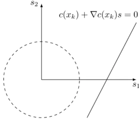
A challenge in constrained optimization is the possibility of achieving an inconsistent subproblem by adding a trust region constraint. This will make the algorithm not well defined unless modifications are made. Figure 1.1 shows such a subproblem in a two-dimensional space.
s1
s2
c(xk) +∇c(xk)s= 0
Figure 1.1: Inconsistent trust region constraint
Several tricks have been proposed to handle this problem [57], but among all of them, we will discuss the step decomposition strategy. In this procedure, the step sk
is decomposed into two components: nk and tk (where nk should not be confused with
the number of variables n). The first one, nk is chosen to find the minimum value of kc(xk) +∇c(xk)nkk22 within the trust region (or as it is the most common, into a region smaller than the original trust region). Then, tk is chosen in the null space of ∇c(xk),
N(∇c(xk)) :={x∈Rn | ∇c(xk)x= 0}, to solve a possibly modified version of (1.29): min s∈Rn f(xk) +∇f(xk)Ts+ 1 2s TB ks s.t. c(xk) +∇c(xk)s=c(xk) +∇c(xk)nk ksk ≤δ, (1.30)
wheresk=nk+tk. Although not always necessary,nk is commonly assumed to be in the
range space of∇c(xk)T, R(∇c(xk)T) :={∇c(xk)Tx | x∈ Rm}, which is why it is called the “normal” step. In addition,tk is called the “tangential” step as it is in the null space
of∇c(xk). (Notice that for any matrix A, the range space of AT and the null space ofA
are orthogonal spaces.)
Another issue that we have to consider in designing a trust region SQP algorithm is the definition of a good measure for progress such as a merit function. In unconstrained problems, the natural merit function is simply f itself, but for constrained problems, a merit function has to consider feasibility as well as the objective function value. For a complete review of these issues and the possible solutions, one may refer to numerous references such as [57].
The next two subsections are dedicated to two globally convergent algorithms for solving (1.23) with two completely different approaches to solve these above-mentioned issues and also with two different design objectives. The trust funnel algorithm is a method based on a step decomposition strategy in which the main goal is to generate a globally convergent algorithm. The Short Step arc (ShS-ARC) algorithm, on the other hand, is designed to achieve not only global convergence but also to guarantee good worst-case iteration complexity bounds for solving constrained problems. In this algorithm, subproblems are unconstrained, so inconsistency of the subproblems is not an issue.
1.2.4.3 Trust funnel algorithm
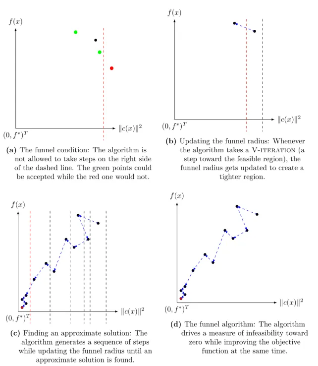
A recent algorithmic framework with global convergence guarantees [27, 38] based on a step decomposition strategy will be discussed here. We present this algorithm in details as it will be used in our proposed new algorithm with good worst-case iteration complexity bounds in Chapter4. The trust funnel algorithm attempts to drive a measure of infeasi-bility to zero at the same time that it tries to improve the objective value. In particular,
progress towards reducing the constraint violation measures is guided by a tolerance that is reduced dynamically by the algorithm. (See Figure1.2.)
(0,f∗)T
kc(x)k2
f(x)
(a)The funnel condition: The algorithm is not allowed to take steps on the right side of the dashed line. The green points could be accepted while the red one would not.
(0,f∗)T
kc(x)k2
f(x)
(b)Updating the funnel radius: Whenever the algorithm takes aV-iteration(a step toward the feasible region), the funnel radius gets updated to create a
tighter region.
(0,f∗)T kc(x)k
2
f(x)
(c) Finding an approximate solution: The algorithm generates a sequence of steps while updating the funnel radius until an
approximate solution is found.
(0,f∗)T
kc(x)k2
f(x)
(d) The funnel algorithm: The algorithm drives a measure of infeasibility toward
zero while improving the objective function at the same time.
For equality constrained problems, a reasonable measure of infeasibility can be defined as the sum of squares of the constraint values, or equivalently, a function v :Rn → R is defined which measures the infeasibility of a pointx as the following:
v(x) := 1 2kc(x)k
2
2. (1.31)
During the running of the algorithm, the hope is that the value of v converges to zero while the solution approaches to a stationary point of the Lagrangian function
L(x,y) :=f(x) +yTc(x); (1.32)
otherwise the algorithm fails in finding a first-order stationary point of the problem. In addition, we definevmax as a dynamic parameter, whose value is set in each iteration such
that vmax
k+1 ≤vkmax. The trial step sk can be accepted only if v(xk+sk) ≤ vkmax, which is
called the funnel condition.
In a typical trust funnel algorithm, three vectors are computed in each iterationk: the normal step nk, the tangential step tk, and the multiplier estimate yk. The vector nk is
the step taken to minimize the Gauss-Newton approximation of the functionv, subject to a trust region constraint, defined as the following:
nk∈arg min n∈Rn m v k(n) := 1 2kc(xk) +∇c(xk)nk 2 2 s.t. knk2 ≤δkv, (1.33)
where δkv is the trust region radius for normal step at iteration k. After finding nk, an
estimate of the Lagrangian multiplieryk is computed:
yk∈arg min y∈Rm 1 2k∇f(xk) +∇ 2f(x k)nk+∇c(xk)Tyk22. (1.34)
Problem (1.34) tries to find multiplieryksuch that the difference of−∇f(xk)−∇2f(xk)nk
(an approximation of the negative gradient of the objective atxk+nk) and∇c(xk)Tykgets
the minimum possible value. This, in turn, means thatykis found such that∇c(xk)Tyk is
the projection of−∇f(xk)− ∇2f(xk)nk ontoR(∇c(xk)T). Hence,∇f(xk) +∇2f(xk)nk+ ∇c(xk)Tyk is the projection of −∇f(xk)− ∇2f(xk)nk onto N(∇c(xk)). To justify the
point xk, KKT conditions are satisfied for the pair (xk,yk), where yk is computed from
(1.34).
After computingnkand yk, the tangential steptk is determined to solve the following
problem: tk ∈arg min t∈Rn mfk(nk+t) :=f(xk) +∇c(xk)T(nk+t) + 1 2(nk+t) T∇2f(x k)(nk+t) s.t. ∇c(x)t= 0 knk+tk2 ≤δks, (1.35) where δsk is the radius of the region within which both constraint model and objective function model can be trusted. To this end, one may define δks := min{κvδkv,δkf}, where
κv ∈R++withκv >1 andδkf is the trust region radius for objective model. Another reason
for using (1.34) to estimateyk relates to the fact that ∇f(xk) +∇2f(xk)nk+∇c(xk)Tyk
is in N(∇c(xk)); thus, this vector can be used as an initial search direction for (1.35).
In fact, for convergence purposes there is no need to solve (1.35) exactly, while finding a solution which is at least as good as the optimal solution in the direction of ∇f(xk) + ∇2f(x
k)nk+∇c(xk)Tyk (sometimes referred to as the Cauchy direction) suffices.
After finding the normal step, new multiplier, and tangential step, the algorithm de-cides to perform a so-calledF-iteration orV-iterationbased on the properties of the trial stepsk :=nk+tk. In anF-iteration, the main focus is on decreasing the objective function value while the main focus in an V-iteration is on decreasing the infeasibility measure,v. After finding the trial stepsk, a set of simple conditions is checked to find the
eligibility of anF-iteration. In a typical trust funnel algorithm, these conditions are
tk6= 0 (1.36a) v(xk+nk+tk)≤vmaxk (1.36b) mfk(0)−mfk(nk+tk)≥κ mfk(nk)−mfk(nk+tk) , whereκ∈(0, 1). (1.36c)
If the conditions for performing anF-iterationare not satisfied, then aV-iteration is performed. In both anF-iterationand aV-iteration, the acceptance of the trial step and updating of the trust region radius follow by trust region rules. In a V-iteration, the quality of the trial step based on the infeasibility measure decrease is explored, then
accordingly, the funnel radius vmax
k+1 is set. Algorithm4 shows a version of a trust funnel algorithm [27].
Algorithm 4 Trust Funnel Algorithm
Require: an acceptance constantη∈R++for accepting steps inF-iterationandV-iteration,
with 0< η < 1, some constants: 0 < κ < 1, κv >0, κf v >0, 0 < κcs ≤1, 0 < κns ≤1,
κts1>0, and 0< κts2<1.
Require: a constantθ∈R++ with 0< θ <1 which identifies the fraction of trust region radius
in computing normal step.
Require: bound constants{σ,σ} ⊂R++ with 0≤σ≤σ;
1: procedureTrust Funnel Algorithm
2: choose x0∈Rn,y−1∈Rm+,v0max≥max{1,v(x0)},δ
f
0 ∈R++,δv0∈R++
3: fork= 0, 1, 2,. . . do
4: calculatevk
5: if ck6= 0 then
6: compute normal step,nk, using (1.33);
7: else
8: setnk ←0;
9: compute the Lagrangian multiplier,yk, using (1.34);
10: calculategk+Hknk+JkTyk;
11: if ck= 0 and gk+Hknk+JkTyk = 0then
12: terminate.
13: compute tangential step,tk, using (1.35);
14: setsk ←nk+tk;
15: if (1.36) is satisfiedthen [F-iteration]
16: setvmax k+1←v max k 17: computeρfk := f(xk)−f(xk+sk) mfk(0)−mfk(sk) ; 18: if ρfk≥η then 19: setxk+1←xk+sk,δkv+1≥δvk,δ f k+1≥δ f k 20: else 21: setxk+1←xk,δvk+1←δkv,δ f k+1∈(0,δ f k) 22: else [V-iteration] 23: setδkf+1←δkf 24: computeρvk := v(xk)−v(xk+sk) mv k(0)−m v k(sk) ; 25: if ρv k≥η then 26: setxk+1←xk+sk,δkv+1≥δ v k,v max k+1∈(0,v max k ) 27: else 28: setxk+1←xk,δvk+1∈(0,δ v k),v max k+1←v max k
Algorithm 4 is globally convergent [27, 38]. However, to the best of our knowledge, its complexity properties have not been studied in detail. In Chapter 4, we propose a modification of this framework with good worst-case complexity bounds. Our algorithm
borrows many ideas from the method proposed in Chapter2.
1.2.4.4 The Short-Step ARC (ShS-ARC) algorithm
The success of arc in approximately solving unconstrained problems within O(−3/2) iterations drew researchers’ attention to designing algorithms with improved iteration complexity bounds for constrained optimization. Cartis, Gould, and Toint explored the complexity of constrained optimization [18,19]. Particularly, in [19], they introduce a two-phase method for (1.23), where in both phasesarcwas used. They analyze the worst-case iteration complexity bound of the proposed algorithm to locate a relative KKT point and prove that it can even be as good asO(−3/2), under some assumptions.
In the Short-Step arc (ShS-ARC) algorithm (see Algorithm 5), the first phase is used to find a (relatively) feasible point by usingarc to minimize 12kc(x)k2
2. The second phase, on the other hand, is trying to decrease the objective function within the relative feasible region through a so-called “target following” strategy. During the second phase, a target valuetfor the objective function is introduced. Then, arcis used to reduce the 1 2kr(x,t)k22, where r(x,t) := c(x) f(x)−t . (1.37)
The target valuetis carefully chosen and iteratively decreased until the termination con-dition is satisfied. The termination concon-ditions involve a function called “scaled gradient” as a measure of optimality such that
gr(x,t) := ∇c(x)Tc(x)+(f(x)−t)∇f(x) kr(x,t)k2 whenever r(x,t)6= 0, 0 otherwise. (1.38)
Phase 1 terminates either with an approximately feasible pointx0such thatkc(x0)k2 ≤ p or an approximate infeasible first-order stationary point of kc(x)k2. The number of Phase 1 iterations to generate a point with kc(x1)k2 ≤ p or norm of its gradient,
k∇c(x1)Tc(x1)k2
kc(x1)k2 ≤ d is at most O(
−3/2) with = min{
p,d}. In Phase 2, on the other
hand, the algorithm starts from an approximately feasible pointx1 generated by Phase 1, keeps the relative feasibility such that for all iterationk ≥0, kc(xk)k2 ≤p while trying
Algorithm 5 The Short-Step arc(ShS-ARC) algorithm Require: a starting pointx0,
Require: initial regularization parameters σ0 and σ1 and a minimal one σmin such that
min{σ0,σ1} ≥σmin>0,
Require: algorithmic parametersγ2≥γ1>1 and 1> η2≥η1>0,
Require: the tolerancesp∈(0, 1) andd∈(0, 1).
1: procedurePhase 1
2: starting fromx0, applyarcto minimize 12kc(x)k22 until a pointx1 is found such that
kc(x1)k2≤p or
k∇c(x1)Tc(x1)k2
kc(x1)k2
≤d. (1.39)
3: if kc(x1)k2> p then
4: terminate. (locally infeasible)
5: procedurePhase 2 6: set t1←f(x1)− q 2 p− kc(x1)k22andk←1 7: fork= 1, 2,. . . do
8: starting fromxk, apply one iteration of arcto approximately minimize 1 2 c(xk)T,f(xk)−tk2 9: if ρC k ≥η1then 10: if kgr(xk+1,tk)k2≤d andr(xk+1,tk)6= 0then 11: terminate. 12: else 13: set tk+1=f(xk+1)− q kr(xk,tk)k22− kr(xk+1,tk)k22+ (f(xk+1−tk)2. 14: else 15: settk+1 ←tk
{tk}, such that |f(xk)−tk| ≤p. All these are guaranteed by the definition of t1 in Step
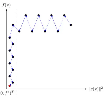
6 and the updating oftk in Steps13 and 15. Illustration of Phases 1 and 2 of ShS-ARC
can be seen in Figure1.3.
When Phase 2 terminates, we are either at an approximate stationary point ofkc(x)k2 withf(x) =t, or at a relative KKT point with f(x)6=t([19], Lemma 4.2) such that
k∇c(x)Ty(x,t) +∇f(x)k2
(0,f∗)T kc(x)k
2
f(x)
Figure 1.3: Illustration of Phases 1 and 2 of ShS-ARC
where
y(x,t) := c(x)
|f(x)−t|.
In [19], the authors have justified the condition (1.40) by a perturbation argument: Con-siderx=x∗+δxandy=y∗+δy where (x∗,y∗) is the primal-dual pair satisfying KKT
con-ditions. Then, a first-order Taylor’s expansion of∇c(x∗)Ty∗+∇f(x∗) to estimate its value at the perturbed point (x,y) will give us the estimation ∇2f(x∗) +Pm
i=1yi∗∇2ci(x∗)δx+ ∇c(x∗)Tδy. The presence of dual variabley∗ in this estimation justifies that the magnitude
of the dual variable should not be ignored in relative KKT point condition as in (1.40). In the next theorem, the iteration complexity bound for Algorithm5and the required assumptions are represented from [19].
Theorem 2. Assume that:
• The function cis twice continuously differentiable onRn andf is twice continuously differentiable in a sufficiently large open set containing C1 := {x ∈ Rn | kc(x)k2 ≤ κc}, where κc> p.
globally Lipschitz continuous on the path of all Phase 1 and Phase 2 iterates and trial points.
• f(x), ∇f(x), and ∇2f(x) are globally Lipschitz continuous on the path of all Phase
2 iterates and trial points.
• The objective function f(x) is bounded above and below in C1.
In addition, considerd≤1p/3. Furthermore, assume that the Hessian approximates used
in arc subproblems to minimize 12kc(x)k2
2 in Phase 1 and 12kr(x,tk)k 2
2 in Phase 2 are
relatively accurate. Then, Algorithm5 generates an iterate xk satisfying either a relative
KKT condition for (1.23) with
kc(xk)k2≤p and
k∇c(xk)Tyk+∇f(xk)k2 k(yk, 1)k2
≤d
for some yk ∈Rm, or an approximate first-order stationary point forkc(x)k2 with
k∇c(xk)Tc(xk)k2 kc(xk)k2
≤d
in at most O(−d3/2p−1/2) evaluations of c and f and their derivatives. Therefore, if one
chooses := d = 2/3
p