F
Robust Face Recognition With Kernelized
Locality-Sensitive Group Sparsity Representation
Shoubiao Tan, Xi Sun, Wentao Chan, Lei Qu, and Ling Shao
Abstract— In this paper, a novel joint sparse representation method is proposed for robust face recognition. We embed both group sparsity and kernelized locality-sensitive constraints into the framework of sparse representation. The group sparsity constraint is designed to utilize the grouped structure information in the training data. The local similarity between test and training data is measured in the kernel space instead of the Euclidian space. As a result, the embedded nonlinear information can be effectively captured, leading to a more discriminative representation. We show that, by integrating the kernelized local-sensitivity constraint and the group sparsity constraint, the embedded structure information can be better explored, and significant performance improvement can be achieved. On the one hand, experiments on the ORL, AR, extended Yale B, and LFW data sets verify the superiority of our method. On the other hand, experiments on two unconstrained data sets, the LFW and the IJB-A, show that the utilization of sparsity can improve recognition performance, especially on the data sets with large pose variation.
Index Terms— Face recognition, sparse representation, locality- sensitive, kernel methods, group sparsity.
I. INTRODUCTION
ACE recognition has been an active research topic in the field of pattern recognition and computer vision over the past decades. Although numerous approaches [1]–[6] have been proposed, recognition methods that are robust to challenges such as illumination changes, occlusion, noise, facial expressions, aging, and resolution variations [7] are still highly desirable.
With the prevalence of compressive sensing [8], [9] theory, especially sparse coding [10], [11], recognition methods
This work was supported in part by Natural Science Foundation of China under Grant 61201396, Grant 61301296, Grant 61377006, and Grant U1201255, in part by Anhui Provincial Natural Science Foundation under Grant 1508085MF120, in part by the Scientific Research Foundation for the Returned Overseas Chinese Scholars, State Education Ministry, and in part by the Technology Foundation for Selected Overseas Chinese Scholar, Ministry of Personnel of China. The associate editor coordinating the review of this manuscript and approving it for publication was Prof. Dacheng Tao. (Corresponding author: Lei Qu.)
S. Tan, W. Chan, and L. Qu are with the Key Laboratory of Intelligent Computing and Signal Processing, Ministry of Education, and the School of Electronics and Information Engineering, Anhui University, Hefei 230601, China.
X. Sun is with the Department of Computer Science, Anhui Post and Telecommunications College, Hefei 230031, China.
L. Shao is with the School of Computing Sciences, University of East Anglia, Norwich NR4 7TJ, U.K. (e-mail: [email protected]).
Color versions of one or more of the figures in this paper are available online at http://ieeexplore.ieee.org.
based on sparse representation have received more and more attention in recent years. Nowadays, sparse representation is broadly applied in various tasks, such as face recognition [4], [6], super-resolution [12], image inpainting [13], facial expression recognition [14], and visual tracking [15], [16]. In [4], Wright et al. were among the first to introduce sparse representation to face recognition and proposed an effective Sparse Representation Classification (SRC) method. The basic idea of SRC is to represent the test sample as a sparse linear combination of the training samples, and then assign the test sample to the class which leads to the minimum reconstruction error. A large number of sparse representation based approaches have been proposed for face recognition. Yang et al. [17] adopted Gabor features instead of raw pixels for sparse representation. By learning an occlusion dictionary, occluded face images can be well handled. Deng et al. [18] exploited the intra-class variant dictionary, and applied an Extended SRC (ESRC) to the problem of undersampled face recognition. Wagner et al. [6] developed a sparse representa- tion based face recognition system to deal with variations in illumination, image misalignment, and partial occlusion simul- taneously. This system works well under a variety of realistic conditions. The SRC based methods make a reasonable assumption that the subspaces of different individuals satisfy certain incoherence. However, this assumption cannot always be held due to common facial organ distribution. This may mean the query image is represented by samples from many different individuals. To deal with this problem and utilize the intrinsic structure information embedded in the training data, Yuan et al. [19] proposed a group lasso that solves the convex optimization problem at the group level. Elhamifar et al. [20] proposed a more robust group sparse representation (GSRC) method, which aims to represent the test image using the minimum number of groups/blocks. In [21], Lai et al. further extended group lasso to class-wise sparse representation (CSR) by laying more stress on the sparsity between the classes during optimization. More recently, Jiang et al. [22] proposed a low-rank dictionary decomposition bases sparse- and dense- hybrid representation method to overcome the problem of corrupted training data and insufficient representative samples in each class. All the aforementioned methods are dedicated to finding a linear representation of data. However, in many practical applications, linear representations are not able to represent the non-linear structures of data. To address this issue, many efforts have been devoted to developing kernel sparse representation classification (KSRC) [23]–[27]. Differing from those methods that find sparse representation
=
= Fig. 1. A toy example of two different representations. A query image
y (denoted by circle) can be well represented by samples of triangle with identical coefficients. It can also be well represented by samples of diamond with identical coefficients.
coefficients in the original space, these kernel-based methods first map the original data into a high-dimensional feature space, and then learn sparse representation in the obtained kernel space. Recently, it has been verified that data locality is more necessary than sparsity for efficient sparse coding [28]–[30]. In order to take advantage of both data locality and group sparsity, Chao et al. [31] presented a locality-constrained group sparse representation (LGSR) method for robust face recognition. An extension of KSRC, i.e., locality-sensitive kernel sparse representation classification (LS-KSRC) [32], was proposed to integrate KSRC with data locality in the kernel feature space rather than in the original feature space.
In this paper, data locality, group sparsity and the kernel trick is further explored, and a joint sparse representation method, named kernelized locality-sensitive group sparsity representation (KLS-GSRC) is proposed. It is shown that, by integrating data locality, group sparsity and the kernel trick, the structure and nonlinear information embedded in the training and test data can be better exploited, and consequently a more discriminative representation can be obtained.
The rest of this paper is organized as follows. In Section 2, some related sparsity classification methods are briefly reviewed. Section 3 details the proposed method. Section 4 presents experimental results and analysis. Section 5 concludes the paper.
II. SPARSITY CLASSIFICATION
A.Sparse Representation Based Classification
Sparse representation provides a useful facility for classi- fication provided that each class has sufficient representative training samples and the training data are uncorrupted. Assume that there are n training images A = [a1, a2, ... , an ] ∈ RD×n
where ai ∈ RD(i = 1, 2, ... n) denotes the i th training image
and D is the dimension of feature vector. Given a test image y ∈ RD , the traditional SRC [4] seeks the sparsest solution of
y = Ax , where x = [x1, x2,. .., xn]T is the sparse coefficient
vector and xi is the coefficients associated with the i th training
image. In order to avoid the NP-hard problem brought by l0
-norm, a stable solution can be obtained by solving the following l1-norm minimization problem,
min "x "1 s.t."y − Ax "2 < ε (1) x ∈ RD
where ε is associated with a noise term with bounded energy.
B.Group Sparsity Representation Based Classification The SRC can achieve discriminative representation when the subspaces spanned by different individuals are independent of each other. However, this assumption cannot always be guaranteed due to common facial organ distribution. One potential problem is the test image may be represented by training images from different individuals. This may result in ambiguous or wrong classification. Ideally, the test image should only be represented by the training images from one individual corresponding to the correct identity. Following this idea, Elhamifar et al. [20] proposed a group sparse representation based classification (GSRC) method. GSRC aims to represent the test image by training images from as few individuals as possible. To impose this constraint, the label information of training data is considered and the dictionary A is divided into groups where each group is formed by the training images from the same individual. And then, the classification is achieved by searching a representation that uses the minimum number of groups.
Let m be the number of groups, and xi be the coefficient
associated with the i th group. The following l2,1 mixed-norm
is considered to derive the sparse coefficient x of y, which minimizes the number of nonzero groups,
m
P1 : min . "xi "2 s.t."y − Ax "2 < ε (2) x ∈ RD
i 1
where the l2,1 mixed-norm is a combination of a l1 norm across
groups and a l2 norm within groups. The outer l1 norm is used
to guarantee a group sparse representation.
In addition to minimizing the number of nonzero groups, one alternative method is to minimize the number of nonzero reconstructed vectors Aixi , m P2 : min . "Aixi "2 s.t."y − Ax "2 < ε (3) x ∈ RD i 1
where Ai ∈ RD×ni is the subset of A that contains the training
images from class i , ni is the number of training samples in
the i th class, and xi is the representation coefficient associated
with the i th class.
To make it clear, in the following, the sparse representation method which minimizes the number of nonzero groups is denoted as P1 and the one which minimizes the number of nonzero reconstructed vectors is denoted as P2. The difference between P1 and P2 is discussed in the next section.
III. THE PROPOSED METHOD
Although the independent subspace problem can be solved to some extent by minimizing the number of groups engaged in the representation, the group sparse representation still suffers from the ambiguity inherent from the l1 part of l2,1
mixed-norm when the subspaces of different groups are highly correlated. The reason is that the l1 norm tends to select one
of the highly correlated group in a random manner [33]. The figure in [21] illustrates the failure case of SRC and GSRC, in which four training samples (i.e., a1,1, a1,2, a2,1,
sample y (circle) are shown. If the subspaces spanned by two individuals are highly correlated, the query sample can be well represented by the samples of either triangle or diamond subject, i.e. y = 0.5a1,1 + 0.5a1,2 and y = 0.5a2,1 +
0.5a2,2. Both SRC and GSRC fail in this case and they
randomly choose triangle or diamond as the classification result. Since the collaborative representation-based classifi- cation (CRC) [34] has infinite solutions in such cases, i.e. y = α(a1,1+a1,2)+β(a2,1+a2,2) if α and β satisfies α+β = 1,
these representations are not discriminative either.
Intuitively, we tend to assign the query sample to the triangle. Fortunately, we have the prior knowledge that the query sample is closer to a1,1 and a1,2 in the feature space,
and thus we can put more emphasis on the neighboring samples. Such an idea was recently integrated into the SRC framework [32].
To utilize the label information and further enforce the data locality in the kernel feature space, group sparsity and the kernel trick is used to propose a joint-sparsity repre- sentation method, named kernelized locality-sensitive group sparsity representation classification (KLS-GSRC). In KLS- GSRC, the data similarity is measured in the kernel feature space, thus the nonlinear relationship of data can be better explored.
Assume that there exists a nonlinear kernel mapping func- tion φ to map the test image y and dictionary A to φ(y) and μ = [μ1, μ2,..., μn ] = [φ(a1), φ(a2),..., φ(an)].
The KLS-GSRC method is formulated as the following joint minimization problem:
m
min λ" p ⊗ x "2 +
. "Aixi "2
Algorithm 1 Kernelized Locality-Sensitive Group Sparsity
Representation Classification (KLS-GSRC)
and guarantees the similar input sample to produce similar representation results.
As a group sparsity regularizer, the second term in Eq. (4) favors representing the test image with training images from fewer groups. Instead of minimizing the number of nonzero coefficients (P1), the number of nonzero reconstructed vec- tors (P2) is minimized. When the dictionary elements are linearly independent, the solution of Eq. (3) is equivalent to that of Eq. (2) since "Aixi "2 > 0 if and only if "xi "2 > 0.
However, this condition does not hold when the dictionary
x ∈ RD
i=1
comprises linearly dependent data. In practice, the assumption of linear dependency is reasonable when the facial organ
s.t."y − Ax "2 < ε (4)
where the first term is the locality-sensitivity regularizer [32], the second term is the group sparsity regularizer and λ is a tradeoff parameter.
In the first term of Eq. (4), the notation ⊗ represents element-wise multiplication. p ∈ Rn×1 is the locality adaptor, which is used to measure the kernel distance between φ(y) and each column of μ. The distance metric is computed by:
pi =
,
ex p(dk(y, ai)/η) (5)
where η is a positive constant and the kernel Euclidian distance dk(y, ai) induced by a kernel k is defined as:
dk(y, ai) =
,
(φ(y) − φ(ai), φ(y) − φ(ai))
= ,k(y, y) − 2k(y, ai) + k(ai, ai) (6)
Following [30], the Gaussian kernel function is used in the method:
k(y, ai) = exp(−|y − ai |2/2σ 2) (7)
where σ denotes the standard deviation in the Gaussian kernel. The locality-sensitivity term in Eq. (4) is used to encourage encoding the input sample using its kernel space neighbor- ing dictionary elements, as well as satisfying the sparsity constraint. The exponential operator in Eq. (5) ensures the corresponding coefficients shrink to zero when dk is large,
distribution over different people is similar to that in the training data. In addition, for a test sample y, since we usually take the class i minimizing the reconstruction error "y− Aixi "2
as its classification result, it gives an explanation from another way that minimizing the number of nonzero reconstructed vectors can generally produce better classification results than minimizing the number of nonzero coefficients. Moreover, since the group sparsity constraint is imposed by minimiz- ing a l2,1 mixed-norm, a coefficient reweighting mechanism
can be implicitly realized by using P2. In other words, the contribution of coefficients is weighted according to their reconstruction errors during the optimization procedure.
By integrating the kernelized locality-sensitivity and the group sparsity constraint, the KLS-GSRC aims to represent the test sample by using fewer neighboring groups in the kernel space. As a consequence, the nonlinear structure information embedded in the test and training data can be better explored and higher recognition performance can be achieved. Algo- rithm 1 summarizes the procedure of KLS-GSRC.
IV. EXPERIMENTS
In this section, the performance of the proposed method (KLS-GSRC) is evaluated on three canonical face datasets, including the ORL [35], the AR [36] and the Extended Yale B [37], and two unconstrained face
Fig. 2. Sample images from the ORL dataset. Fig. 4. Sample images from the Extended Yale B dataset.
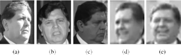
Fig. 5. Sample images from the subset of the LFW dataset. The clipping boxes were painted in red.
Fig. 3. Sample images from the AR dataset.
datasets [38], i.e., LFW deep funneled images [39], [40] and the IJB-A dataset [41]. The ORL dataset contains 400 face images of 40 subjects (10 images per subject) with variations in pose, illumination and facial expression. Fig. 2 shows some sample images of the ORL dataset. The AR dataset consists of 3276 frontal face images of 126 individuals. The images have variation, including in expression, illumination, and pose. Some sample images are shown in Fig. 3. The Extended Yale B dataset contains 2414 images of 38 subjects. 64 frontal face images with various illumination conditions for each subject were taken. Fig. 4 shows some sample images in this dataset. The LFW and IJB-A datasets are designed to study the problem of unconstrained face recognition. All the images were collected from the web. LFW contains 13233 images of 5749 people. IJB-A contains 5712 images of 500 subjects. As there are many individuals with only one or several distinct photos in the datasets, SRC-based methods cannot work well if used directly. Therefore, a subset of each dataset was formed by choosing the subjects with enough training images in the experiments. For the LFW dataset, the subjects with more than 20 images (total 62 subjects) were selected to form the experimental subset. Furthermore, to concentrate on the recognition task, the deep funneled images were used. The face area of each image was extracted using a fixed bounding box, where the upper-left and lower-right corners are (70, 55) and (185, 195), respectively. The determination of the bounding box location is according to the positions of 40 randomly selected LFW faces. Fig. 5 shows some sample images and the clipping boxes of the subset of deep funneled LFW. IJB-A is a dataset released by the Intelligence Advanced Research Projects Activity (IARPA). Readers can refer to http://www.nist.gov/itl/iad/ig/facechallenges.cfm for details. IJB-A has full pose variation, so it is more challenging than LFW. According to each split, only the subjects with more than 20 training images (total 51 subjects) were selected to build the experimental subset. Each image was cropped according to the hand-labelled bounding box and resized to the size of 120*150. Fig. 6 shows some cropped images of the subset of IJB-A.
Fig. 6. Sample cropped images from the subset of the IJB-A dataset.
To demonstrate the superiority of the proposed method, the KLS-GSRC was comprehensively compared with sev- eral related sparse representation based face recognition methods [4], [20], [31], [32]. In addition, two variants of LGSR, named LGSR (with P2) and LGSR (with ker- nel), were also compared. The LGSR (with P2) applies the group sparsity by minimizing the number of nonzero reconstructed vectors instead of the number of nonzero coef- ficients, and the LGSR (with kernel) extends the locality measure from the Euclidian space to the kernel space. Further- more, two non-sparse algorithms, a collaborative representa- tion based method (CRC) [34] and a Matrix Regression based method (NMR) [42] were also compared. CRC represents a test image associated with all the training samples and minimizes the representation error using the least square criterion. NMR is a two-dimensional image-matrix-based error model. Differing from the traditional one-dimensional pixel- based model, it utilizes the two-dimensional structure of the error image to enhance classification performance.
A.Parameter Settings
ε = 0.05, η = 0.25 throughout the experiments. Prin- cipal component analysis (PCA) [43] was used to reduce feature dimension before classification. To choose the value of λ, the performance of KLS-GSRC on three datasets was investigated by varying λ in the range of 0.00001, 0.0001, 0.001, 0.01, 0.1, 1, 1.5. For each test, half of the images were randomly selected as the training set, and the remainder as the test set. The experimental results are reported in Table I. It shows that λ = 0.0001 consistently yields the best results in the three datasets, and this setting is used in the following experiments.
TABLE I
PERFORMANCE UNDER DIFFERENT PARAMETER VALUES OF λ ON THREE
DATASETS
TABLE III
PERFORMANCE OF DIFFERENT METHODS ON THE AR DATASET
TABLE II
PERFORMANCE UNDER DIFFERENT TRAINING/TEST SPLIT SETTINGS ON THE
ORL DATASET
B.Results on ORL Database
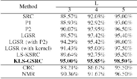
In this experiment, the performance of different methods under different training/test split settings on the ORL dataset were evaluated. For each test, a subset with L (L = 3, 4, 5) images per subject was randomly seleced to form the training set, and the remaining images were taken as the testing set. The recognition accuracy was computed by averaging over 30 independent tests. To make a fair comparison, the high- est average recognition rate of each method under different parameter settings was recorded, as seen in Table II.
As shown in Table II, the highest recognition ratio was consistently obtained by the proposed method under different training/test split settings. The superiority of minimizing the number of nonzero reconstructed vectors instead of the number of nonzero coefficients can be verified by comparing the performance of P1 and P2. The same conclusion can be drawn by comparing LGSR and LGSR (with P2). When the kernelized locality-sensitive constraint is imposed, LS-KSRC can obtain an improvement of about 1% over SRC.
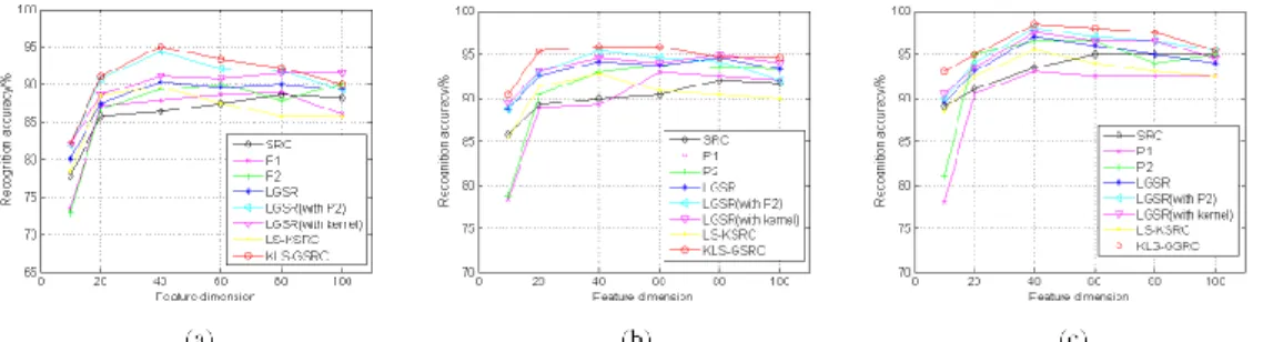
Fig. 7 shows the recognition ratio of different methods under different feature dimension and training/testing split settings. It can be seen that the method always outperforms the others with only one exception (L = 3, feature dimension = 100). The best performance is obtained when the training percentage is 50% (Fig. 7(c)) and the PCA dimension is 40. This method reaches the highest recognition rate of 98.50%, which is at least 0.5% higher than the other methods.
C. Experiments on AR Database
In these experiments, a subset of the AR dataset with pic- tures of 50 males and 50 females was considered. All images were cropped to 165*120 pixels. In each test, 7 images per
subject were randomly selected to form the training dataset, and the rest were used as the test dataset. Table III shows the average recognition rate of different methods under different PCA dimension reduction settings.
In Table III, the method shows its superiority over other methods under different PCA dimension reduction settings. When the feature dimension is 36, the method can achieves a 5.00% performance improvement over LGSR, 1.85% over LGSR (with P2), 3.71% over LGSR (with kernel), and a 6.72% improvement over LS-KSRC.
D. Experiments on Extended Yale B Database
In this experiment, a subset with 32 images per individual was selected for training, and the remaining images were used for testing. Table IV gives the average recognition accuracy of different methods under different PCA dimension reduction settings.
As shown in Table IV, the proposed method still out- performs others methods. The KLS-GSRC obtains the high- est recognition ratio (97.17%) under feature dimension 504. When the feature dimension was reduced to 36, the method obtained the best recognition performance with an accuracy of 92.18%. This performance is about 9.72% higher than P2, 3.65% higher than LGSR, 2.14% higher than LGSR (with P2) method, 1.37% higher than LGSR (with kernel) and 3.95% higher than LS-KSRC. This result is consistent with the previous experimental results on the others datasets. Notably, the integration of kernelized locality-sensitive and group sparsity constraint can achieve better performance than applying them individually. This verifies that the embedded structure information can be better explored by combining these two constraints.
E.Experiments on a Subset of LFW Deep Funneled Images Since the image numbers of individuals in the LFW dataset are different, in this experiment, 50% of images of each individual were selected for training, and the remaining images were used for testing. There were 1526 images for training and 1497 images for testing. Table V gives the average recognition accuracy of different methods under different PCA dimension reduction settings.
As shown in Table V, the performance of the SR-based methods declined in the unconstrained dataset because the
Fig. 7. Performance under different feature dimension settings on the ORL dataset. (a) L = 3. (b) L = 4. (c) L = 5.
TABLE IV
PERFORMANCE OF DIFFERENT METHODS ON THE EXTENDED YALE B DATASET
TABLE VI
PERFORMANCE OF DIFFERENT METHODS ON THE SUBSET OF IJB-A DATASET
TABLE V
TABLE VII
PERFORMANCE OF THE PROPOSED METHOD ON THE SUBSET OF IJB-A DATASET
WITH DIFFERENT ε (PCA DIMENSION IS FIXED TO 300) PERFORMANCE OF DIFFERENT METHODS ON THE SUBSET OF DEEP FUN-
NELED LFW DATASET
significant variation of the images of each individual leads to significant regression error. However, the proposed method still outperforms other methods.
F.Experiments on a Subset of IJB-A Cropped Images The gallery images of each split were used as training samples and the probe images as test images. Table VI reports the average recognition accuracy of different methods under different PCA dimension reduction settings.
The performances of the SR-based methods on IJB-A are worse than on LFW due to the bigger pose variation in IJB-A. The group constraint is also affected by the big pose variation so that the performance of the proposed method is slightly lower than of SRC and LS-KSRC.
G. Experiments about Sparsity
It can be seen from the above experiments that the CRC method achieves comparable performance on three canonical datasets but achieves poor performance on two unconstrained
datasets. In the unconstrained case, many images of other individuals may be more similar than those of the same indi- vidual. Discrimination ability of CR is reduced by regression error. It can be seen that the sparsity constraint effectively improves the recognition performance (more than 25%) in the unconstrained case.
When the sparse coefficient vectors in each method are analyzed, it is found that the sparsity of SRC, LS-KSRC and KLS-GSRC is better than that of P1 (each test image is represented with less than 10% of samples) and LGSR (each test image is represented with most of the samples). Therefore, the experimental results of those methods verify that sparsity improves the face recognition performance.
The method on IJB-A with different ε was evaluated. The results are shown in Table VII. The sparsity is defined as the average number of samples with a coefficient less than 1e-5. It can be seen that the performance improves with the increase of sparsity, and the best performance is achieved at a specific sparsity.
V. CONCLUSION
This paper presents a kernelized locality-sensitive group sparsity representation (KLS-GSRC) method for robust face recognition. KLS-GSRC not only takes into account the grouped structure information of the training dictionary, but also considers the data locality in the kernel space. As a
result, the structure and nonlinear information embedded in the training and test data can be better utilized, and more discriminative sparse representation can be obtained. These experiments on the ORL, AR, Extended Yale B and LFW datasets demonstrated the proposed joint sparse representation method achieves better performance than other sparse repre- sentation based methods.
REFERENCES
[1] Y. Su, S. Shan, X. Chen, and W. Gao, “Hierarchical ensemble of global and local classifiers for face recognition,” IEEE Trans. Image Process., vol. 18, no. 8, pp. 1885–1896, Aug. 2009.
[2] W. Ou, X. You, D. Tao, P. Zhang, Y. Tang, and Z. Zhu, “Robust face recognition via occlusion dictionary learning,” Pattern Recognit., vol. 47, no. 4, pp. 1559–1572, 2014.
[3] S. Xie, S. Shan, X. Chen, and J. Chen, “Fusing local patterns of Gabor magnitude and phase for face recognition,” IEEE Trans. Image Process., vol. 19, no. 5, pp. 1349–1361, May 2010.
[4] J. Wright, A. Y. Yang, A. Ganesh, S. S. Sastry, and Y. Ma, “Robust face recognition via sparse representation,” IEEE Trans. Pattern Anal. Mach. Intell., vol. 31, no. 2, pp. 210–227, Feb. 2009.
[5] X. Chai, S. Shan, X. Chen, and W. Gao, “Locally linear regression for pose-invariant face recognition,” IEEE Trans. Image Process., vol. 16, no. 7, pp. 1716–1725, Jul. 2007.
[6] A. Wagner, J. Wright, A. Ganesh, Z. Zhou, H. Mobahi, and Y. Ma, “Toward a practical face recognition system: Robust alignment and illumination by sparse representation,” IEEE Trans. Pattern Anal. Mach. Intell., vol. 34, no. 2, pp. 372–386, Feb. 2012.
[7] Y. Xu et al., “Data uncertainty in face recognition,” IEEE Trans. Cybern., vol. 44, no. 10, pp. 1950–1961, Oct. 2014.
[8] D. L. Donoho, “Compressed sensing,” IEEE Trans. Inf. Theory, vol. 52, no. 4, pp. 1289–1306, Apr. 2006.
[9] E. J. Candès and M. B. Wakin, “An introduction to compressive sampling,” IEEE Signal Process. Mag., vol. 25, no. 2, pp. 21–30, Mar. 2008.
[10] K. Huang and S. Aviyente, “Sparse representation for signal classifica- tion,” in Proc. NIPS, vol. 19. 2006, pp. 609–616.
[11] W. Liu, Z.-J. Zha, Y. Wang, K. Lu, and D. Tao, “ p-Laplacian regular- ized sparse coding for human activity recognition,” IEEE Trans. Ind. Electron., vol. 63, no. 8, pp. 5120–5129, Aug. 2016.
[12] J. Yang, J. Wright, T. S. Huang, and Y. Ma, “Image super-resolution via sparse representation,” IEEE Trans. Image Process., vol. 19, no. 11, pp. 2861–2873, Nov. 2010.
[13] J. Wright, Y. Ma, J. Mairal, G. Sapiro, T. S. Huang, and S. Yan, “Sparse representation for computer vision and pattern recognition,” Proc. IEEE, vol. 98, no. 6, pp. 1031–1044, Jun. 2010.
[14] R. Zhi, M. Flierl, Q. Ruan, and W. B. Kleijn, “Graph-preserving sparse nonnegative matrix factorization with application to facial expression recognition,” IEEE Trans. Syst., Man, Cybern. B, Cybern., vol. 41, no. 1, pp. 38–52, Feb. 2011.
[15] S. Zhang, H. Yao, X. Sun, and X. Lu, “Sparse coding based visual tracking: Review and experimental comparison,” Pattern Recognit., vol. 46, no. 7, pp. 1772–1788, Jul. 2013.
[16] D. Wang, H. Lu, and M.-H. Yang, “Online object tracking with sparse prototypes,” IEEE Trans. Image Process., vol. 22, no. 1, pp. 314–325, Jan. 2013.
[17] M. Yang and L. Zhang, “Gabor feature based sparse representation for face recognition with Gabor occlusion dictionary,” in Proc. ECCV, 2010, pp. 448–461.
[18] W. Deng, J. Hu, and J. Guo, “Extended SRC: Undersampled face recognition via intraclass variant dictionary,” IEEE Trans. Pattern Anal. Mach. Intell., vol. 34, no. 9, pp. 1864–1870, Sep. 2012.
[19] M. Yuan and Y. Lin, “Model selection and estimation in regression with grouped variables,” J. Roy. Statist. Soc. B, Statist. Methodol., vol. 68, no. 1, pp. 49–67, 2006.
[20] E. Elhamifar and R. Vidal, “Robust classification using structured sparse representation,” in Proc. CVPR, 2011, pp. 1873–1879.
[21] J. Lai and X. Jiang, “Classwise sparse and collaborative patch represen- tation for face recognition,” IEEE Trans. Image Process., vol. 25, no. 7, pp. 3261–3272, Jul. 2016.
[22] X. Jiang and J. Lai, “Sparse and dense hybrid representation via dictionary decomposition for face recognition,” IEEE Trans. Pattern Anal. Mach. Intell., vol. 37, no. 5, pp. 1067–1079, May 2015.
[23] K.-R. Müller, S. Mika, G. Rätsch, K. Tsuda, and B. Schölkopf, “An introduction to kernel-based learning algorithms,” in Handbook of Neural Network Signal Processing. Boca Raton, FL, USA: CRC Press, 2001.
[24] H. Van Nguyen, V. M. Patel, N. M. Nasrabadi, and R. Chellappa, “Kernel dictionary learning,” in Proc. ICASSP, 2012, pp. 2021–2024.
[25] L. Zhang et al., “Kernel sparse representation-based classifier,” IEEE Trans. Signal Process., vol. 60, no. 4, pp. 1684–1695, Apr. 2012. [26] S. Gao, I. W.-H. Tsang, and L.-T. Chia, “Sparse representation with
kernels,” IEEE Trans. Image Process., vol. 22, no. 2, pp. 423–434, Feb. 2013.
[27] A. Shrivastava, V. M. Patel, and R. Chellappa, “Multiple kernel learn- ing for sparse representation-based classification,” IEEE Trans. Image Process., vol. 23, no. 7, pp. 3013–3024, Jul. 2014.
[28] K. Yu, T. Zhang, and Y. Gong, “Nonlinear learning using local coordi- nate coding,” in Proc. NIPS, 2009, pp. 2223–2231.
[29] J. Wang, J. Yang, K. Yu, F. Lv, T. Huang, and Y. Gong, “Locality- constrained linear coding for image classification,” in Proc. CVPR, 2010, pp. 3360–3367.
[30] J. Tang, L. Shao, and X. Li, “Efficient dictionary learning for visual categorization,” Comput. Vis. Image Understand., vol. 124, pp. 91–98, Jul. 2014.
[31] Y.-W. Chao, Y.-R. Yeh, Y.-W. Chen, Y.-J. Lee, and Y.-C. F. Wang, “Locality-constrained group sparse representation for robust face recog- nition,” in Proc. ICIP, 2011, pp. 761–764.
[32] S. Zhang and X. Zhao, “Locality-sensitive kernel sparse representation classification for face recognition,” J. Vis. Commun. Image Represent., vol. 25, no. 8, pp. 1878–1885, 2014.
[33] E. Grave, G. R. Obozinski, and F. R. Bach, “Trace Lasso: A trace norm regularization for correlated designs,” in Proc. NIPS, 2011, pp. 2187–2195.
[34] L. Zhang, M. Yang, and X. Feng, “Sparse representation or collaborative representation: Which helps face recognition?” in Proc. ICCV, 2011, pp. 471–478.
[35] F. S. Samaria and A. C. Harter, “Parameterisation of a stochastic model for human face identification,” in Proc. IEEE Workshop Appl. Comput. Vis., Dec. 1994, pp. 138–142.
[36] A. M. Martinez, “The AR face database,” CVC, Barcelona, Spain, Tech. Rep. #24, 1998.
[37] A. S. Georghiades, P. N. Belhumeur, and D. Kriegman, “From few to many: Illumination cone models for face recognition under variable lighting and pose,” IEEE Trans. Pattern Anal. Mach. Intell., vol. 23, no. 6, pp. 643–660, Jun. 2001.
[38] C. Ding and D. Tao, “A comprehensive survey on pose-invariant face recognition,” ACM Trans. Intell. Syst. Technol., vol. 7, no. 3, p. 37, 2016. [39] G. B. Huang, M. Ramesh, T. Berg, and E. Learned-Miller, “Labeled
faces in the wild: A database for studying face recognition in uncon- strained environments,” Univ. Massachusetts, Amherst, MA, USA, Tech. Rep. 07-49, 2007.
[40] G. Huang, M. Mattar, H. Lee, and E. G. Learned-Miller, “Learning to align from scratch,” in Proc. NIPS, 2012, pp. 764–772.
[41] B. F. Klare et al., “Pushing the frontiers of unconstrained face detection and recognition: IARPA Janus benchmark A,” in Proc. CVPR, 2015, pp. 1931–1939.
[42] J. Yang, L. Luo, J. Qian, Y. Tai, F. Zhang, and Y. Xu, “Nuclear norm based matrix regression with applications to face recognition with occlusion and illumination changes,” IEEE Trans. Pattern Anal. Mach. Intell., vol. 39, no. 1, pp. 156–171, Jan. 2017.
[43] S. Wold, K. Esbensen, and P. Geladi, “Principal component analysis,” Chemometrics Intell. Lab. Syst., vol. 2, nos. 1–3, pp. 37–52, Jan. 1987.
Shoubiao Tan received the Ph.D. degree from the
University of Science and Technology of China, in 2004. He is currently a Professor with Anhui Uni- versity, China. His current research interests include computer vision and pattern recognition.
Xi Sun received the M.Eng. degree from Anhui University in 2016. She is currently a Lecturer with the Anhui Post and Telecommunications College, China. Her research interests include information processing and face recognition.
Lei Qu received the Ph.D. degree from Anhui
University, China, in 2008. He has conducted Post- Doctoral research work with the Janelia Farm Research Campus, Howard Hughes Medical Insti- tute, from 2009 to 2011. He is currently a Professor with Anhui University. His current research inter- ests include computer vision and biological image processing.
Wentao Chan is currently pursuing the master’s
degree with the School of Electronics and Infor- mation Engineering, Anhui University, China. His research interests include computer vision and face recognition.
Ling Shao received the B.Eng. degree in electronic
and information engineering from the University of Science and Technology of China, and the M.Sc. degree in medical image analysis and the Ph.D. degree in computer vision from the University of Oxford. He is currently a Professor with the School of Computing Sciences, University of East Anglia, Norwich, U.K. He has authored or co-authored over 200 papers in refereed journals/conferences, such as the IEEE TPAMI, TIP, TNNLS, IJCV, ICCV, CVPR, ECCV, IJCAI and ACM MM, and holds over 10 EU/US patents. His current research interests include computer vision, image/video processing, pattern recognition and machine learning. He is a fellow of the British Computer Society, the IET, and a Life Member of the ACM.