Comparative Vigilance
Brown University Department of Economics Working Paper No. 2008-9 Allan M. Feldman
Department of Economics, Brown University Providence, RI 02906 USA
http://www.econ.brown.edu/fac/allan_feldman
Ram Singh
Department of Economics Delhi School of Economics
University of Delhi Delhi 110007, India [email protected] http:www.econdse.org/faculty-frame.htm June 5, 2008 Abstract
A growing body of literature suggests that courts and juries are inclined toward division of liability between two strictly non-negligent or “vigilant” parties. However, standard models of liability rules do not provide for vigilance-based sharing of liability. In this paper, we explore the economic efficiency of liability rules based on comparative vigilance. We devise liability rules that are efficient and that reward vigilance exhibited by the parties. It is commonly believed that discontinuous liability shares are necessary for efficiency, but we develop a liability rule that is both efficient and continuous, based on comparative negligence when both parties are negligent and on comparative vigilance when both parties are vigilant. Moreover, our rule divides accident losses into two parts: one part creates incentives for efficiency; the other part provides equity.
Keywords: Comparative vigilance, equity, economic efficiency, tort liability rules, Nash
equilibrium, social costs, pure comparative vigilance, super-symmetric rule
1 INTRODUCTION
Tort liability rules determine how accident losses resulting from risky activities are borne by the parties involved. The economic analysis of liability rules has typically considered accidents resulting from the activities of two parties. This analysis has led to characterizing some rules as efficient and others as inefficient. Models used in economic analysis have imposed certain conditions on the structure of liability rules, some of which vary from rule to rule, some of which do not. The rules that have been proven to be efficient generally satisfy the following three conditions:
(A) When one party is negligent and the other is not, the negligent party bears all the accident loss;
(B) When both parties are non-negligent, the liability shares do not depend on the degrees of “vigilance” shown by the parties, that is, the care levels above and beyond what is efficient.
(C) When both parties are non-negligent, all the accident loss falls on just one party.1 While mainstream economic analysis continues to rely on these three conditions, they have been criticized by legal scholars. In this paper, we analyze the implications of relaxing these conditions.
We are motivated by the work of several scholars, including Justice Guido Calebresi, and by some court decisions. Various authors have criticized conditions B and C above.2
Condition C says that when both parties are non-negligent, one and only one party is liable for the entire loss; which party it is depends on the rule in force.3 Calabresi and Cooper (1996) and Parisi and Fon (2004) have argued that when parties are either both negligent, or both non-negligent, equity considerations demand sharing of liability - making only one party bear all
1 See the modeling of liability rules in Brown (1973), Diamond (1974), Polinsky (1989), Landes and Posner
(1987), Shavell (1987), Barnes and Stout (1992), Posner (1992), Levmore (1994), Kaplow (1995), Biggar (1995), Miceli (1997), Cooter and Ulen (1997), Feldman and Frost (1998), Jain and Singh (2002), Kim (2004), Kim and Feldman (2006), and Singh (2007), among others.
2 For criticism of the modeling of liability rules on various grounds including these two assumptions, see Grady
(1989), Kahan (1989), Marks (1994), Burrow (1999) and Wright (2002).
3 This party is the victim under the rules of negligence, negligence with a defense of contributory negligence,
negligence with a defense of comparative negligence. Under the rule of strict liability with a defense of contributory negligence, however, the injurer bears the entire loss.
the loss is not justified. Calabresi and Cooper (1996) and Honoré (1997) have recommended proportionate or comparative apportionment of accident losses in such instances.4 These scholars have argued that judicial decision making is influenced by equity considerations. Moreover, some studies have shown that courts and juries are inclined toward comparative apportionment of losses when both parties are negligent and when both are non-negligent.
This phenomenon has been observed in several countries, including France, Germany, Japan and U.S. (See Calabresi and Cooper (1996), Yoshihsa (1999), Grimley (2000), Yu (2000) and Parisi and Fon (2004).) In India, special legislation requires sharing of certain types of
accident losses, when both injurer and victim are non-negligent.5
Condition A requires that all the loss fall on the negligent party when one party is negligent and the other is not. Kahan (1989) and Honoré (1997) have argued that this is not consistent with the doctrine of “causation.” (Also see Singh (2007).). Under a standard
liability rule like simple negligence, condition A implies that for at least one party, the liability share jumps abruptly from zero to one hundred percent, as that party goes from just meeting his standard of care, to just falling short of meeting that standard.6 Kahan (1989) and Grady (1989), though on different grounds, have argued that this striking discontinuity is not part of the functioning of the law of torts.7
In short, there is a body of literature arguing that some of the basic assumptions of economic models are neither desirable nor in keeping with the reality of judicial decision making. Nonetheless, the usual economic modeling of liability rules continues to incorporate conditions A, B and C. The widespread use of these conditions is not surprising, because they have helped us to make precise and robust statements about the characteristics of various liability rules, including their efficiency properties. Parisi and Fon (2004) have remarked that the discontinuity in liability shares (implied by condition A) provides strong incentives for the
4 Only rule that allows loss sharing is the rule of comparative negligence. However, under this rule, loss sharing
takes place only when both parties are negligent; not when both parties are non-negligent. For an analysis of this rule see Schwartz, (1978), Landes and Posner (1980), Cooter and Ulen (1986), Haddock and Curran (1985), Rubinfeld (1987), and Rea (1987). For a critical review of some of these works see Liao and White (2002), and Bar-Gill and Ben-Shahar (2003).
5 Sections 140 and 163 A of Motor Vehicle Act (1988) require that in instances of death and physical injuries, the
victim be partially compensated if both parties were non-negligent.
6 Note that if the victim is non-negligent, under the rules of negligence, negligence with a defense of contributory
negligence and negligence with a defense of comparative negligence, the injurer’s liability jumps from nil (when he is non-negligent) to full liability (when he is negligent). Similarly, under the rule of strict liability with a defense of contributory negligence, there is drastic jump in the victim’s liability.
parties to opt for efficient care levels. Jain and Singh (2002), Kim (2004), and Singh (2006) have shown that these 3 conditions play a large role in efficiency analysis. But, as we shall see below, the conditions can be relaxed along the lines suggested by legal scholars, without sacrificing efficiency.
In this paper we will develop liability rules that are ‘equitable’ as well as efficient. When both parties are negligent (that is, taking less than the efficient amount of care), one party’s degree of negligence is defined by her shortfall in care divided by the combined
shortfalls in care of the two parties. We think that when both parties are negligent, an equitable liability rule should have liability shares that are generally increasing with degrees of
negligence. When both parties are non-negligent (taking at least the efficient amount of care)
and at least one is vigilant (taking more than the efficient amount of care), each party’s degree of vigilance can be defined as her excess of care divided by the combined excesses of care of the two parties. We think that when both parties are vigilant, an equitable liability rule should have liability shares that are generally decreasing with degrees of vigilance. We also believe
liability shares should vary continuously over all possible combinations of care levels. And, of course, we want our rules to result in efficient outcomes. That is, social-cost-minimizing care levels for the 2 parties should always be Nash equilibria, and there shouldn’t be other
(inefficient) Nash equilibria.
In section 2 of this paper we lay out our model and most of our definitions. In section 3 we briefly discuss pure comparative negligence, which, when both parties are negligent, makes each party’s liability share equal to her degree of negligence. As is well known, under pure comparative negligence the efficient combination of care levels of the two parties is a Nash equilibrium (theorem 1) and there are no other Nash equilibria (theorem 2). We then turn to a rule which closely parallels pure comparative negligence, but which is defined when both parties are non-negligent and at least one is vigilant. This is pure comparative vigilance; it makes each party’s liability share equal to 1 minus her degree of vigilance. Pure comparative vigilance and its relatives discussed in section 3 depart from conditions B and C above. We show that the efficient pair of care levels is not a Nash equilibrium under pure comparative
vigilance (theorem 3), and we construct an example to show that under pure comparative vigilance, there may be inefficient Nash equilibria which involve both parties taking too much care.
The negative results for pure comparative vigilance are interesting when compared with the efficiency results (theorems 1 and 2) for pure comparative negligence. Under both pure comparative vigilance and pure comparative negligence, by increasing her care a party
unilaterally reduces her liability share. Why does this result in efficiency for pure comparative negligence but inefficiency for pure comparative vigilance? The explanation is quite simple: when both parties are negligent, the “equity” consideration (reward more care) and the
efficiency consideration (efficiency requires more care by both parties) are aligned. In contrast, when both parties are taking too much care, under pure comparative vigilance, the “equity” consideration (reward more care) and the efficiency consideration (the parties are already taking too much care) are opposed.
We then turn to modified versions of comparative vigilance. We construct a rule that is analogous to comparative negligence with fixed division, and we show (theorems 4 and 5) that our rule of comparative vigilance with fixed division has the desired efficiency properties.
Comparative vigilance with fixed division departs from condition C above. Next we turn to variants of comparative vigilance which do not involve fixed liability shares, but which achieve efficiency by creating discontinuities on the boundaries of the area where both parties are non-negligent. One such rule creates slices in the surface that represents a party’s liability share, the second shifts entire parts of that surface. We establish efficiency results in theorems 6 and 7 (for the sliced surface rule) and theorems 8 and 9 (for the shifted surface rule).
The fixed-division comparative vigilance rule, as well as the sliced and shifted versions of comparative vigilance, all have undesirable discontinuities. (In this respect they are like the traditional rules of negligence, negligence with comparative negligence, and so on.) In section 4 of the paper we develop a new rule which (1) has liability shares that are continuous over all combinations of care levels, (2) is based on the idea of comparative negligence when both parties are negligent and on the idea of comparative vigilance when both parties are vigilant, (3) treats comparative negligence and comparative vigilance symmetrically, and (4) allows increased care to reduce liability shares even when one party is negligent and the other party is non-negligent. This rule departs from all three of the traditional conditions A, B and C. And yet, this rule is efficient: the efficient care combination is a Nash equilibrium (theorem 11), and there is no Nash equilibrium in the region where both parties take too much care (theorem
10) or too little care (theorem 12). We call this new rule the “super-symmetric comparative negligence and vigilance rule,” or the “super-symmetric” rule for short.
Mainstream economic models of liability rules require sharp discontinuities in liability share; our super-symmetric rule does not. Mainstream models lean on conditions A, B and C; our super-symmetric rule drops all three. Finally, our super-symmetric rule has one more feature that sets it off: Standard tort liability rules allocate total expected accident costs
between the two parties. Our super-symmetric rule divides expected accident costs into two parts: a fixed component equal to the party’s expected costs at the efficient care point, and a variable component equal to the rest. Our liability rule apportions only the variable
component according to comparative negligence, comparative vigilance, and so on. This is the mathematical key to several of our results.
.
2 DICHOTOMOUS AND MIXED LIABILITY RULES
Model Preliminaries
We assume there are two risk-neutral people, X and Y, who engage in some activity that creates
a risk of accidents. An accident is an unintended and unforeseen bad outcome. If an accident occurs, there is one victim, who sustains a monetary loss , and one injurer, who sustains no loss. We assume that X is the injurer and Y is the victim. For simplicity, the loss
0
> L
L is assumed to be constant.
Let x and y denote person X’s and person Y’s care levels, respectively, measured by
their care expenditures. Following the standard modeling in tort liability literature since Brown (1973), we assume that each person can choose any level of care between 0 and ∞, and that the probability of an accident, p(x,y), is a continuous and differentiable function of x
and . We assume that increasing care levels reduce the probability of an accident, and thus expected accident costs ( , and
y
0
<
x
p py <0). We also assume that, for all x and y,
, , , and . 0 ) , (x y > p pxx >0 pyy >0 pxy >0
When we need to work with an example of an accident probability function, we will use the following:
1 1
( , ) (1 ) (1 )
2 1 (1 ) (1 ) (1 ) x p p x y x − − − = − + + = + , 1 2 (1 ) (1 ) (1 ) y p p x y y − − − = − + + = + 3 1 2(1 ) (1 ) xx p = +x − +y − , pyy =2(1+x) (1−1 +y)−3 2 2 (1 ) (1 ) xy yx p = p = +x − +y −
Total social cost (TSC) is defined as the sum of care-taking costs of both parties and
expected accident costs. That is, TSC= + +x y p x y L( , ) . The social goal is, as usual, to
minimize total social cost. Let denote the solution to this TSC minimization problem.
We will assume for the sake of clarity in this paper that ( ) is unique. We call the efficient care combination.
) , ( * * y x * *, y x (x*,y*)
Negligence-Based Liability Rules
In this model, when an accident occurs the entire loss L is initially born by the victim Y. The
court then enforces a liability rule, which determines where L ultimately falls: on the victim, on the injurer, or on both according to some mixing rule. A negligence-based liability rule is defined in terms of which parties are negligent. If both are negligent, it may be defined in terms of the degree to which they are negligent; if both are non-negligent, it may be defined in terms of the degree to which they are non-negligent. A party is negligent if her care
expenditure is less than the court-enforced standard of care. A party is non-negligent if her
care expenditure is greater than or equal to the standard of care. A party is strictly non-negligent, or vigilant, if her care expenditure is greater than the standard of care. We assume
that everyone, including the court, knows the expected loss function and the governing liability rule, that the court can solve the TSC minimization problem, and that everyone, including the
court, can observe each party’s care level accurately.
Finally, we assume that the standard of care for each party is set at the efficient level. That is, for instance, party X is found negligent by the court if and only if she spends .
This is an especially basic assumption, and we will use it throughout this paper. We call it: *
x x<
Axiom 1: The court sets the standards of care at the efficient levels ( ). That is,
party X (or Y) is negligent if and only if (or ).
* *, y x * x x< y< y*
For the related terminology: Party X (or Y) is non-negligent if x*≤x (ory*≤ y). Party X (or Y) is strictly non-negligent, or vigilant, if x* <x (ory*< y).
Typically, legal rules only allow a court to distribute the loss L between the two parties,
that is, to assign each party a fraction of the loss, greater than or equal to zero, with the two fractions summing to one. Such rules will be called normal. With a normal rule, a party in a lawsuit ends up with some loss between 0 and L, and the sum of the losses falling on the two
parties equals L. Non-normal rules allow the fractions falling on the two parties to be negative
or greater than one (e.g., punitive damages), or to sum to numbers other than one (e.g., with the rest of society picking up some of the losses; or with both parties paying L, the “both pay full
costs” rule).
Formally, a normal negligence-based liability rule examines the actual behavior of both
parties, plus the efficient behavior of both parties, plus L, plus the probability function ,
and then enforces a normal loss allocation of the accident loss L between the parties. A normal loss allocation is a vector of weights , where
) , (x y p ) , (wX wY 0≤wX,wY ≤1, wX +wY =1, = the
fraction of the loss the liability rule places on party X, and = the fraction of the loss the
liability rule places on party Y. In this paper we will only consider normal liability rules.
X
w
Y
w
Negligence-based liability rules are usually defined by specifying how they operate in 4 different domains: Domain 1, where both parties are non-negligent; domain 2, where party X
is negligent and party Y is non-negligent; domain 3, where both parties are negligent; and domain 4, where party Y is negligent and party X is non-negligent. (See figure 1 below.) We
will sometimes lump domains 2 and 4 together, and describe them jointly as the one-party-negligent, one-party-non-negligent region. Because X is non-negligent if and only ifx* ≤x, and similarly for Y, domain 1 is the set {( , )x y x*≤x&y* ≤y}. It will sometimes be necessary to partition this set into the point ( , )* *
x y , and the rest (where at least one person is strictly
non-negligent, or vigilant). Domain 2 is the set {( , ) *& * }
x y x<x y ≤ y (that is, X negligent
and Y non-negligent), and domain 4 is {( , )x y x*≤x&y< y*} (that is, X non-negligent and Y
negligent). Domain 3 is the set {( , ) *& *}
in a domain if it places all costs on just one party in that domain. We call a liability rule dichotomous if it is dichotomous in all 4 domains. For a normal dichotomous liability rule in a
domain, must equal either or . For example, the familiar real world negligence-based liability rules are dichotomous in domains 2 and 4, where one and only one party is negligent; and they place all the losses on the negligent party in those domains. (This is condition A from section 1.) Such rules include simple negligence, negligence with a
defense of contributory negligence, negligence with a defense of comparative negligence, strict liability with a defense of contributory negligence, and so on.
) ,
(wX wY (0,1) (1,0)
INSERT FIGURE 1 HERE
We now restate condition A from section 1, and we will call it an axiom here because of its importance in the real world. We use this assumption in section 3 of this paper, but we will drop it in section 4, when we develop our super-symmetric rule.
Axiom 2: In domains 2 and 4, all losses fall on the negligent party. That is, if *& *
x<x y ≤y, then (wX,wY) (1,0)= , and if x*≤x&y< y*, then (wX,wY) (0,1)= .
In domain 1, where both parties are non-negligent, the real world liability rules are dichotomous; that is they place all the losses on just one party. Moreover, that party remains fixed, no matter what the degrees of vigilance of the two parties might be. The following axiom formalizes this idea, and is both simpler and logically stronger than the related
conditions B and C from section 1 above. Although axiom 3 (in combination with axioms 1 and 2) has played an important role in efficiency characterizations of liability rules in the literature (see Jain and Singh (2002)), we will drop it throughout this paper.
Axiom 3: In domain 1, either (wX,wY) (1,0)= for all x*≤x& y*≤ y, or (wX,wY) (0,1= ) for all x*≤x& y*≤ y.
We call a liability rule mixed in a domain if it places non-zero costs on both parties at some
points in that domain. For example, pure comparative negligence is mixed in the both parties negligent domain, i.e., domain 3. We call a liability rule mixed if it is mixed in at least one
domain.
We use the following convenient notation throughout this paper: For any x and any ,
let y * x x x Δ = − and * y y y
Δ = − . Note that Δx (or Δy) can be positive, zero, or negative, depending on whether X (or Y) is vigilant, is at the optimum care level, or is negligent,
respectively.
First, suppose both parties are negligent (domain 3). If both parties are negligent,
then * 0 and . Note that
x x x
Δ = − < * 0
y y y
Δ = − < *
x − = −Δx x is the dollar measure of party X’s shortfall from her proper (efficient) degree of care, and similarly with −Δy and party
Y. The most natural way to define party X’s relative degree of negligence, or degree of fault, is
set it equal to the ratio of X’s shortfall in care to the sum of the shortfalls of the two parties.
That is, X’s degree of negligence (or degree of fault) is * * * x x x x x x y y x y x y − −Δ Δ = = − + − −Δ − Δ Δ + Δ .
Similarly, party Y’s degree of negligence (or degree of fault) is * * * y y y x x y y x y − Δ = − + − Δ + Δ .
Under a pure comparative negligence liability rule, the fractional parts of losses that fall on the
respective parties are set equal to these respective factors. That is, X
x w x y Δ = Δ + Δ and Y y w x y Δ = Δ + Δ .
Note the following about this loss allocation rule: For a fixed 0 * y y
< − , consider party
X’s loss share wX. It is greatest when x=0, and it declines monotonically as from
below, approaching a limit of 0. Note that and are not defined at the point ; nor are the limits defined as ( ,
* x x→ X w wY ) , ( ) , ( * * y x y x = x y) approaches ( , )x y* * .
Figure 2 below illustrates wX in the both parties negligent domain (domain 3).
Second, suppose both parties are non-negligent (domain 1). Then 0≤ −x x* = Δx and
*
0≤ −y y = Δy. Can we define a mixed liability rule in this domain, with the same logic as is
used for the rule of pure comparative negligence in the both parties negligent domain?
For this purpose we will require that at least one of the inequalities be strong, in order to avoid having a zero in the denominator of a fraction. That is, for the purposes of this
discussion, we are assuming ( , )x y is in {( , )x y x*≤x&y*≤ y} \ ( , )x y* * . At least one party is strictly non-negligent, or vigilant.
In the analysis of pure comparative negligence, party X’s degree of negligence is defined
as her shortfall in care divided by the sum of the two parties’ shortfalls in care. Following Calabresi and Cooper (1996) and Parisi and Fon (2004), in the both parties non-negligent
domain, we define party X’s relative degree of vigilance as her excess of care divided by the
sum of the two parties’ excesses of care. That is, party X’s degree of vigilance is * * * x x x x x y y x y − = − + − Δ + Δ Δ
. Similarly, party Y’s degree of vigilance is * * * y y y x x y y x y − = − + − Δ + Δ Δ
. Note that the algebraic expressions for degree of vigilance in domain 1 are identical to the expressions for degree of negligence in domain 3.
In the both parties negligent domain, for the pure comparative negligence liability rule, we let party X’s liability weight equal her degree of negligence. In the both parties
non-negligent domain, we obviously don’t want party X’s liability weight to be equal to her degree
of vigilance; the idea is to reward vigilance rather than punish it. What makes sense is for party X’s vigilance to add to partyY’s liability weight. The straightforward way to do this is to
assume that the fractional part of losses falling on party X equals 1 minus her degree of
vigilance, and similarly for party Y.
X
w
That is, when both parties are negligent (with at least one party strictly non-negligent), X’s share of the loss equals X 1
x y
w
x y x y
Δ Δ
= − =
Δ + Δ Δ + Δ , and Y’s share of the loss
equals Y x w x y Δ =
Δ + Δ . We call a liability rule that uses these weights in domain 1 a pure comparative vigilance rule.
Note the following about this loss allocation rule: For a fixed 0 * y y y
< Δ = − , consider party X’s loss share wX. It declines monotonically as x increases. It approaches a limit of 0
as x→∞. As from above, it approaches a limit of 1. Note that these shares are
defined only in the both parties non-negligent domain, and only if at least one party is strictly non-negligent..
*
x x→
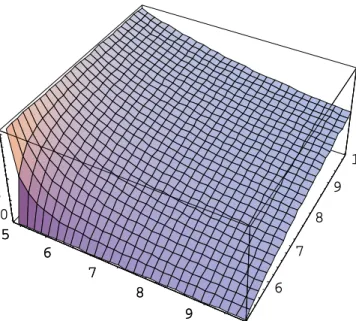
Figure 3 below illustrates the we have just defined in the both parties non-negligent domain (domain 1).
X
w
INSERT FIGURE 3 HERE
It is tempting to define “degree of something” measures that are identical to the degree of negligence and degree of vigilance measures on their domains, but which are defined over all 4 domains. Can this be done? We could use (and ) as defined above on domains 1 and 3, and (following axiom 2) set = 1 when party X is negligent and party Y is non-negligent,
and = 0 when party X is non-negligent and party Y is negligent . This would produce a
function defined over the union of the 4 domains, mixed on the both parties negligent and the both parties non-negligent domains, and dichotomous on the one and only one party negligent domains. (The liability weights would have to be separately defined at the efficient point itself.) This would be a pure comparative negligence and pure comparative vigilance rule,
continuous over the entire quadrant, except at the point
X w wY X w X w wX * *
( , )x y . As we shall see, however,
such a rule would be problematic, because of difficulties with pure comparative vigilance. In much of section 3 below, in order to examine pure comparative vigilance, we will specify the weights in domains 1, 2 and 4, but leave weights in domain 3, where both are negligent, unspecified. In section 4 below, we will define a new rule, over all 4 domains, that incorporates crucial features of both comparative vigilance and comparative negligence.
3 EFFICIENCY AND NASH EQUILIBRIUM
In this section of the paper, but not in section 4 which follows, we will assume axiom 2: When one party is negligent and the other is not, all losses fall on the negligent party.
Preliminaries – Pure Comparative Negligence
In the standard theory of negligence-based liability rules, a rule is characterized by specifying how the accident costs are born in the 4 domains. For instance, the simple negligence rule sets
= 1 if and only if X is negligent. (Remember, X is the injurer.) Therefore
X
w wX =0 if both
are non-negligent; wX =1 when X is negligent and Y is not; wX =0 when Y is negligent and X
is not; and when both are negligent. The rule of negligence with contributory negligence as a defense sets
1 X
w =
0 X
w = if both are non-negligent; when X is negligent and Y is not; when Y is negligent and X is not; and
1 X
w =
0 X
w = wX =0 when both are negligent. The
rule of negligence with comparative negligence as a defense sets if both are non-negligent; when X is negligent and Y is not;
0 X
w =
1 X
w = wX =0 when Y is negligent and X is not;
and wX x
x y Δ =
Δ + Δ (“pure comparative negligence”) when both are negligent.
Once a liability rule is specified, the economist asks whether the rule would induce rational X and Y to end up at the efficient, social-cost-minimizing point . There are
really two parts to this question, the first being: Is a Nash equilibrium under the rule? The second part is: Is it the only Nash equilibrium? Here are the questions and answers for the rule of negligence with a defense of comparative negligence. Since these are well-known results, we omit the proofs:
) , ( * * y x ) , ( * * y x
Theorem 1: is a Nash equilibrium under negligence with a defense of comparative negligence. ) , ( * * y x
Theorem 2: is the only Nash equilibrium under negligence with a defense of comparative negligence. ) , ( * * y x
Pure Comparative Vigilance
Next we turn to pure comparative vigilance. The focus now is on domain 1, where both are non-negligent. This rule sets wX y
x y Δ = Δ + Δ and Y x w x y Δ =
non-negligent and at least one is strictly non-non-negligent, or vigilant. We will assume that wX =wX and wY =wY at the point( , ). Based on axiom 2,
* *
y
x wX =1 when X is negligent and Y is not;
and when wX =0 Y is negligent and X is not.
If we wanted to complete the specification of our liability rule at this point, we would have to indicate what the weights are in domain 3, where both are negligent. But we need not do so at this time. We can get several interesting results without completely specifying the rule.
We start out by asking: Do efficiency theorems like theorems 1 and 2 hold for pure comparative vigilance? The answer, it turns out, is No.
Theorem 3: (x*,y*) is not a Nash equilibrium under pure comparative vigilance. Proof: Suppose y= y*. If X chooses x<x* she is negligent and Y is not; therefore X is liable and pays all the accident costs. Therefore she will want to move to the right,
since she is attempting to minimize 1 ( , )*
x+ p x y L. Once she reaches x=x*, suddenly takes on the value
X
w
X
w . There are two relevant possibilities: 0<wX ≤1, and 0=wX. In the former case, X bears costs x*+w p x y LX ( , )* * at x*. But farther to the right, at
*
x +ε, say, drops to zero under the pure comparative vigilance rule. So X does not
stop at
X
w *
x , she moves instead to x*+ε. Since x*+ε/ 2 is always better than x*+ε, for any ε >0, there is no Nash equilibrium.
In the latter case, party X has no incentive to move. But now consider party Y. At * *
( , )x y , wX =0, and therefore wY =1. Party Y bears costs y*+1 ( , )p x y L* * . If she
increases by y ε, suddenly drops to zero under the pure comparative vigilance rule. Therefore she moves to
Y
w *
y +ε, and once again there is no Nash equilibrium. QED.
The next question is this: is there something like theorem 2 for pure comparative vigilance? Can we rule out inefficient Nash equilibria in the both parties non-negligent domain? We now focus on the part of domain 1 where both are non-negligent and at least one is strictly non-negligent, that is, vigilant. The first thing to note is that no Nash equilibrium could occur where only one party is vigilant; they must both be. For instance, if X is at x>x*
and Y is at y*, then X 0 y w x y Δ =
Δ + Δ = . Then X will want to move to the left, so they could not
be at a Nash equilibrium. Therefore we can confine our search for inefficient Nash equilibria in domain 1 to its interior, where both parties are vigilant. That is, Δ >x 0 and Δ >y 0.
Under pure comparative vigilance, can we show there is no both-parties-vigilant Nash
equilibrium? We have the following conjecture:
Conjecture: Let ( , )x y be any point in the interior of domain 1, with both parties vigilant. Then ( , )x y is not a Nash equilibrium under pure comparative vigilance.
In the appendix we derive restrictive necessary conditions for ( , )x y to be a Nash equilibrium in the interior of domain 1, hoping to show those conditions make for an impossibility (of an inefficient Nash equilibrium). But it turns out there is no impossibility, which we demonstrate in the appendix with:
Counterexample to conjecture: Let the accident probability function be 1
( , ) (1 ) (1 ) 1
p x y = +x − +y − , and let L=216 6= 3. It is then straightforward to show . Consider the both-parties vigilant point
* * 1/ 3 1 6 1 5
x = y =L − = − =
( , ) (6.3646, 6.3646)x y = . We show that ( , )x y satisfies the restrictive necessary
conditions derived in the conjecture. We show that x minimizes the burden on X, given
the choice by Y of y, and vice versa. Therefore ( , )x y is an inefficient, both parties vigilant, Nash equilibrium under pure comparative vigilance.
We will now turn to modified versions of comparative vigilance, which respond to the disappointing results of theorem 3 and the counterexample above.
Comparative Vigilance With Fixed Division
The simplest modification of the comparative vigilance rule is to make it analogous to the rule of comparative negligence with fixed division. In that rule, if both parties are negligent, their weights and are set equal to constant values, no matter what the degrees of negligence. The values might be , in which case we would have the traditional equal
division rule. X w wY 1/ 2 X Y w =w =
Suppose then we are in the both parties non-negligent domain, with at least one party strictly non-negligent, or vigilant. In this case, let wX =wˆX and let , for some constant
, with . At the point
ˆ Y w =wY 1 ≤ ˆ ˆ 0≤wX,wY wˆX +wˆY =1 * *
( , )x y we again assume the weights are wX and wY. Moreover we will require that ˆ(wX,wˆY) (= wX,wY). Following are the results that
Before proceeding, we need to introduce some notation for the part of total social cost that falls on X and the part that falls on Y. We call X’s burden , which we abbreviate F
when appropriate. We call Y’s burden , which we abbreviate G when appropriate.
Therefore , ( , ) F x y ( , ) G x y ( , ) X
F = +x w p x y L G= +y w p x y LY ( , ) , and total social cost is TSC= +F G.
Theorem 4: AssumewX =wˆX and wY =wˆY. Then is a Nash equilibrium
under comparative vigilance with fixed division.
) ,
( * *
y x
Proof: Suppose y= y*, and consider whether party X wants to reduce or increase x. X’s burden at x* is F x y( , )* * =x*+w p x y LX ( , )* * . To the left of x* it is
. Since the latter function is minimized at
*
( , ) ( , )
F x y = +x p x y L* x* and since wX ≤1, X
certainly doesn’t want to move to the left. Alternatively, consider a move to the right. An incremental move to the right changes her costs by 1 ( ,* *
X x F w p x y ) x ∂ = + ∂ .
However, since (x*,y*) minimizes TSC, 1+p x yx( , )* * =0. Therefore
* * * * * * * * 1 X x( , ) x( , ) X x( , ) (1 X) ( , ) 0x F w p x y p x y w p x y w p x y x ∂ = + = − + = − − ≥ ∂ . Because of
the regularity assumed for the function, any move to the right causes the burden on
X to increase (or stay the same). Similar arguments apply to party Y. QED. ( , )
p x y
Theorem 5: AssumewX =wˆX and wY =wˆY. Let ( , )x y be any point in the both parties non-negligent domain, with at least one party strictly non-negligent (i.e., vigilant). Then ( , )x y is not a Nash equilibrium under comparative vigilance with fixed division.
Proof: See the argument following inequality 1.4 in the conjecture in the appendix. QED.
Modified Comparative Vigilance – Variable Division
Although the fixed division version of comparative vigilance gives us theorems 4 and 5, it presents us with those constant weights in the both non-negligent domain. The constant weights seem crude and unfair, and provide no extra reward to the party who spends an extra amount on care, once both parties are non-negligent. This brings us back to consideration of the degree of vigilance factors, y
x y Δ Δ + Δ and x x y Δ
Δ + Δ . We know we cannot follow the pure
We now consider such modifications of pure comparative vigilance. The first modification redefines and from the pure comparative vigilance definitions used above, but only on the line segments
X
w wY
* *
{( , )x y x>x &y=y }, and {( , )x y x=x*&y> y*}. This creates slices in the and surfaces over those line segments. The second
modification redefines and on the entirety of domain 1, where both are non-negligent, and at least one is vigilant. That it, it shifts the and surfaces over all of domain 1.
X w wY X w wY X w wY
Comparative vigilance with sliced boundaries. For this rule, let X
y w x y Δ = Δ + Δ and Y x w x y Δ =
Δ + Δ when both are vigilant, that is, in the interior of domain 1. As before, assume
weights (wX,wY) at the efficient point
* * ( , )x y . On {( , )x y x>x*&y= y*}, let * * * ( , ) max 0,1 ( , ) X Y p x y w w p x y ⎛ ⎞ = ⎜ − ⎟ ⎝ ⎠ and let * * * ( , ) min 1, ( , ) Y Y p x y w w p x y ⎛ ⎞ = ⎜ ⎟ ⎝ ⎠. On * * {( , )x y x=x &y>y }, let * * * ( , ) min 1, ( , ) X X p x y w w p x y ⎛ ⎞ = ⎜ ⎟ ⎝ ⎠ and let * * * ( , ) max 0,1 ( , ) Y X p x y w w p x y ⎛ ⎞ = ⎜ − ⎟ ⎝ ⎠.
Under this rule an increase in vigilance is always rewarded (or at least never punished). The disadvantage of the rule is that it creates discontinuities along the line segment boundaries between domain 1, and domains 2 and 4, that is, slices in the surface. For instance, consider some fixed
X
w *
y>y , and let’s vary x. As x→x* from the left, , because X is
negligent and Y is non-negligent. As
1 X
w = *
x ←x from the right, wX y 1
x y Δ = → Δ + Δ . However, at * x itself, * * * ( , ) min 1, ( , ) X X p x y w w p x y ⎛ ⎞ = ⎜
⎝ ⎠⎟, which may be less than 1. Viewed from above, the
surface is continuous, except over those domain 1/domains 2 and 4 boundaries. This disadvantage aside, however, this first modification of pure comparative vigilance gives us these results:
X
w
Theorem 6: is a Nash equilibrium under modified comparative vigilance with sliced boundaries.
) ,
( * *
y x
Proof: Suppose y= y*, and consider whether party X wants to reduce or increase x. X’s burden at x* is F x y( , )* * =x*+w p x y LX ( , )* * . To the left of x* it is
. Since the latter function is minimized at
*
( , ) ( , )
F x y = +x p x y L* x* and since wX ≤1, X certainly doesn’t want to move to the left. Alternatively, consider a move to the right. At
* x , X’s burden is F x y( , )* * =x*+ −(1 wY) ( , )p x y L* * =x*+p x y L( , )* * −w p x y LY ( , )* * . To the right of * x , X’s burden is * * * * * ( , ) ( , ) max 0,1 ( , ) ( , ) Y p x y F x y x w p x y L p x y ⎛ ⎞ = + ⎜ − ⎟ ⎝ ⎠ . This in
turn equals max( , ( , )* ( , ) )*
Y
*
x x+p x y L−w p x y L . Comparing at F x* with the second term inside the max function, we note that
* * * * * * * * * *
( , ) ( , ) Y ( , ) ( , ) Y ( , )
F x y =x +p x y L−w p x y L≤ +x p x y L−w p x y L. It follows that any move to the right causes the burden on X to increase (or stay the same). Similar
arguments apply to party Y. QED.
Theorem 7: Let ( , )x y be any point in the both parties non-negligent domain, with at least one party vigilant. Then ( , )x y is not a Nash equilibrium under modified
comparative vigilance with sliced boundaries.
Proof: Let ( , )x y be a candidate N.E. in domain 1. We leave it to the reader to show that both parties must be vigilant, that is, *
0 x−x > and y−y* >0. X’s burden at ( , )x y is ( , )F x y x y p x y L( , ) x y Δ = +
Δ + Δ . On the other hand, if she switched to * x her burden would be * * * * * * ( , ) ( , ) min 1, ( , ) ( , ) X p x y F x y x w p x y L p x y ⎛ ⎞ = + ⎜ ⎟ ⎝ ⎠ . Now if ( , )x y is a N.E.,
it must be the case that F x y( , )≤F x y( , )* . Similarly, Y’s burden at ( , )x y is
( , ) x ( , )
G x y y p x y L
x y Δ = +
Δ + Δ . On the other hand, if she switched to * y her burden would be * * * * * * ( , ) ( , ) min 1, ( , ) ( , ) Y p x y G x y y w p x y L p x y ⎛ ⎞ = + ⎜ ⎟
⎝ ⎠ . Now if ( , )x y is a N.E., it must
be the case that . Adding the two inequalities together gives, after some algebra, * ( , ) ( , ) G x y ≤G x y * * * * * * * * ( , ) ( X Y) ( , ) ( , ) x+ +y p x y L≤x +y + w +w p x y L=x +y + p x y L. But this is impossible, since TSC has a unique minimum at ( *, *). QED.
y x
Shifted comparative vigilance. For the pure comparative vigilance rule we have these two formulas for wX and for the burden falling on X:
1 X x w x y Δ = − Δ + Δ , and
( , ) X ( , ) ( , ) x ( , ) F x y x w p x y L x p x y L p x y L x y Δ = + = + − Δ + Δ
The latter equation says that X’s burden should equal her own precaution expenditure, plus
expected accident costs, minus her degree of vigilance times expected accident costs. Now
consider the following alternatives:
* * * * ( , ) ( , ) 1 ( , ) ( , ) X X p x y x p x y w w p x y x y p x y ⎛ ⎞ Δ = − ⎜ ⎟ Δ + Δ ⎝ − ⎠, and
(
)
* * * * ( , ) X ( , ) X ( , ) x ( , ) ( , ) F x y x w p x y L w p x y L p x y L p x y L x y Δ = + = − − Δ + ΔNote that is the social gain resulting from the two parties being
vigilant, that is, the reduction of expected accident costs due to the two parties’ vigilance, abstracting from the extra care costs. The latter of these two equations then says that X’s
burden should equal her precaution expenditure, plus the expected accident costs allocated to
her at the efficient point, minus her degree of vigilance times the social gain from the two
parties’ vigilance. Again, other things held constant, an increase in vigilance by a party implies a decreased liability share. In a way, then, these alternative definitions of and
are similar to the original definitions under pure comparative vigilance, except that now the emphasis is put on expected costs at the efficient point, and degree of vigilance
times the gain from vigilance. This pair of definitions provide the basis for what we call the shifted comparative vigilance rule, for which we define:
* * ( , ) ( , ) 0 p x y L−p x y L> X w ( , ) X w p x y L * * * * ( , ) ( , ) 1 ( , ) ( , ) X X p x y x p x y w w p x y x y p x y ⎛ ⎞ Δ = − ⎜ ⎟ Δ + Δ ⎝ − ⎠ * * * * ( , ) ( , ) 1 ( , ) ( , ) Y Y p x y y p x y w w p x y x y p x y ⎛ ⎞ Δ = − ⎜ ⎟ Δ + Δ ⎝ − ⎠
Clearly under these definitions. To ensure a normal liability rule, the liability weights need to be bounded, with 0
1 X Y w +w = , 1 X Y w w
≤ ≤ . That is, for example, if the formula produces a negative number, a zero is substituted, and if it produces a number greater than 1, a 1 is substituted. Note that the shifted comparative vigilance rule is well defined, and the weights are continuous, over all of domain 1, including the efficient point
X
w
* *
domains 1 and 2, or 1 and 4. For instance, suppose we start at some point in domain 2 where Y
is vigilant and X is negligent, or y*< y and x<x*. At that point , by axiom 2. Moving right, as long as we stay in the interior of domain 2, we still have . Once we reach the border of domain 1, however, will suddenly shift to
1 X w = 1 X w = X w * * ( , ) ( , ) X p x y w p x y , or to 1,
whichever is less. After passing that border, wX will again change continuously.
Although it has the discomforting discontinuities at the domain 1 borders, the shifted comparative vigilance rule also gives us the desired efficiency theorems.
Theorem 8: (x*,y*) is a Nash equilibrium under shifted comparative vigilance. Proof: Suppose y= y*, and consider whether party X wants to reduce or increase x. X’s burden at x* is F x y( , )* * =x*+w p x y LX ( , )* * . To the left of
*
x it is . Since the latter function is minimized at
*
( , )
F = +x p x y L x* and since wX ≤1, X
certainly doesn’t want to move to the left. Alternatively, consider a move to the right. To the right of * x , X’s burden is * * * * * * * * ( , ) ( , ) ( , ) 1 ( , ) ( , ) ( , ) X p x y p x y F x y x w p x y L p x y p x y ⎛ ⎛ ⎞⎞ = +⎜⎜ −⎜ − ⎟⎟⎟ ⎝ ⎠ ⎝ ⎠ .
This in turn equals * * * * * * * *
( , ) ( ) X ( , ) ( ( , ) ( , ) )
F x y =x + −x x +w p x y L− p x y L−p x y L . In the move from ( , )* *
x y to ( , )x y* care costs rise by x−x*, while expected accident costs fall by ( , )* * ( , )*
p x y L−p x y L. Since ( , )x y* * is a unique TSC minimizing point, the rise in
care costs exceeds the drop in expected accident costs, or
. It follows that . In short, any
move to the right causes the burden on X to increase. Similar arguments apply to party Y.
QED.
* * * *
(x−x ) ( ( , )− p x y L−p x y L( , ) )>0 F x y( , )* >F x y( , )* *
Theorem 9: Let ( , )x y be any point in the both parties non-negligent domain, with at least one party strictly non-negligent (i.e., vigilant). Then ( , )x y is not a Nash
equilibrium under shifted comparative vigilance.
Proof: Let ( , )x y be a candidate N.E. in domain 1, with at least one party vigilant. The reader can confirm that both parties must be vigilant. X’s burden at ( , )x y is
(
)
* * * * ( , ) X ( , ) X ( , ) ( , ) ( , ) x F x y x w p x y L x w p x y L p x y L p x y L x y Δ = + = + − − Δ + Δ . On theother hand, if she switched to *
x her burden would be F x y( , )* =x*+w p x y LX ( , )* * . Now if ( , )x y is a N.E., it must be the case that F x y( , )≤F x y( , )* . Similarly, Y’s burden at
( , )x y is ( , ) Y ( , ) Y ( , )* *
(
( , )* * ( , ))
y G x y y w p x y L y w p x y L p x y L p x y L x y Δ = + = + − − Δ + Δ .On the other hand, if she switched to *
y her burden would be
* * * *
( , ) Y ( , )
G x y = y +w p x y L. Now if ( , )x y is a N.E., it must be the case that . Adding the two inequalities together quickly gives
* ( , ) ( , ) G x y ≤G x y * * * * * * * * ( , ) ( X Y) ( , ) ( , ) x+ +y p x y L≤x +y + w +w p x y L=x +y + p x y L. But this is impossible, since TSC has a unique minimum at (x*,y*). QED.
4 ANEW RULE; THE BEST OF BOTH WORLDS
Preliminaries
Both the sliced and shifted versions of comparative vigilance discussed in the last section have notable discontinuities along the boundaries of domain 1. We will now eliminate those
discontinuities by modifying the definitions of and in domains 2 and 4. In doing so, we will abandon axiom 2, which requires (
X
w wY
, ) (1,0)
X Y
w w = or (0 in those domains. That is,
we now have a liability rule that is mixed, rather than dichotomous, in domains 2 and 4. We will add a modified version of comparative negligence in domain 3, and we will end up with a brand new rule, which is a version of comparative vigilance in domain 1, a version of
comparative negligence in domain 3, continuous over the union of all 4 domains, and efficient. We will call it the super-symmetric comparative negligence and vigilance rule, or the super-symmetric rule, for short.
,1)
We start with our domain 1 definitions for wX and wY for shifted comparative vigilance:
* * * * ( , ) ( , ) 1 ( , ) ( , ) X X p x y x p x y w w p x y x y p x y ⎛ ⎞ Δ = − ⎜ ⎟ Δ + Δ ⎝ − ⎠ * * * * ( , ) ( , ) 1 ( , ) ( , ) Y Y p x y y p x y w w p x y x y p x y ⎛ ⎞ Δ = − ⎜ ⎟ Δ + Δ ⎝ − ⎠.
Next we will form the corresponding and functions, representing the burdens on parties X and Y. (The definitions of and , and and are actually
more complex than we are showing because of the ( , ) F x y G x y( , ) X w wY F x y( , ) G x y( , ) 0≤wX,wY ≤1 constraint.)
(
)
* * * * ( , ) X ( , ) X ( , ) ( , ) ( , ) x F x y x w p x y L x w p x y L p x y L p x y L x y Δ = + = + − − Δ + Δ(
)
* * * * ( , ) Y ( , ) Y ( , ) y ( , ) ( , ) G x y y w p x y L y w p x y L p x y L p x y L x y Δ = + = + − − Δ + Δ .Now consider a move from a point in the interior of domain 1 to the left, toward the
*
x=x boundary. The limit of F x y( , )is x*+w p x y LX ( , )* * .
Next, consider domain 2, located to the left of domain 1, the region where *
x<x and
*
y≥y . Axiom 2 would have wX =1 in this region, since party X is negligent and party Y is non-negligent. But this would create a discontinuity on the *
x=x boundary between the two regions. Therefore we redefine and in domain 2 as follows (with the previous understanding about bounding the weights and between 0 and 1):
X w wY X w wY * * * ( , ) ( , ) ( , ) ( , ) ( , ) X X p x y p x y p x y w w p x y p x y − = + * * * * * ( , ) ( , ) ( , ) ( , ) ( , ) Y Y p x y p x y p x y w w p x y p x y − = + .
Note that wX +wY =1. It follows that the corresponding F x y( , ) and G x y( , ) functions are: ( , ) ( , ) ( , )* *
(
( , ) ( , )*)
X X F x y = +x w p x y L= +x w p x y L+ p x y L−p x y L(
)
* * * * * ( , ) Y ( , ) Y ( , ) ( , ) ( , ) G x y = +y w p x y L= +y w p x y L+ p x y L−p x y L Note that F x y( , )+G x y( , )= + +x y p x y L( , ) =TSC.Observe that in domain 2, where *
x<x and y≥y*, the last term in , namely
, is positive, whereas the last term in , namely
, is negative (or zero if
( , ) F x y
(
( , ) ( , )* p x y L− p x y L)
)
* ( , ) G x y(
( , )* ( , )*p x y L−p x y L y= y*). That positive term in is the
increase in expected accident costs resulting from X’s negligence, given Y’s actual choice of ( , ) F x y
y. And that negative term in is the reduction in expected accident costs resulting
from Y’s vigilance, if X were choosing her efficient level of care ( , )
G x y
*
x .
Now suppose we are at a point in domain 2, and move directly right, toward the *
x=x boundary. The limit of F x y( , )is again x*+w p x y LX ( , )* * . It follows that there is no discontinuity of F x y( , ) at the x=x* boundary.
Similar definitions are made in domain 4, where X is non-negligent and Y is negligent or *
x≥x and y< y*. To avoid a discontinuity along the y= y* boundary between domain 1 and
domain 4, we define the domain 4 weights as follows (with the previous understanding about bounding the weights wX and wY between 0 and 1):
* * * * * ( , ) ( , ) ( , ) ( , ) ( , ) X X p x y p x y p x y w w p x y p x y − = + * * * ( , ) ( , ) ( , ) ( , ) ( , ) Y Y p x y p x y p x y w w p x y p x y − = + .
Note that wX +wY =1. Now the corresponding F x y( , ) and G x y( , ) functions are: ( , ) ( , ) ( , )* *
(
( , )* ( , )* *)
X X F x y = +x w p x y L= +x w p x y L+ p x y L−p x y L(
)
* * * ( , ) Y ( , ) Y ( , ) ( , ) ( , ) G x y = +y w p x y L= +y w p x y L+ p x y L−p x y LNote that . Also note that the last term in ,
namely
(
, is negative (or zero if( , ) ( , ) ( , )
F x y +G x y = + +x y p x y L=TSC F x y( , )
)
* * *
( , ) ( , )
p x y L− p x y L x=x*), whereas the last term in
, namely , is positive. Now suppose we are at a point in domain
4, and move directly up, toward the ( , )
G x y
(
p x y L( , ) − p x y L( , )*)
*
y=y boundary. The limit of G x y( , )is
* ( , )*
Y
y +w p x y L* . If we are in the interior of domain 1, on the other hand, and move straight down, the limit of G x y( , ) is again y*+w p x y LY ( , )* * . It follows that there is no discontinuity of G x y( , ) at the y= y* boundary between domains 1 and 4.
We have now defined , , and in 3 of the 4 domains. It may be
useful to describe and verbally in each of these 3 domains: X
w wY F x y( , ) G x y( , ) ( , )
F x y G x y( , )
In domain 1, where both parties are non-negligent, each party’s burden ( or ) equals:
( , ) F x y ( , )
G x y
(a) her own precaution expenditure, plus (b) her own part of expected accident costs at the efficient point ( , )* *
x y , minus (c) her own degree of vigilance, times the reduction in
In domains 2 and 4, where one party is non-negligent and the other party is negligent, the burdens are:8
For the negligent party:
(a) her own precaution expenditure, plus (b) her own part of expected accident costs at the efficient point ( , )* *
x y , plus (c) the increase in expected accident costs resulting from her
negligence.
And for the non-negligent party:
(a) her own precaution expenditure, plus (b) her own part of expected accident costs at the efficient point ( , )* *
x y , minus (c) the reduction in expected accident costs resulting from
her vigilance.
It remains to describe what we want to happen in domain 3, where both parties are negligent. If we used pure comparative negligence, then each party’s burden would be (a) her own precaution expenditure, plus (b) her degree of negligence times expected accident costs. Using that rule would create discontinuities along the borders between domain 3, and domains 2 and 4. We now modify comparative negligence, to avoid those discontinuities, and to create a concept that is exactly symmetric to our shifted comparative vigilance rule. What we want, in words, is the following in domain 3:
In domain 3, where both parties are negligent, each party’s burden is:
(a) her own precaution expenditure, plus (b) her own part of expected accident costs at the efficient point ( , )* *
x y , plus (c) her own degree of negligence times the increase in
expected accident costs resulting from the two parties’ negligence.
The required definitions for and are as follows, with the usual understanding about bounding the weights and between 0 and 1:
X
w wY
X
w wY
8 In a sense, in domains 2 and 4, liability shares under the super-symmetric rule are consistent with the causation
requirement in the law of torts. See Singh (2007). Also see Honore (1997, p. 372), Keeton, Dobbs, Keeton, and Owen (1984), Hart and Honore (1985), Kahan (1989), and Schroeder (1997).
* * * * ( , ) ( , ) 1 ( , ) ( , ) X X p x y x p x y w w p x y x y p x y ⎛ ⎞ Δ = + ⎜ − ⎟ Δ + Δ ⎝ ⎠ * * * * ( , ) ( , ) 1 ( , ) ( , ) Y Y p x y y p x y w w p x y x y p x y ⎛ ⎞ Δ = + ⎜ − ⎟ Δ + Δ ⎝ ⎠.
The corresponding F x y( , ) and G x y( , ) functions are now:
(
)
* * * * ( , ) X ( , ) X ( , ) ( , ) ( , ) x F x y x w p x y L x w p x y L p x y L p x y L x y Δ = + = + + − Δ + Δ(
)
* * * * ( , ) Y ( , ) Y ( , ) y ( , ) ( , ) G x y y w p x y L y w p x y L p x y L p x y L x y Δ = + = + + − Δ + Δ .But these equations are identical to the domain 1 equations for the shifted comparative
vigilance rule! Because of the domain 1/domain 3 symmetry (and, less important, the domain 2/domain 4 symmetry), we call our new rule, defined over domains 1, 2, 3 and 4, the super-symmetric comparative negligence and vigilance rule, or the super-symmetric rule, for short.
Since the super-symmetric rule is the shifted comparative vigilance rule in domain 1, we get the following from theorem 9:
Theorem 10: Let ( , )x y be any point in the both parties non-negligent domain, domain 1, with at least one party strictly non-negligent (i.e., vigilant). Then ( , )x y is not a
Nash equilibrium under the super-symmetric rule. We also have this easy result:
Theorem 11: (x*,y*) is a Nash equilibrium under the super-symmetric rule.
Proof: Supposey= y*. X’s burden at x* is F x y( , )* * =x*+w p x y LX ( , )* * . As in the proof of theorem 8, X does not want to increasex. To the left of x*, X’s burden is
* * * * * *
( , ) X ( , ) X ( , ) ( ( , ) ( , ) )*
F x y = +x w p x y L= +x w p x y L+ p x y L− p x y L , which is uniquely minimized at . That is, , i.e., X’s burden ishigher at
. Hence, X certainly doesn’t want to move to the left either. Similar arguments apply
to party Y. * x F(x,y*)>F(x*,y*) * x x<
Turning to domain 3, where both are negligent, we can easily show there is no Nash equilibrium: