Dynamic copula-based Markov chains at work: Theory, testing and performance in modeling daily stock returns

econ

stor

www.econstor.eu

Der Open-Access-Publikationsserver der ZBW – Leibniz-Informationszentrum Wirtschaft

The Open Access Publication Server of the ZBW – Leibniz Information Centre for Economics

Nutzungsbedingungen:

Die ZBW räumt Ihnen als Nutzerin/Nutzer das unentgeltliche, räumlich unbeschränkte und zeitlich auf die Dauer des Schutzrechts beschränkte einfache Recht ein, das ausgewählte Werk im Rahmen der unter

→ http://www.econstor.eu/dspace/Nutzungsbedingungen nachzulesenden vollständigen Nutzungsbedingungen zu vervielfältigen, mit denen die Nutzerin/der Nutzer sich durch die erste Nutzung einverstanden erklärt.

Terms of use:

The ZBW grants you, the user, the non-exclusive right to use the selected work free of charge, territorially unrestricted and within the time limit of the term of the property rights according to the terms specified at

→ http://www.econstor.eu/dspace/Nutzungsbedingungen By the first use of the selected work the user agrees and declares to comply with these terms of use.

Tinkl, Fabian; Reichert, Katja

Working Paper

Dynamic copula-based Markov chains at work:

Theory, testing and performance in modeling daily

stock returns

IWQW discussion paper series, No. 09/2011

Provided in cooperation with:

Friedrich-Alexander-Universität Erlangen-Nürnberg (FAU)

Suggested citation: Tinkl, Fabian; Reichert, Katja (2011) : Dynamic copula-based Markov chains at work: Theory, testing and performance in modeling daily stock returns, IWQW discussion paper series, No. 09/2011, http://hdl.handle.net/10419/48666

_____________________________________________________________________

Friedrich-Alexander-Universität

IWQW

Institut für Wirtschaftspolitik und Quantitative

Wirtschaftsforschung

Diskussionspapier

Discussion Papers

No. 09/2011

Dynamic copula-based Markov chains at work: Theory, testing

and performance in modeling daily stock returns

Fabian Tinkl

University of Erlangen-Nuremberg

Katja Reichert

University of Erlangen-Nuremberg

Dynamic copula-based Markov chains at work: Theory, testing and performance in modeling daily stock returns

Working Paper, 21.7.2011 Fabian Tinkl1 University of Erlangen-Nuremberg [email protected] Katja Reichert [email protected]

Keywords and phrases: Dynamic copula models, Markov chains, score test, GARCH models

Abstract

We generalize the score test for time-varying copula parameters proposed by [Abegaz & Naik-Nimbalkar, 2008] to a setting where more than one-parametric copulas can be tested for time variation in at least one parameter. In a next step we model the daily log returns of the Commerzbank stock using copula-based Markov chain models. We found evidence that compared to usual GARCH models the copula-based Markov chain models perform worse when daily stock returns are estimated. Thus we do not see any advantage of this model type when daily returns from nancial data are modeled.

1_{Correspondence author: Fabian Tinkl, Department of Statistics and Econometrics, University of}

1 Introduction

Since the works of [Embrechts et al., 2002], [McNeil et al., 2005], [Patton, 2002] and [Patton, 2006] among others, copulas are now common tools in investigating con-temporal dependency

between assets like in portfolio or in quantitative risk management. [Joe, 1997] proposed to model the inter-temporal dependency of Markov time series models using copulas. As economic theory often does not tell us which kind of dependency to expect, the two ques-tions naturally arising are: rst, which copula to choose and second, how to model the parameter(s) of the copula. For instance, there is some empirical evidence that corre-lation between dierent assets varies over time, see [McNeil et al., 2005] p.123. Another stylized fact is that especially nancial times series tend to so-called volatility cluster-ing meancluster-ing that the conditional volatility, often measured by the conditional standard deviation, varies over time. Thus having answered question one in a way such we do not have evidence against the copula model chosen, the questions arises whether time variation of certain conditional moments of our observed time series lead to time varying param-eters in our copula. [Abegaz & Naik-Nimbalkar, 2008] suggested a score test under the Null that there is no time variation in an one-parametric copula. They proved the stan-dard χ2 asymptotic under the Null and mixing conditions on the process. The test has

reasonable power but has the shortfall of being applicable only to one parametric copula families. This leaves out several interesting interesting copula families like the student-t or Joe-Clayton copula. Thus, we focus on the question how to generalize the score test of [Abegaz & Naik-Nimbalkar, 2008] to copulas with more than just one parameter. We propose a transformation for the Joe-Clayton copula, as a bivariate extension of the uni-variate transformation for the Clayton copula used by [Abegaz & Naik-Nimbalkar, 2008]. The paper is organized as follows: section 2 reviews the idea of copula-based Markov chains, section 3 generalize the score test of [Abegaz & Naik-Nimbalkar, 2008], section 4 investigates the power of our test in nite samples by Monte-Carlo simulation. Section 5 shows the potentials of dynamic copula-based Markov chains for modeling log returns. We compare the models with a broadly used GARCH(1,1)-model. It will be seen that after some residual analysis, the standard GARCH(1,1)-model outperforms the dynamic copula-based Markov chain models and Section 6 concludes. The proofs can be found in the appendix.

2 Copula-based Markov chain models

Throughout the rest of the paper we write ∇δδ =∇0_δ(∇δ),∇θδ =∇_θ0(∇δ),∇θθ =∇0_θ(∇θ),

where∇denotes the partial derivative of function with respect to the parameter(-vector) δ or θ. Moreover, vectors or matrices are shown in bold typeface.

This section will briey review copula-based Markov models. For a deeper understand-ing of copula models we refer to the textbooks of [Nelsen, 2006], [McNeil et al., 2005] and [Joe, 1997]. A nice overview article of [Härdle & Okhrin, 2010] gives some possible appli-cations of copula models for risk management. First, we give some denitions and restrict ourselves to the two dimensional case. The general case is straightforward.

Denition 1 A copula is a function C : [0,1]×[0,1]→[0,1], such that:

1. for every u, v∈[0,1]

C(u,0) = 0 =C(0, v)

and

C(u,1) =u, andC(1, v) =v.

2. for every u1, u2, v1, v2∈[0,1]with u1≤u2, v1 ≤v2 there is

C(u2, v2)−C(u2, v1)−C(u1, v2) +C(u1, v1)≥0.

The second property will be often called the two-increasing property. To sum it up, a copula is a distribution function with uniformly distributed margins. By Sklar's theorem we are able to separate the distribution function into its copula and the marginal distributions. Theorem 1 Let FX andFY be the marginal distributions of some real valued, continuous

random variables X and Y and G the joint distribution function of (X, Y). Then there

exists a copula C such that, for all (x, y)∈_R2_:

G(x, y) =C(FX(x), FY(y)). (1)

Moreover, if FX andFY are continuous, then C is unique.

Conversely, if FX and FY are the distributions of X and Y, respectively, the function G

dened by (1) is a joint distribution function with marginal distributions FX and FY.

Especially part two of the theorem is interesting for simulation or generating new dis-tribution functions by simply combining some univariate disdis-tribution functions through copulas. To establish the main result of this section we need the concept of conditional copula functions.

Denition 2 The conditional copula of V givenU =u is dened as: C2|1(v|u) =P(V ≤v|U =u) =

∂C(u, v)

∂u . (2)

A stationary rst order Markov chain can be constructed as proposed by [Joe, 1997] p.245. We summarize his explanation in the following theorem.

Theorem 2 Let (Xt)t∈N be a stochastic process with absolutely continuous distribution

function (cdf from now on)F, i.e. F has density functionf. ThenF(x, y) =C(F(x), F(y)).

Let C2|1(v, u) the conditional Copula dened as in (2). Then the conditional cdf is given

by:

F(xt|xt−1) =C2|1(F(xt)|F(xt−1)). (3)

We now give some examples for constructing rst order Markov chains from a given copula and a given marginal distribution.

2.1 Examples of copula-based Markov models

2.1.1 Clayton copula

The cdf of the bivariate Clayton copula is given for 0≤δ <∞ by C(u, v;δ) = (u−δ+v−δ−1)−1/δ

and the conditional copula by

C₂|1(u|v;δ) = (1 +uδ(v−δ−1))−1−1/δ.

Kendall's τ can be derived by τ = _δ+2δ and the lower tail dependence coecient by λL=

2−1δ_{, which is increasing in δ. The upper tail coecient is zero.}

2.1.2 Gumbel copula

The bivariate Gumbel copula is dened by

C(u, v;δ) = exp(−[(−lnu)−δ+ (−lnv)−δ]1/δ),

and the conditional copula by

C₂|1(u|v;δ) =u−1exp{[(−lnu)δ+ (−lnv)δ]1/δ} 1 + lnu lnv δ!−1+1/δ .

Kendall'sτ is given byτ = 1−1/δ and contrary to the Clayton copula, the Gumbel copula

2.1.3 Joe-Clayton copula

For asymmetric modeling of both lower and upper tail dependence one may use the Joe-Clayton copula, which is dened by:

C(u, v;δ1, δ2) = 1−(1−((1−u¯δ1)−δ2+ (1−v¯δ1)−δ2 −1)−1/δ2)1/δ1,

for δ1 ≥0, δ2 >0 andu¯= 1−u, ¯v= 1−v. The conditional copula is given by C2|1(v|u;δ1, δ2) = (1−w−1/δ2)1/δ1−1w−1/δ2−1(1−u¯δ1)−δ2−1u¯δ1−1

and w = ((1−u¯δ1₎−δ2 _{+ (1−v¯}δ1₎−δ2 _−1).The tail dependence coecients are given by

λU = 2−21/δ1 and λL = 2−1/δ1. Therefore, λU 6= λL in general and in contrast to the

above mentioned copulas, the Joe-Clayton copula is able to model the asymmetric tail behavior of nancial data that is often observed.

2.2 Estimation of copula-based Markov models

We focuss on the IFM method proposed by [Joe, 1997] p.299 . for estimating the unknown parameters when we observe an iid sample. Given a parametric, copula-based model for

thed-dimensional random variableX with absolutely continuous distribution functionF,

such that:

F(x;θ,δ) =C(F1(x1, θ1), ..., Fd(xd, θd);δ).

The parameters of interest are θ = (θ1, ..., θd) ⊂ Ωd1, a d1-dimensional parameter space.

Note thatθ1, θ2, ...need not to have the same dimension nor needF1, ...Fd be distribution

functions of the same type. Let cdenote the pdf corresponding to C, then the density of X can be written as:

f(x;θ,δ) =c(F1(x1, θ1), ..., Fd(xd, θd);δ) d Y j=1 fj(xj;θj). Denote Ln= n Y t=1 ft(x;θ,δ) = n Y t=1 ct(F1(x1, θ1), ..., Fd(xd, θd);δ) d Y j=1 fj(xj;θj).

Taking logarithm on both sides, we have

LLn= n X t=1 logct(F1(x1, θ1), ..., Fd(xd, θd);δ) | {z } =:L2n + n X t=1 n X j=1 logfj(xt,j;θj) | {z } =:L1n

or in a short hand notation:

LLn=L1n+L2n.

The two-stage maximum likelihood estimator can be found the following way: Let _θˆ _be

solution of the maximization problem

max

θ∈Ωd1L1n(Xt,θ). (4)

Then denote ˆ_{δ the solution of the second step} max

δ∈Ωd2L2n(Xt, ˆ

θ,δ). (5)

For consistency see [White, 1994] theorem 3.10 and theorem 6.11 for the asymptotic dis-tribution of this two-stage estimator. In the context of conditional copula models we refer to [Patton, 2002] p.77 .

3 The general score-test for time varying parameters

The score test for testing for time varying parameters in our copula model is based on the score test in [Rao, 1973] p.415 . which is actually a LM-Test. We restrict us for reasons of clarity to the case where the copula is specied by two-parameters. An extension to the

n-variate parameter vector is straightforward.

Consider the following model for the copula parameterδ ∈_R2 _:

δt=δ+t= δ1 δ2 ! + t,1 t,2 ! , (6) where t iid

∼ G(0,Σ), where G is some distribution function, with EG[t] = 0 and Σ = σ1 0

0 σ2 !

. We test under H0 whether σ1,1 = σ2,1 = 0 against the alternative that

at least one σ is greater than zero. The test statistic of the score-test is based on the

score-function: Z0 = 1 √ nS(θ,δ) H0 , (7) where S(θ,δ) = ∇σ21LL(θ,δ) ∇_σ2 ₂LL(θ,δ) ! .

We may derive the test statistics using the standard LM-testing approach, like in [White, 2001] p.77 . Under validity of the null hypothesis, Z0 should be near zero. Using the

argu-ments given in [White, 2001] and the assumptions listed in appendix A, we get the following result:

Theorem 3 Under the null hypothesis and the assumptions A1-A6 listed in appendix A, the following result holds:

n−1/2S(ˆθ,δˆ)→d N(0,Σ), (8) and n−1S(ˆθ,δˆ)0Σ1/2Σ1/2 −1 S(ˆθ,ˆδ)→d χ2(2), (9) where S(ˆθ,δˆ) =∇_σ2 ₁LL(θ,δ)|θ,ˆˆδ and Σ= 1 4σ 2_−σ δI−_δδ1σ0δ+ (σθ+σδIδθI−_δδ1)Σ−_θ1(σθ+σδIδθI−_δδ1)0. In addition we set: σ2 =E[Wt(θ,δ)Wt(θ,δ)0], Σ−_θ1 = (D−1)V(D−1)0, with D =E[∇θθlogf(xt;θ)] and V =E∇_θlogf(xt;θ)∇0θlogf(xt;θ) + 2 ∞ X k=1 E∇_θlogf(x1;θ)∇0_θlogf(x1+k;θ) , Iδδ =−E[∇δδc(F(xt−1,θ), F(xt;θ);δ)] Iδθ =E[∇δθlogc(Ft−1(xt−1;θ), Ft(xt;θ);θ)] σθ =E 1 2Wt(θ,δ)∇ 0 θlogc(F(xt−1;θ), F(xt;θ);δ) σδ =E 1 2Wt(θ,δ)∇ 0 δlogc(F(xt−1;θ), F(xt;θ);δ) .

Even though the formulas in theorem 3 are quite oblongly and may be confusing, one should have a detailed look at the dierent parts of Σ. Like in the common LM-test setting, we

actually test whether the constraints σ1 = σ2 = 0 are binding or not by testing if the

Lagrange multiplier λ from the constrained estimation of the model is large enough to

reject the null hypothesis of no time variation in the copula-parameter. Thus the rst part is just the variance ofˆ_{λ, the estimated Langrangian. Assuming that the parameter vector}

of interestΘ = (θ,δ) is separable, the information matrix has a block form say

I(Θ) = I11 I12

I21 I22

!

Thus the variance of ˆ_{λ that corresponds to the restriction σ}

1 = σ2 = 0 is given by

invertingI:

V ar(ˆλ) =I22(δ)−I21(δ)I₁₁−1(δ)I12(δ).

Therefore, 1 4σ

2_−σ

δI−δδ1σ 0

δcorresponds to the variance ofλˆ. The second part is due to the

two-stage estimation procedure employed and can be derived using arguments of theorem 6.11 in [White, 1994]. Thus the test proposed by [Abegaz & Naik-Nimbalkar, 2008] and its test statistics can be treated as in the LM-test context, we just have to be more careful about the assumptions and restrictions we impose, as we are not dealing with the usual

iid sample setting, but with Markov processes. Based on the assumptions proposed in

appendix A the standardχ2 asymptotic will hold.

To prove theorem 3, we will proceed in several dierent steps by making a rst order taylor series expansion of S(θˆ,δˆ) around the true vector (θ0,δ0):

n−1/2S(θ,ˆδˆ) = n−1/2S(θ0,δ0) +n−1/2∇0θS(θ0,δ0)(ˆθ−θ0) +n−1/2∇0δS(θ0,δ0)(ˆδ−δ0) +oP(1) ∼ = n−1/2S(θ,δ) | {z } Lemma 1 +n−1∇0θS(θ0,δ0) | {z } Lemma 4 n1/2(ˆθ−θ0) | {z } Lemma 2 +n−1∇0δS(θ0,δ0) | {z } Lemma 4 n1/2(ˆδ−δ0). | {z } Lemma 3 ∼

=means asymptotic equivalent, see for instance lemma 4.7. in [White, 2001]. The proof

of theorem 3 will be split up into the following four lemmas following standard arguments: rst we show that n−1∇0

θS(θ0,δ0) converges in probability to its expectation (which is

a constant) using some suitable law of large numbers, then we prove that the two-stage maximum likelihood estimatorn−1/2(ˆθ−θ0)will converge in distribution to a normal limit.

Combining these results we make use of Slutzky's theorem to establish the asymptotic normality of the score testS(ˆθ,ˆδ)

Lemma 1 Under the assumptions A1, A3 and A5 in appendix A we have:

n−1/2S(θ,δ)→d N(0,1/4σ2), (10)

with σ as in theorem 3.

The proof can be found in appendix B. Note that lemma 1 provides the convergence law and the asymptotic variance of the actual score function. Whereas the convergence of the next two parts is due to the two-stage maximum likelihood estimation used to calibrate the model.

Lemma 2 Under the assumptions A1-A4 in appendix A we have:

√

n(ˆθ−θ0)→d N(0,Σ−_θ1), (11)

Next we establish the asymptotic distribution of the two-stage maximum likelihood esti-mator for δ:

Lemma 3 Under the assumptions A1-A4 in appendix A we have:

√ n(ˆδ−δ0)→d N(0,Σ−_δ1), (12) where Σ−_δ1 =I−_δδ1+I−_δδ1IδθΣ−1 0 θ IδθI −10 δδ .

The last lemma provides that n−1∇θS(θ,δ) and n−1∇δS(θ,δ) will converge a.s. to the

expectation of the hessian evaluated at the true parameter vector(θ0,δ0):

Lemma 4 Under the assumptions A1 and A3 in appendix A we have: 1. n−1∇θS(θ,δ)

a.s.

→ −σθ

2. n−1∇_δS(θ,δ)a.s.→ −σδ

Combining these results yields the proof of theorem 3.

4 Simulation study

To investigate the asymptotic power of the proposed test we carried out a simulation study with dierent copulas and parameter constellations. In this paper we focus on the two-parametric Joe-Clayton copula. For conclusions on the score-test with a one-parametric copula we refer to [Abegaz & Naik-Nimbalkar, 2008]. To generate observations

{xt:t= 1, . . . , n} following a rst order Markov chain with a given copula C(ut−1, ut;δ)

and marginsF(xt;θ) we used the algorithm in [Abegaz & Naik-Nimbalkar, 2008].

After estimating the parameters _θˆ _{and δ}ˆ_{from the obtained observations, the test}

statis-tic can be computed. We estimated each component of the variance-covariance ma-trix Σ in theorem 3 consistently. For the estimation of the component V we follow

[Abegaz & Naik-Nimbalkar, 2008] by taking the following window estimator:

V = 1 n " _n X t=1 ∇θlogf(xt;θˆ)∇0θlogf(xt;θˆ) + bn X t=k+1 dn(k) n X t=k+1 ∇θlogf(xt;θˆ)∇0θlogf(xt−k;θˆ) !# .

dn is a weight function with the Bartlett kernel dn(k) = 1−(k/bn+ 1), k = 1,2, . . . , bn.

Wherebnis a sequence of real, positive numbers, withbn→ ∞andbn/n1/4 →0ifn→ ∞.

We generated 500, 1000 and 1500 observations from the Joe-Clayton copula with

test, especially the test power, i.e. 1-β, whereβ is frequency how often the null hypothesis

of no dynamic is not rejected given the alternative is true. θ = (µ, σ) = (−3,0.5)and(1,2)

are chosen for the parameter of the normal distribution. The copula parameter δ follows

(6) and t is bivariate log-normal distributed with mean0 and variance-covariance matrix

Σ. We chose δ = (δ1, δ2) = (1,0.5) and (1.5,1). To include the strength of variation in

δt we increasedσ step by step, that isσ1 ∈(0,2) and σ2 ∈ (0,1). Note that this type

of variation is much smaller than in the article of [Abegaz & Naik-Nimbalkar, 2008] where

σ = (0,25). A variation that is that big may be seen with pure looks, so we follow the

question whether the test is also able to detect very small deviation from the constancy hy-pothesis. Forσ1 = 0and σ2 = 0theαerror (type I error) is obtained, because thenδt is

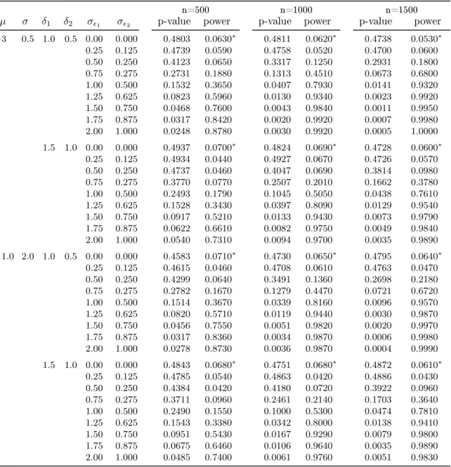
constant. The results are presented in table 4 and for one parameter constellation in gure 1. As can be seen the asymptotic power is aected by the number of observations and the variation ofδt. Theαerror lies between5%and 7%. We see, that the signicance level is

achieved even in small samples (n=500). The test power increases with more observations and higher variation in the dynamic model. For small sample size (n=500) the selectivity of the test is only acceptable for σ1 = 2 and σ2 = 1 with a β error of 13% to 26%. For

n = 1000 instead, the asymptotic distribution of the test seems to hold, even when the

σs are smaller. When variations are small, e.g. σ1 = 0.25 and σ2 = 0.125then the test

doesn't detect this deviation from constancy of the copula parameter. We conclude, that the test holds the signicance level and has reasonable power at least when sample size is large (n=1000) and the variation is not too small (σ1 ≈1.25and σ2 ≈0.5).

5 Empirical analysis

In this section we investigate the potential of the dynamic copula-based Markov model for nancial data compared to a usual GARCH(1,1) model.

5.1 Preliminary analysis

We chose daily log returns of Commerzbank from 18th April 2001 to 31th March 2010. To get an overview of the data we did some descriptive statistics and the KPSS test on stationarity and Jarque-Bera test for normality. As can be seen in table 1 the observations are skewed, leptokurtic, stationary and not normally distributed.

Table 1: Descriptive statistics of Commerzbank daily log returns

n mean std.dev. skewness kurtosis p-value of KPSS p-value of JB

Since we are modeling dependence structures we computed some common dependence measures: the linear correlation ρ, Spearman's Rho ρS and Kendall's Tau τ. Following

[Cont, 2001] we use ρ[α] = ρ[|Xt−1|α,|Xt|α] as a measure of nonlinear dependence. For α = 2volatility clustering, already mentioned in the introduction, can be measured. The

results are presented in table 2.

Table 2: Intertemporal dependence in Commerzbank daily log returns

ρ ρS τ ρ[1] ρ[2]

0.0791 0.0216 0.0134 0.3936 0.2475

The log returns show a slight slight positive correlation regarding rho ρS and τ. The

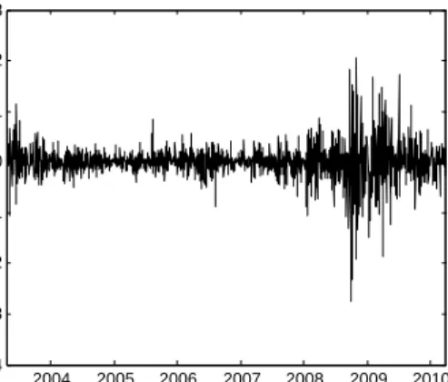
nonlinear measures show a higher amount and especially forα= 2we can assume volatility

clustering. This is not surprising because gure 2 pictures this phenomenon. Because GARCH models take the volatility clustering into account, our approach to compare the copula-based Markov model with a GARCH(1,1) model is supported.

5.2 Parameter estimation

We assumed the IFM method, thus the parameters are estimated in two steps. First, we t the marginal distribution and follow two approaches:

Parametric and empirical distribution We t a hyperbolic distribution f(x) = ψ 2_−η2 2ψσK1(σ p ψ2_−η2₎exp −ψpσ2_{+ (x−µ)}2_+η(x−µ)

with ψ >0 , 0 ≤ |η|< ψ , µ∈ _R ,σ ≥0 and K1 is the modied bessel function of 2nd

order. As benchmark we use the gaussian distribution. The reason for choosing the hyper-bolic distribution is due its ability in modeling skewness as well as heavy tails, which is a well-known so-called stylized fact of nancial returns. The hyperbolic distribution has been investigated in nancial market models as by [Jaschke, 2000],[Eberlein & Keller, 1995] or [Reimann, 2005] among others. Moreover, [Eberlein & Keller, 1995] found evidence for stock returns to follow a hyperbolic distribution. In addition to the full parametric ap-proach, a semi-parametric is chosen, where the marginal distributions are estimated using the empirical distribution Fn(x) = 1_nPnt=11(−∞,x](Xt) can be applied. This encompasses

the approach of [Genest et al., 1995]. GARCH

and [Bollerslev, 1986] suggested ARCH resp. GARCH models to capture this phenom-ena. Therefore, we adapt a standard GARCH(1,1) with gaussian innovations to the data and compare its performance with the copula-based Markov approach. Note that a GARCH(1,1) is clearly not Markovian, but a martingale dierence. So we compare en passant two dierent types of stochastic processes, namely Markov chains and martingale dierences.

The GARCH(1,1) process can be dened by xt|Ft−1 ∼ N(0, σ2t) with σt2 = ω+αx2t−1+ βσ_t2₋₁ and ω >0, α, β ≥0.

The residuals ut=σt−1xt withut∼ N(0,1)are then GARCH-ltered log returns.

We proceed with the estimation of the copula parameters. For the hyperbolic margins and the margins estimated with the empirical distribution function the score test for dy-namic copula parameters is performed. For the GARCH ltered innovations we also t our copula-based Markov model and we test whether there is still some dynamics in the dependence structure. If this were the case, we would have evidence that there is time-variation not only in the conditional variances but also in other moments. If instead the null cannot be rejected, we can conclude that all sort of time variation is already captured by the GARCH(1,1)-model. The only way a copula may now help in modeling the ltered GARCH(1,1)-residuals is just due to the fact, that we have assumed gaussian innovations, which is usually not convenient. Instead other distributions like skewed t-distributions as proposed in [Hansen, 1994] or [Chen, 2007] would be preferable. But the focus lies not on modeling the conditional distribution as exact as possible, but to elaborate the benet of dynamic copula-based Markov models over the standard GARCH(1,1) models.

If the null hypothesis of constant copula parameters is rejected, we model a dynamic copula parameter. For the score-test we assumed the variation in 6. The aim was to expose any kind of variation. In a next step we modelδtas a modied ARMA(1,k) process, as proposed

in [Abegaz & Naik-Nimbalkar, 2008]:

δt= exp ω+αlog(δt−1) +β 1 k k X i=1 |ut−1−ut−i−1| ! .

This approach includes an autoregressive termδt−1and an error term for the mean absolute

dierence betweenutandut−1, which captures variation in the dependence structure. The uts are estimated byuˆt=F(xt;θˆ). δ1 is assumed to be constant.

5.3 Results

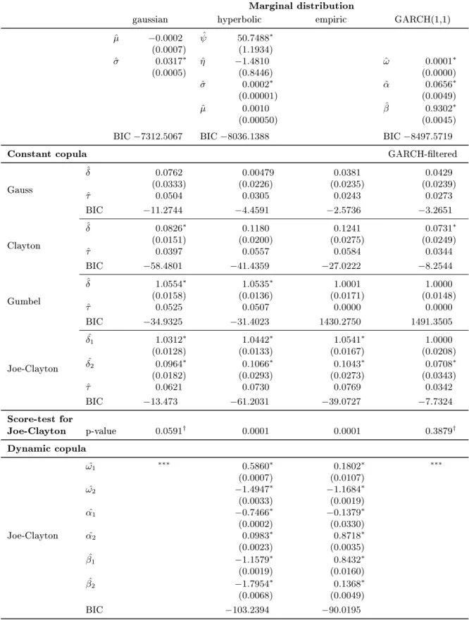
The results for Commerzbank daily stock returns are summarized in table 5. Regarding to the Bayesian Information Criterion (BIC) for the marginal distributions it can be seen that the hyperbolic distribution performs better than the gaussian one. The GARCH(1,1)

model achieves the best t due to BIC.

For the GARCH residuals we did some further investigation and tested them for autocorre-lation with a Ljung-Box test and for normality with a Jarque-Bera test (see table 3). If we had signicance against the Null of no serial correlation, we would still have some relevant information in our model, and thus we just re-identify our GARCH-model, by taking higher orders or an AR(p)-process for the conditional mean. But this would contradict economic theory, where the ecient market and the rational expectations hypothesis of the nancial actors contains that the conditional return of an asset should be zero, i.e. E[Rt|Ft−1] = 0,

because otherwise there is a systematic information about the behavior of the stock return and everyone will buy (if we had positive trend) or sell the asset. The null hypothesis of no correlation can be rejected for assuming dierent lags. As our times series includes 2363 observations we report the results of the Ljung-Box test of order 20 in table 3. Also the residuals are not normal distributed, the main focuss lies on the non-presence of auto-correlation in the residuals, the absolute values of the residuals and the squared residuals. Thus we can assume that the ltered residuals are not following a gaussian white noise process, but they are white noise and that the conditional distribution of the GARCH(1,1) model is misspeced. The t could have been improved by assuming student-t distributed residuals or a higher order GARCH process. To simplify matters we will not follow this.

Table 3: Tests of the GARCH residuals

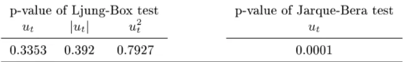
p-value of Ljung-Box test p-value of Jarque-Bera test

ut |ut| u2t ut

0.3353 0.392 0.7927 0.0001

Next, we estimated the parameters of the copulas, proposed in section 2.1. For the gaus-sian and the ltered GARCH innovations the clayton and for the hyperbolic and empirical distribution the Joe-Clayton copula performs best, regarding BIC. So our generalization of the score-test to two-parametric copulas seems to be helpful. The Gumbel copula per-forms worst and is inappropriate for our data set. We also computed Kendall's Tau from the estimated copula parametersδ. Next we applied the generalized score-test for the

Joe-Clayton copula and the Joe-Clayton copula. The null hypothesis of constant copula parameters is rejected for all marginal distributions except the gaussian and the ltered GARCH in-novations. Modeling dynamic copulas improves the t in both other cases. To sum up we compare the dynamic Joe-Clayton copula with hyperbolic margins and 10 parameters, with an added up BIC of−8,139.4, to a simple GARCH(1,1) model with three parameters and

a BIC of−8,497.6. It gets clear that there is no advantage of the (dynamic) copula-based

Markov chain model for the log returns. Our approach to improve the usual GARCH(1,1) model by applying the copula-based Markov model on the residuals, brings few improve-ment of the t. Note that the choice of the Clayton copula corresponds to the stylized fact,

that (extreme) negative returns are more likely then positives. As the Clayton copula cov-ers negative tail dependence, it can be concluded that the ltered GARCH residuals still exhibits signicant lower tail dependence which encompasses the aforementioned stylized fact. Note that this phenomena could have been captured by taking a skewed conditional distribution in our GARCH model.

6 Conclusion

In our paper we gave a short review on dynamic copula-based Markov models and general-ized the score-test proposed by [Abegaz & Naik-Nimbalkar, 2008]. The null hypothesis of no time variation in the parameters of our copula models is extended to variation in at least one of the possible multidimensional parameter sets. The signicance level is maintained when a Joe-Clayton copula, which has two parameters, is investigated. The test power increases with more observations, but it is general lower than in one-dimensional parameter case. This result is not astonishing as we would reject the null, when there is time varia-tion in at least one parameter. To show that the generalizavaria-tion is useful, we modeled the daily returns of the Commerzbank stock using dierent copulas. We found evidence that the very exible Joe-Clayton copula outperforms the other one parametric copula models. After estimating the margins with hyperbolic distribution as well as the gaussian and the empirical distribution, the possible dynamics in the parameter is investigated. We see that the null is rejected for all copulas except for the gaussian and the. In a next step we set up as a benchmark model a standard GARCH(1,1) model with gaussian innovations. An-alyzing the residuals, we found no evidence against white noise, but the distribution still exhibits skewness. This may be captured by adapting a more realistic distribution like a skewed-t or hyperbolic. The main advantage of the standard GARCH(1,1) lies in the fact that it is numerical preferable as it is fast and quite easy to estimate, has less parame-ters compared with dynamic copula-based Markov models. Moreover, it is able to capture volatility clusters and its easy applicability to VaR calculations, portfolio optimization and option-pricing. Therefore, the question may arise, whether Markov chains are suitable models for stock returns at all or that martingale dierence equation like GARCH(1,1) are more able to capture stylized facts that stock returns exhibit.

Mathematical appendix

A: Assumptions

Following [Abegaz & Naik-Nimbalkar, 2008] and [White, 1994], resp. [Patton, 2002] p.112 . we post the following assumptions:

A1. The process (Xt)t∈N is stationary andα-mixing, with mixing coecient α(n), such

thatP∞

n=1α(n)

β

2(2+β) _<∞, for _{β >0}.

A2. (ˆθ,δˆ) is the two-stage maximum likelihood estimator and thus solution of the

maxi-mization problem (4) resp. (5).

A3. (a) f(xt|xt−1; Θ)>0P-a.s. independent ofΘ, and twice continuously dierentiable

on Ω.

(b) The copula densities are twice continuously dierentiable onΩd2_.

(c) There exists neighborhoodsUθ and Uδ such that we have for all θ∈Uθ ⊂Ωd1

and δ∈UδΩd2: i. E sup θ |∇_θf(xt;θ)| <∞,E sup δ |∇_δc(ut, ut−1;δ)| <∞ ii. E sup θ |∇θθf(xt;θ)| <∞,E sup δ |∇δδc(ut, ut−1;δ)| <∞ iii. E sup θ |∇_θθlogf(xt;θ)| <∞,E sup δ |∇_δδlogc(ut, ut−1;δ)| <∞

A4. For all θ ∈ Uθ ⊂ Ωd1 and δ ∈ Uδ ⊂ Ωd2 we have, that −E[∇θθlogf(xt;θ)], V ar(∇θlogf(xt;θ)), −E[∇δδlogc(ut, ut−1;δ)], V ar(∇δlogc(ut, ut−1;δ)) are O(1)

and uniformly positive denite.

A5. E[|Wt,j(θ,δ)|2+β]<∞for β >0,j = 1,2 and allt≥1 and

lim n→∞ 1 n n X t=1 E[W_t,j2 (θ,δ)|Ft−1] =σ2j >0, a.s.

Note the minor modication compared to [Abegaz & Naik-Nimbalkar, 2008], especially the assumptions in A3 that are needed to ensure consistency of the the two-stage maximum-likelihood estimator are less strong than in for instance [Joe, 1997] p.318. To obtain locally asymptotic normally distributed estimators the twice continuously dierentiability assump-tion on the densities is sucient, see [Ferguson, 1996] p.119 . The uniformly integrability for the score functions and the densities are needed, on the one hand side to make use of the weak law of large numbers forα- mixing processes, see for instance [White, 1984], and

to interchange dierentiation and integration, see [Ferguson, 1996] p.124.

B: Proofs

Proof of lemma 1 First note that S(θ,δ) is a martingale under A1 and A3 and that

S(θ,δ) = 1₂Pn

martingales in [Basawa & Rao, 1980] p.388 to conclude, that n−1/2 n X t=2 Wt(θ,δ) d →N(0,σ2),

whereσ2=E[Wt(θ,δ)Wt(θ,δ)0]. Finally we have:

S(θ,δ) = 1 2 n X t=2 Wt(θ,δ) d →N(0,1/4σ2).

Proof of lemma 2 Denote the maximum likelihood estimator by _θˆ _{obtained in a rst}

step by maximizing (4) as the solution of the corresponding score equation Sθ(θ) = 0.

Then we have under the conditions A3, that 1 nSθ(ˆθ)

a.s.

→ E[Sθ(ˆθ)] = 0d1×1, where 0d1×1

is a vector of zeros with length d1. Making a rst order Taylor series expansion of S(ˆθ)

around the true parameter vectorS(θ0) we get:

Sθ(ˆθ) = Sθ(θ0) +∇θSθ(θ0)(ˆθ−θ0) +oP(1) 1 nSθ(ˆθ) ∼ = 1 nSθ(θ0) + 1 n∇θSθ(θ0)(ˆθ−θ0)

Rearranging leads to:

n1/2(ˆθ−θ0) = −1 n∇θSθ(θ0) −1 n−1/2Sθ(θ0).

For the rst equation we have

−1 n∇θSθ(θ0) −1 a.s. → E[∇_θSθ(θ0)]−1 =D−1,

which is just the inverse of hessian of the the log-likelihood problem (4). Due to assumption A4 the matrix D is invertible at least in Uθ. The second term n−1/2Sθ(θ0) is just a

continuous function of anα-mixing process and thus is itselfα-mixing, see [Davidson, 1994]

theorem 14.1. For completeness we present a result due to [Denker, 1986]:

Theorem 4 Let (Xn)n∈N be strictly stationary α-mixing sequence, i.e. E[X1] = 0 and E[|X1|2+δ]<∞with mixing coecient α(n), s.t.

P∞ n=1α(n) δ 2(2+δ) _<∞and_lim n→∞σn2 = ∞. Set Sn=Pni=1Xi, then n1/2Sn/σn→d N(0, σ2), where σ2 = E[X₁2] + 2P∞

n=1E[X1X1+n], i the sequence {S2n/σ2n, n ≥ 1} is uniformly

Under the assumptions imposed on the process (Xt)t∈Nwe have that Sθ(θ0) = n X t=1 ∇θlogf(xt;θ0)

fullls the the assumptions of theorem 4, withE[X₁2] =E[∇θlogf(x1;θ0)∇0_θlogf(x1;θ0)]

and P∞

n=1E[X1X1+n] =

P∞

k=1E[∇θlogf(x1;θ0)∇0θlogf(x1+k;θ0)]. Summarizing we

have n−1/2Sθ(θ0)→d N(0, V), where V =E[∇θlogf(x1;θ0)∇0θlogf(x1;θ0)] + 2 ∞ X k=1 E[∇θlogf(x1;θ0)∇0θlogf(x1+k;θ0)].

We nally get the result of lemma 2 by applying Slutzky's theorem.

Proof of lemma 3 Lemma 3 can be proven in exactly the same way as lemma 2 or seen as a direct consequence of theorem 6.11 in [White, 1994], therefore, it is omitted here. For a detailed proof see [Reichert, 2010] p.46 . If the model is correctly specied, the result for the asymptotic variance of the two-stage estimator simplies to the form given in lemma 3. Also note that our parameter-vector Θ = (θ,δ) is separable in the sense, that there is

no dependency betweenθ and δ, therefore, E[SθSδ] = 0.

Proof of lemma 4 First we have for i= 1, ..., d1 and j= 1...d2:

1 n ∂S(θ,δ)j ∂θi = 1 n         n X t=2 ∂2 ∂θi∂21,j log  c(ut−1, ut;δ) + 1 2 d2 X j=1 ∂2c(ut−1, ut;δ) ∂δ2 j σ1,j   | {z } :=Nt(ut−1, ut;δ)         σ2 1=0 . We have E " −∂ 2_N t(ut−1, ut;δ) ∂δi∂σ21,j # σ2 ₁=0 =E " ∂Nt(ut−1, ut;δ) ∂θi ∂Nt(ut−1, ut;δ) ∂σ2 1,j # σ2 ₁=0 .

Some calculation yields:

∂Nt(ut−1, ut;δ) ∂σ2 1,j = 1 2Wt,j(θ,δ) ∂Nt(ut−1, ut;δ) ∂θi = ∇_θilogct(θ).

Using the ergodic theorem we can nally conclude that: lim n→∞ 1 n ∂S(θ,δ)j ∂θi = E " ∂Nt(ut−1, ut;δ) ∂θi ∂Nt(ut−1, ut;δ) ∂σ2 1,j # σ2 ₁=0 = E −1 2Wt,j(θ,δ)∇ 0 θilogct(θ) σ2 1=0 := σθ,ij And thus lim n→∞ 1 n ∂S(θ,δ) ∂θ =σθ,

whereσθ is just as in theorem 3.

The second assertion of lemma 4 can be proven in exactly the same manner.

Proof of theorem 3 We have forn→ ∞:

n−1/2S(ˆθ,δˆ) =n−1/2S(θ0,δ0) + 1 n∇θS(θ0,δ0)n 1/2_(ˆθ−θ 0) + 1 n∇δS(θ0,δ0)n 1/2_(ˆδ−δ 0).

With the results from lemma 2-4 we have:

= n−1/2S(θ0,δ0)−σθD−1n−1/2Sθ(θ0)−σδI−δδ1n

−1/2_S

δ(θ0,δ0)−σδI−δδ1IδθD−1n−1/2Sθ(θ0)

= n−1/2S(θ0,δ0)−σδI−_δδ1n−1/2Sδ(θ0,δ0)−(σθ+σδI−_δδ1Iδθ)D−1n−1/2Sθ(θ0).

Now we have to calculate the covariances betweenS(θ0,δ0),Sθ(θ) and Sδ(θ0,δ0). First,

as there is no dependency between δandθ we haveCov(Sθ,Sδ) = 0. Moreover, we have: Cov[S(θ0,δ0),Sθ(θ0)] = E[S(θ0,δ0)Sθ(θ0)0]−E[S(θ0,δ0)]E[Sθ0(θ0) 0_] = n X t=2 E 1 2Wt(θ0,δ0)∇θlogf(xt;θ0) 0 − n X t=2 E 1 2Wt(θ0,δ0) n X t=2 E∇θlogf(xt;θ0)0 = 0.

Note that E[Wt(θ0,δ0)∇0θlogf(xt;θ)] = 0, because for every combination of {r, s, t ∈ 0,1, ...}of E[Wr,s(θ0,δ0)∇0_θlogf(xt;θ)] = 0we have: R R R R R R 1 c(F(xr;θ),F(xs;θ);δ) ∂2_c(F(x r;θ),F(xs;θ);δ) ∂δ2 ∂logf(xt,θ) ∂θ f(xr, xs, xt;θ,δ)dxrdxsdxt =R R R R R R 1 c(F(xr;θ),F(xs;θ);δ) ∂2_c(F(x r;θ),F(xs;θ);δ) ∂δ2 1 f(xt;θ) ∂f(xt;θ) ∂θ ×f(xr;θ)f(xs;θ)f(xt;θ)c(F(xr;θ), F(xs;θ);δ)c(F(xs;θ), F(xt;θ);δ)dxrdxsdxt =R R R R R R ∂2_c(F(x r;θ),F(xs;θ);δ) ∂δ2 ∂f(xt,θ) ∂θ f(xr;θ)f(xs;θ)c(F(xs;θ), F(xt;θ);δ)dxrdxsdxt =R_RR_RR_R∂f(xt;θ) ∂θ c(F(xs;θ), F(xt;θ);δ)f(xs;θ) n ∂2c(F(xr;θ),F(xs;θ);δ)f(xr;θ) ∂δ2 o dxrdxsdxt =R R R R ∂f(xt;θ) ∂θ c(F(xs;θ), F(xt;θ);δ)f(xs;θ) n R R ∂2_c(F(x r;θ),F(xs;θ);δ)f(xr;θ) ∂δ2 dxr o dxsdxt =R R R R ∂f(xt;θ) ∂θ c(F(xs;θ), F(xt;θ);δ)f(xs;θ) n ∂2 ∂δ2 R Rf(xr|xs;θ,δ)dxr o | {z } =0 dxsdxt =0.

Finally we can conclude that

Cov(S(θ,δ),Sδ(θ,δ)) = n X t=2 E 1 2Wt(θ0,δ0)∇ 0 δlogc(ut, ut−1,θ) = (n−1)σδ.

Putting the results together we get:

   n−1/2S(θ0,δ0) n−1/2Sδ(θ0,δ0) n−1/2_S θ(θ0,δ0)    d →N       0 0 0   ,    σ/4 σδ/n 0 σδ/n Iδδ 0 0 0 V      .

Thus we nally get:

n−1/2S(ˆθ,δˆ)→d N(0,Σ),

withΣjust as in theorem 3.

Tables and Figures

Figure 1: Power of the general score-test

2004 2005 2006 2007 2008 2009 2010 −0.4 −0.3 −0.2 −0.1 0 0.1 0.2 0.3 Zeit Rendite Commerzbank

Table 4: Power of the score-test with Joe-Clayton copula and normal margins

n=500 n=1000 n=1500

µ σ δ1 δ2 σ1 σ2 p-value power p-value power p-value power

−3 0.5 1.0 0.5 0.00 0.000 0.4803 0.0630∗ 0.4811 0.0620∗ 0.4738 0.0530∗ 0.25 0.125 0.4739 0.0590 0.4758 0.0520 0.4700 0.0600 0.50 0.250 0.4123 0.0650 0.3317 0.1250 0.2931 0.1800 0.75 0.275 0.2731 0.1880 0.1313 0.4510 0.0673 0.6800 1.00 0.500 0.1532 0.3650 0.0407 0.7930 0.0141 0.9320 1.25 0.625 0.0823 0.5960 0.0130 0.9340 0.0023 0.9920 1.50 0.750 0.0468 0.7600 0.0043 0.9840 0.0011 0.9950 1.75 0.875 0.0317 0.8420 0.0020 0.9920 0.0007 0.9980 2.00 1.000 0.0248 0.8780 0.0030 0.9920 0.0005 1.0000 1.5 1.0 0.00 0.000 0.4937 0.0700∗ 0.4824 0.0690∗ 0.4728 0.0600∗ 0.25 0.125 0.4934 0.0440 0.4927 0.0670 0.4726 0.0570 0.50 0.250 0.4737 0.0460 0.4047 0.0690 0.3814 0.0980 0.75 0.275 0.3770 0.0770 0.2507 0.2010 0.1662 0.3780 1.00 0.500 0.2493 0.1790 0.1045 0.5050 0.0438 0.7610 1.25 0.625 0.1528 0.3430 0.0397 0.8090 0.0129 0.9540 1.50 0.750 0.0917 0.5210 0.0133 0.9430 0.0073 0.9790 1.75 0.875 0.0622 0.6610 0.0082 0.9750 0.0049 0.9840 2.00 1.000 0.0540 0.7310 0.0094 0.9700 0.0035 0.9890 1.0 2.0 1.0 0.5 0.00 0.000 0.4583 0.0710∗ 0.4730 0.0650∗ 0.4795 0.0640∗ 0.25 0.125 0.4615 0.0460 0.4708 0.0610 0.4763 0.0470 0.50 0.250 0.4299 0.0640 0.3491 0.1360 0.2698 0.2180 0.75 0.275 0.2782 0.1670 0.1279 0.4470 0.0721 0.6720 1.00 0.500 0.1514 0.3670 0.0339 0.8160 0.0096 0.9570 1.25 0.625 0.0820 0.5710 0.0119 0.9440 0.0030 0.9870 1.50 0.750 0.0456 0.7550 0.0051 0.9820 0.0020 0.9970 1.75 0.875 0.0317 0.8360 0.0034 0.9870 0.0006 0.9980 2.00 1.000 0.0278 0.8730 0.0036 0.9870 0.0004 0.9990 1.5 1.0 0.00 0.000 0.4843 0.0680∗ 0.4751 0.0680∗ 0.4872 0.0610∗ 0.25 0.125 0.4785 0.0540 0.4863 0.0420 0.4886 0.0430 0.50 0.250 0.4384 0.0420 0.4180 0.0720 0.3922 0.0960 0.75 0.275 0.3711 0.0960 0.2461 0.2140 0.1703 0.3640 1.00 0.500 0.2490 0.1550 0.1000 0.5300 0.0474 0.7810 1.25 0.625 0.1543 0.3380 0.0342 0.8000 0.0138 0.9410 1.50 0.750 0.0951 0.5430 0.0167 0.9290 0.0079 0.9800 1.75 0.875 0.0675 0.6460 0.0106 0.9640 0.0035 0.9890 2.00 1.000 0.0485 0.7400 0.0061 0.9760 0.0051 0.9830

REMARK: The means of 1000 replications of the p-values of the genaral score-test and the power are displayed for dierent parameter constellations. Theαerrors are marked with∗and describe how often the null hypothesis is

Table 5: Estimates for the daily log returns of Commerzbank

Marginal distribution

gaussian hyperbolic empiric GARCH(1,1)

ˆ µ −0.0002 ψˆ 50.7488∗ (0.0007) (1.1934) ˆ σ 0.0317∗ ηˆ −1.4810 ωˆ 0.0001∗ (0.0005) (0.8446) (0.0000) ˆ σ 0.0002∗ αˆ 0.0656∗ (0.00001) (0.0049) ˆ µ 0.0010 βˆ 0.9302∗ (0.00050) (0.0045)

BIC−7312.5067 BIC−8036.1388 BIC−8497.5719

Constant copula GARCH-ltered

Gauss ˆ δ 0.0762 0.00479 0.0381 0.0429 (0.0333) (0.0226) (0.0235) (0.0239) ˆ τ 0.0504 0.0305 0.0243 0.0273 BIC −11.2744 −4.4591 −2.5736 −3.2651 Clayton ˆ δ 0.0826∗ 0.1180 0.1241 0.0731∗ (0.0151) (0.0200) (0.0275) (0.0249) ˆ τ 0.0397 0.0557 0.0584 0.0344 BIC −58.4801 −41.4359 −27.0222 −8.2544 Gumbel ˆ δ 1.0554∗ 1.0535∗ 1.0001 1.0000 (0.0158) (0.0136) (0.0171) (0.0148) ˆ τ 0.0525 0.0507 0.0000 0.0000 BIC −34.9325 −31.4023 1430.2750 1491.3505 Joe-Clayton ˆ δ1 1.0312∗ 1.0442∗ 1.0541∗ 1.0000 (0.0128) (0.0133) (0.0167) (0.0208) ˆ δ2 0.0964∗ 0.1066∗ 0.1043∗ 0.0708∗ (0.0182) (0.0293) (0.0273) (0.0343) ˆ τ 0.0621 0.0730 0.0769 0.0342 BIC −13.473 −61.2031 −39.0727 −7.7324 Score-test for Joe-Clayton p-value 0.0591† 0.0001 0.0001 0.3879† Dynamic copula Joe-Clayton ˆ ω1 ∗∗∗ 0.5860∗ 0.1802∗ ∗∗∗ (0.0007) (0.0107) ˆ ω2 −1.4947∗ −1.1684∗ (0.0033) (0.0019) ˆ α1 −0.7466∗ −0.1379∗ (0.0002) (0.0330) ˆ α2 0.0983∗ 0.8718∗ (0.0023) (0.0035) ˆ β1 −1.1579∗ 0.8432∗ (0.0019) (0.0160) ˆ β2 −1.7954∗ 0.1368∗ (0.0068) (0.0049) BIC −103.2394 −90.0195

REMARK: Standard errors are embraced. The parameter estimates marked with∗_{are signicant at 5%-level. The}

References

[Abegaz & Naik-Nimbalkar, 2008] Abegaz, F. & Naik-Nimbalkar, U. (2008). Dynamic copula-based markow time series. Communications in Statistics - Theory and Meth-ods, 37, 24472460.

[Basawa & Rao, 1980] Basawa, I. & Rao, B. (1980). Statistical inference for stochastic processes. London: Academic Press.

[Bollerslev, 1986] Bollerslev, T. (1986). Generalized autoregressive conditional het-eroskedasticity. Journal of Econometrics, 31, 307327.

[Chen, 2007] Chen, Y.-T. (2007). Moment-based copula tests for nancial returns. Journal of Business and Economic Statistics, 24, 377397.

[Cont, 2001] Cont, R. (2001). Empirical properties of asset returns: Stylized facts and statistical issues. Quantitative Finance, 1, 223236.

[Davidson, 1994] Davidson, J. (1994). Stochastic limit theory: An introduction for econo-metricians. Oxford: Oxford University Press.

[Denker, 1986] Denker, M. (1986). Uniform integrability and the central limit theorem for strongly mixing processes. In Dependence in probability and statistics, volume 11 (pp. 269289). Boston: Birkhäuser Boston.

[Eberlein & Keller, 1995] Eberlein, E. & Keller, U. (1995). Hyperbolic distributions in nance. Bernoulli, 1, 281299.

[Embrechts et al., 2002] Embrechts, P., McNeil, A., & Strautmann, D. (2002). Correlation and dependence properties in risk management: Properties and pitfalls. Risk Manage-ment: Value-at-risk and beyond. Cambridge: Cambridge University Press.

[Engle, 1982] Engle, R. (1982). Autoregressive conditional heteroscedasticity with esti-mates of variance of united kingdom ination. Econometrica, 50, 9871008.

[Ferguson, 1996] Ferguson, T. (1996). A course in large sample theory. London: Chapman & Hall.

[Genest et al., 1995] Genest, C., Ghoudi, K., & Rivest, L.-P. (1995). A semiparametric estimation procedure of dependence parameters in multivariate families of distributions. Biometrika, 82, 543552.

[Hansen, 1994] Hansen, B. (1994). Autoregressive conditional density estimation. Inter-national Economic Review, 35, 705730.

[Härdle & Okhrin, 2010] Härdle, W. & Okhrin, O. (2010). De copulis non est disputan-dum. Advances in Statistical Analysis, 94, 132.

[Jaschke, 2000] Jaschke, S. (2000). A note on stochastic volatility, GARCH models, and hyperbolic distributions. Working Paper.

[Joe, 1997] Joe, H. (1997). Multivariate models and dependence concepts. New York: Chapman & Hall.

[McNeil et al., 2005] McNeil, A., Frey, R., & Embrechts, P. (2005). Quantitative risk management. Princton: Princton University Press.

[Nelsen, 2006] Nelsen, R. (2006). An introduction to copula. New York: Springer.

[Patton, 2002] Patton, A. (2002). Applications of copula theory in nancial econometrics. PhD thesis, University of California, San Diego.

[Patton, 2006] Patton, A. (2006). Modelling asymmetric exchange rate dependence. In-ternational Economic Review, 47, 527556.

[Rao, 1973] Rao, C. (1973). Linear statistical inference and its application. New York: John Wiley & Sons.

[Reichert, 2010] Reichert, K. (2010). Copulabasierte Modellierung intertemporärer Ab-hängigkeiten. Diploma thesis, Departement of Mathematics, Erlangen.

[Reimann, 2005] Reimann, S. (2005). Evidence for a hyperbolic-like distribution of asset returns drawn from a simple economical nancial markets model. FINRISK Working paper, 212.

[White, 1984] White, H. (1984). Maximum likelihood estimation of misspecied dynamic models. In T. Dijkstra (Ed.), Misspecication analysis. New York: Springer.

[White, 1994] White, H. (1994). Estimation, inference and specication analysis. New York: Cambridge University Press.

[White, 2001] White, H. (2001). Asymptotic theory for econometricians. San Diego: Aca-demic Press.

_____________________________________________________________________

Friedrich-Alexander-Universität

Diskussionspapiere 2011

Discussion Papers 2011

01/2011

Klein, Ingo, Fischer, Matthias, Pleier, Thomas: Weighted Power Mean

Copulas: Theory and Application

02/2011

Kiss, David: The Impact of Peer Ability and Heterogeneity on Student

Achievement: Evidence from a Natural Experiment

03/2011

Zibrowius, Michael: Convergence or divergence? Immigrant wage

assi-milation patterns in Germany

04/2011

Klein, Ingo, Christa, Florian: Families of Copulas closed under the

Con-struction of Generalized Linear Means

05/2011

Schnitzlein, Daniel: How important is the family? Evidence from sibling

correlations in permanent earnings in the US, Germany and Denmark

06/2011

Schnitzlein, Daniel: How important is cultural background for the level

of intergenerational mobility?

07/2011

Steffen Mueller: Teacher Experience and the Class Size Effect -

Experi-mental Evidence

08/2011

Klein, Ingo: Van Zwet Ordering for Fechner Asymmetry

Diskussionspapiere 2010

Discussion Papers 2010

01/2010

Mosthaf, Alexander, Schnabel, Claus and Stephani, Jens: Low-wage

ca-reers: Are there dead-end firms and dead-end jobs?

02/2010

Schlüter, Stephan and Matt Davison: Pricing an European Gas Storage

Facility using a Continuous-Time Spot Price Model with GARCH

Diffu-sion

03/2010

Fischer, Matthias, Gao, Yang and Herrmann, Klaus:

Volatility Models

with Innovations from New Maximum Entropy Densities at Work

04/2010

Schlüter, Stephan, Deuschle, Carola: Using Wavelets for Time Series

Forecasting – Does it Pay Off?

05/2010

Feicht, Robert, Stummer, Wolfgang: Complete closed-form solution to

a stochastic growth model and corresponding speed of economic

re-covery.

_____________________________________________________________________

Friedrich-Alexander-Universität

06/2010

Hirsch, Boris, Schnabel, Claus: Women Move Differently: Job

Separa-tions and Gender.

07/2010

Gartner, Hermann, Schank, Thorsten, Schnabel, Claus: Wage cyclicality

under different regimes of industrial relations.

08/2010

Tinkl, Fabian: A note on Hadamard differentiability and differentiability

in quadratic mean.

09/2010

Tinkl, Fabian: Asymptotic theory for M estimators for martingale

differ-ences with applications to GARCH models.

Diskussionspapiere 2009

Discussion Papers 2009

01/2009

Addison, John T. and Claus Schnabel: Worker Directors: A German

Product that Didn’t Export?

02/2009

Uhde, André and Ulrich Heimeshoff: Consolidation in banking and

fi-nancial stability in Europe: Empirical evidence

03/2009

Gu, Yiquan and Tobias Wenzel: Product Variety, Price Elasticity of

De-mand and Fixed Cost in Spatial Models

04/2009

Schlüter, Stephan: A Two-Factor Model for Electricity Prices with

Dy-namic Volatility

05/2009

Schlüter, Stephan and Fischer, Matthias: A Tail Quantile Approximation

Formula for the Student t and the Symmetric Generalized Hyperbolic

Distribution

06/2009

Ardelean, Vlad: The impacts of outliers on different estimators for

GARCH processes: an empirical study

07/2009

Herrmann, Klaus: Non-Extensitivity versus Informative Moments for

Fi-nancial Models - A Unifying Framework and Empirical Results

08/2009

Herr, Annika: Product differentiation and welfare in a mixed duopoly

with regulated prices: The case of a public and a private hospital

09/2009

Dewenter, Ralf, Haucap, Justus and Wenzel, Tobias: Indirect Network

Effects with Two Salop Circles: The Example of the Music Industry

10/2009

Stuehmeier, Torben and Wenzel, Tobias: Getting Beer During

Commer-cials: Adverse Effects of Ad-Avoidance

11/2009

Klein, Ingo, Köck, Christian and Tinkl, Fabian: Spatial-serial dependency

in multivariate GARCH models and dynamic copulas: A simulation study

_____________________________________________________________________

Friedrich-Alexander-Universität

12/2009

Schlüter, Stephan: Constructing a Quasilinear Moving Average Using

the Scaling Function

13/2009

Blien, Uwe, Dauth, Wolfgang, Schank, Thorsten and Schnabel, Claus:

The institutional context of an “empirical law”: The wage curve under

different regimes of collective bargaining

14/2009

Mosthaf, Alexander, Schank, Thorsten and Schnabel, Claus: Low-wage

employment versus unemployment: Which one provides better

pros-pects for women?

Diskussionspapiere 2008

Discussion Papers 2008

01/2008

Grimm, Veronika and Gregor Zoettl: Strategic Capacity Choice under

Uncertainty: The Impact of Market Structure on Investment and

Wel-fare

02/2008

Grimm, Veronika and Gregor Zoettl: Production under Uncertainty: A

Characterization of Welfare Enhancing and Optimal Price Caps

03/2008

Engelmann, Dirk and Veronika Grimm: Mechanisms for Efficient Voting

with Private Information about Preferences

04/2008

Schnabel, Claus and Joachim Wagner: The Aging of the Unions in West

Germany, 1980-2006

05/2008

Wenzel, Tobias: On the Incentives to Form Strategic Coalitions in ATM

Markets

06/2008

Herrmann, Klaus: Models for Time-varying Moments Using Maximum

Entropy Applied to a Generalized Measure of Volatility

07/2008

Klein, Ingo and Michael Grottke: On J.M. Keynes' “The Principal

Aver-ages and the Laws of Error which Lead to Them” - Refinement and

Ge-neralisation