VR-SGD: A Simple Stochastic Variance Reduction Method for Machine Learning

© 201

8

IEEE. Personal use of this material is permitted. Permission from IEEE must be obtained

for all other uses, in any current or future media, including reprinting/republishing this material

for advertising or promotional purposes, creating new collective works, for resale or

redistribution to servers or lists, or reuse of any copyrighted component of this work in other

works.

VR-SGD: A Simple Stochastic Variance

Reduction Method for Machine Learning

Fanhua Shang,

Member, IEEE,

Kaiwen Zhou, Hongying Liu, James Cheng, Ivor W. Tsang,

Lijun Zhang,

Member, IEEE,

Dacheng Tao,

Fellow, IEEE,

and Licheng Jiao,

Fellow, IEEE

Abstract—In this paper, we propose a simple variant of the original SVRG, called variance reduced stochastic gradient descent (VR-SGD). Unlike the choices of snapshot and starting points in SVRG and its proximal variant, Prox-SVRG, the two vectors of VR-SGD are set to the average and last iterate of the previous epoch, respectively. The settings allow us to use much larger learning rates, and also make our convergence analysis more challenging. We also design two different update rules for smooth and

non-smooth objective functions, respectively, which means that VR-SGD can tackle non-smooth and/or non-strongly convex problems directly without any reduction techniques. Moreover, we analyze the convergence properties of VR-SGD for strongly convex problems, which show that VR-SGD attains linear convergence. Different from most algorithms that have no convergence guarantees for non-strongly convex problems, we also provide the convergence guarantees of VR-SGD for this case, and empirically verify that VR-SGD with varying learning rates achieves similar performance to its momentum accelerated variant that has the optimal convergence rate_O(1/T2). Finally, we apply VR-SGD to solve various machine learning problems, such as convex and non-convex empirical risk minimization, and leading eigenvalue computation. Experimental results show that VR-SGD converges significantly faster than SVRG and Prox-SVRG, and usually outperforms state-of-the-art accelerated methods, e.g., Katyusha.

Index Terms—Stochastic optimization, stochastic gradient descent (SGD), variance reduction, empirical risk minimization, strongly convex and non-strongly convex, smooth and non-smooth

F

1

I

I

opti-mization problem: min x_∈Rd F(x) def = 1 n n ∑ i=1 fi(x) +g(x) (1) wheref(x) =1 n ∑n i=1fi(x),fi(x) :Rd→R, i= 1, . . . , n are

the smooth functions, and g(x)is a relatively simple (but

possibly non-differentiable) convex function (referred to as

a regularizer). The formulation (1) arises in many places in

machine learning, signal processing, data science, statistics

and operations research, such as regularized empirical risk

minimization(ERM). For instance, one popular choice of the

component function fi(·)in binary classification problems

is the logistic loss, i.e.,fi(x) = log(1 + exp(−biaTix)), where

{(a1, b1), . . . ,(an, bn)}is a collection of training examples,

• F. Shang, H. Liu (Corresponding author) and L. Jiao are with the Key Laboratory of Intelligent Perception and Image Understanding of Ministry of Education, School of Artificial Intelligence, Xidian University, China. E-mails:{fhshang, hyliu, lchjiao}@xidian.edu.cn.

• K. Zhou and J. Cheng are with the Department of Computer Science and Engineering, The Chinese University of Hong Kong, Hong Kong. E-mails:

{kwzhou, jcheng}@cse.cuhk.edu.hk.

• I.W. Tsang is with the Centre for Artificial Intelligence, Univer-sity of Technology Sydney, Ultimo, NSW 2007, Australia. E-mail: [email protected].

• L. Zhang is with the National Key Laboratory for Novel Software Technol-ogy, Nanjing University, Nanjing 210023, China. E-mail: [email protected].

• D. Tao is with the UBTECH Sydney Artificial Intelligence Centre and the School of Information Technologies in the Faculty of Engineering and Information Technologies, The University of Sydney, Darlington, NSW 2008, Australia. E-mail: [email protected].

Manuscript received December 19, 2017.

and bi∈ {±1}. Some popular choices for the regularizer

include theℓ2-norm regularizer (i.e.,g(x) = (λ/2)∥x∥2), the

ℓ1-norm regularizer (i.e., g(x) = λ∥x∥1), and the

elastic-net regularizer (i.e., g(x) = (λ1/2)∥x∥2+λ2∥x∥1). Some

other applications include deep neural networks [1], [2],

[3], [4], [5], group Lasso [6], sparse learning and coding

[7], [8], [9], [10], phase retrieval [11], matrix completion

[12], [13], conditional random fields [14], generalized

eigen-decomposition and canonical correlation analysis [15], and

eigenvector computation [16], [17] such as principal

com-ponent analysis (PCA) and singular value decomposition (SVD).

1.1 Stochastic Gradient Descent

We are especially interested in developing efficient

algo-rithms to solve Problem (1) involving the sum of a large

number of component functions. The standard and effective

method for solving (1) is the (proximal) gradient descent

(GD) method, including Nesterov’s accelerated gradient

descent (AGD) [18], [19] and accelerated proximal gradient

(APG) [20], [21]. For the smoothproblem (1), GD takes the

following update rule: starting withx0, and for anyk≥0

xk+1=xk−ηk [ 1 n n ∑ i=1 ∇fi(xk) +∇g(xk) ] (2)

where ηk>0 is commonly referred to as the learning rate

in machine learning or step-size in optimization. Wheng(·)

is non-smooth (e.g., the ℓ1-norm regularizer), we typically

introduce the following proximal operator to replace (2),

xk+1=Proxgηk(yk) := arg min

x_∈Rd { 1 2ηk∥ x−yk∥2+g(x) } (3)

whereyk=xk−(ηk/n) ∑n

i=1∇fi(xk).GD has been proven

to achieve linear convergence forstrongly convexproblems,

and both AGD and APG attain the optimal convergence rate

O(1/T2_{)fornon-strongly convexproblems, whereT denotes}

the number of iterations. However, the per-iteration cost of

all the batch (or deterministic) methods isO(nd), which is

expensive for very largen.

Instead of evaluating the full gradient of f(·) at each

iteration, an efficient alternative is the stochastic (or

in-cremental) gradient descent (SGD) method [22]. SGD only

evaluates the gradient of a single component function at

each iteration, and has muchlowerper-iteration cost,O(d).

Thus, SGD has been successfully applied to many

large-scale learning problems [23], [24], [25], especially training

for deep learning models [2], [3], [26], and its update rule is

xk+1=xk−ηk[∇fik(xk) +∇g(xk)] (4)

whereηk∝1/

√

k, and the indexikcan be chosen uniformly

at random from {1,2, . . . , n}. Although the expectation of

the stochastic gradient estimator∇fik(xk)is anunbiased

es-timation for∇f(xk), i.e.,E[∇fik(xk)] =∇f(xk), the variance

of ∇fik(xk) may be large due to the variance of random

sampling [1]. Thus, stochastic gradient estimators are also

called “noisy gradients”, and we need to gradually reduce its step size, which leads to slow convergence. In particular, even under the strongly convex (SC)condition, standard

S-GD attains a slowersub-linearconvergence rateO(1/T)[27].

1.2 Accelerated SGD

Recently, many SGD methods withvariance reduction have

been proposed, such as stochastic average gradient (SAG)

[28], stochastic variance reduced gradient (SVRG) [1],

s-tochastic dual coordinate ascent (SDCA) [29], SAGA [30],

stochastic primal-dual coordinate (SPDC) [31], and their

proximal variants, such as Prox-SAG [32], Prox-SVRG [33]

and Prox-SDCA [34]. These accelerated SGD methods can

use a constant learning rateη instead of diminishing step

sizes for SGD, and fall into the following three categories:

primal methods such as SVRG and SAGA, dual methods

such as SDCA, and primal-dualmethods such as SPDC. In

essence, many of the primal methods use the full gradient

at the snapshotxeor the average gradient to progressively

reduce the variance of stochastic gradient estimators, as

well as the dual and primal-dual methods, which leads to

a revolution in the area of first-order optimization [35]. Thus, they are also known as the hybrid gradient descent method

[36] or semi-stochastic gradient descent method [37]. In

particular, under the strongly convex condition, most of the accelerated SGD methods enjoy a linear convergence rate (also known as a geometric or exponential rate) and

the oracle complexity ofO((n+L/µ) log(1/ϵ))to obtain an

ϵ-suboptimal solution, where each fi(·) is L-smooth, and

F(·)isµ-strongly convex. The complexity bound shows that

they converge faster than accelerated deterministic

method-s, whose oracle complexity isO(n√L/µlog(1/ϵ))[38], [39].

SVRG [1] and its proximal variant, Prox-SVRG [33], are

particularly attractive because of their low storage

require-ment compared with other methods such as SAG, SAGA and SDCA, which require storage of all the gradients of component functions or dual variables. At the beginning of

thes-th epoch in SVRG, the full gradient∇f(xes−1_)is

com-puted at the snapshotexs−1, which is updated periodically.

Definition 1. The stochastic variance reduced gradient estimator is independently introduced in [1], [36] as follows:

e ∇fis k(x s k) =∇fis k(x s k)− ∇fis k(xe s−1_{) +∇f(xe}s−1_), (5)

wheresis the epoch that iterationkbelongs to.

It is not hard to verify that the variance of the SVRG

estimator ∇efis k(x s k) (i.e., E∥∇efis k(x s k)− ∇f(x s k)∥ 2 ) can be

much smaller than that of the SGD estimator ∇fik(x

s k)

(i.e.,E∥∇fik(xsk)−∇f(x

s k)∥

2_{). Theoretically, fornon-strongly}

convex (Non-SC) problems, the variance reduced methods converge slower than the accelerated batch methods such as

FISTA [21], i.e.,O(1/T)vs.O(1/T2_).

More recently, many acceleration techniques were

pro-posed to further speed up the stochastic variance reduced methods mentioned above. These techniques mainly

in-clude the Nesterov’s acceleration techniques in [24], [38],

[39], [40], [41], reducing the number of gradient

calcula-tions in early iteracalcula-tions [35], [42], [43], the projection-free

property of the conditional gradient method (also known

as the Frank-Wolfe algorithm [44]) as in [45], the stochastic

sufficient decrease technique [46], and the momentum

accel-eration tricks in [35], [47], [48]. [39] proposed an accelerating

Catalyst framework and achieved the oracle complexity

of O((n+√nL/µ) log(L/µ) log(1/ϵ)) for strongly convex

problems. [47] and [49] proved that the accelerated methods

can attain the oracle complexity ofO(nlog(1/ϵ) +√nL/ϵ)

for non-strongly convex problems. The overall

complexi-ty matches the theoretical upper bound provided in [50].

Katyusha [47], point-SAGA [51] and MiG [49] achieve the

best-known oracle complexity ofO((n+√nL/µ) log(1/ϵ))

for strongly convex problems, which is identical to the

upper complexity bound in [50]. Hence, Katyusha and MiG

are thebest-knownstochastic optimization method for both

SCandNon-SCproblems, as pointed out in [50]. However, selecting the best values for the parameters in the accel-erated methods (e.g., the momentum parameter) is still an open problem. In particular, most of accelerated stochastic variance reduction methods, including Katyusha, require at least one auxiliary variable and one momentum parameter, which lead to complicated algorithm design and high per-iteration complexity, especially for very high-dimensional and sparse data.

1.3 Our Contributions

From the above discussions, we can see that most of the accelerated stochastic variance reduction methods such

as [35], [38], [43], [45], [46], [47], [52], [53] and applications

such as [7], [9], [10], [13], [16], [17] are based on the SVRG

method [1]. Thus, any key improvement on SVRG is very

important for the research of stochastic optimization. In this

paper, we propose a simple variant of the original SVRG [1],

called variance reduced stochastic gradient descent (VR-SGD).

The snapshot point and starting point of each epoch in

VR-SGD are set to the average and last iterate of the previous

epoch, respectively. This is different from the settings of

SVRG and Prox-SVRG [33], where the two points of the

TABLE 1

Comparison of convergence rates of VR-SGD and its counterparts. SVRG [1] Prox-SVRG [33] VR-SGD SC, smooth linear rate unknown linear rate SC, non-smooth unknown linear rate linear rate Non-SC, smooth unknown unknown O(1/T)

Non-SC, non-smooth unknown unknown O(1/T)

set to be the average of the previous epoch. This difference makes the convergence analysis of VR-SGD significantly more challenging than that of SVRG and Prox-SVRG. Our empirical results show that the performance of VR-SGD is significantly better than its counterparts, SVRG and Prox-SVRG. Impressively, VR-SGD with varying learning rates achieves better or at least comparable performance with

ac-celerated methods, such as Catalyst [39] and Katyusha [47].

The main contributions of this paper are summarized below.

• The snapshot and starting points of VR-SGD are set

to two different vectors, i.e.,xes=_m1∑m_k=1xs_k (Option

I) orxes=_m1₋₁∑_km₌₁−1xs_k(Option II), andxs₀+1=xs_m. In

particular, we find that the settings of VR-SGD allow

us to take much larger learning rates than SVRG,

e.g., 1/L vs. 1/(10L), and thus significantly speed

up its convergence in practice. Moreover, VR-SGD

has an advantage over SVRG in terms ofrobustness

of learning rate selection.

• Unlike proximal stochastic gradient methods, e.g.,

Prox-SVRG and Katyusha, which have a unified

update rule for the two cases of smooth and

non-smooth objectives (see Section 2.2 for details), VR-SGD employs two different update rules for the

two cases, respectively, as in (12) and (13) below.

Empirical results show that gradient update rules as

in (12) for smooth optimization problems are better

choices than proximal update formulas as in (10).

• We provide the convergence guarantees of VR-SGD

for solving smooth/non-smooth and non-strongly

convex(or general convex) functions. In comparison, SVRG and Prox-SVRG do not have any convergence

guarantees, as shown in Table1.

• Moreover, we also present a momentum accelerated

variant of VR-SGD, discuss their equivalent relation-ship, and empirically verify that they achieve similar performance to their variant that attains the optimal

convergence rateO(1/T2₎

.

• Finally, we theoretically analyze the convergence

properties of VR-SGD with Option I or Option II for

smooth/non-smooth and strongly convex functions,

which show that VR-SGD attainslinearconvergence.

2

P

R

W

Throughout this paper, we use∥·∥to denote the ℓ2-norm

(also known as the standard Euclidean norm), and∥·∥1 is

the ℓ1-norm, i.e., ∥x∥1 =∑di=1|xi|. ∇f(·) denotes the full

gradient off(·)if it is differentiable, or∂f(·)the subgradient

iff(·)is only Lipschitz continuous. For each epochs∈[S]

and inner iterationk∈{0,1, . . . , m−1},is_k∈[n]is the random

chosen index. We mostly focus on the case of Problem (1)

Algorithm 1SVRG (Option I) and Prox-SVRG (Option II)

Input: The number of epochsS, the number of iterationsm

per epoch, and the learning rateη.

Initialize: xe0_. 1: fors= 1,2, . . . , Sdo 2: µes= 1_n∑n_i=1∇fi(xes−1), xs0=ex s₋1 ; 3: fork= 0,1, . . . , m−1do 4: Pickis

kuniformly at random from[n];

5: ∇efis k(x s k) =∇fis k(x s k)− ∇fis k(xe s−1_{) +µe}s_; 6: Option I:xs k+1=xsk−η [ e ∇fis k(x s k) +∇g(xsk) ] , orxs k+1=Prox g η ( xs k−η∇efis k(x s k) ) ; 7: Option II: xs_k+1= arg miny∈Rd { g(y)+yT∇efis k(x s k)+ 1 2η∥y−x s k∥ 2} ; 8: end for 9: Option I: xes_=xs

m; //Last iterate for snapshotxe

10: Option II:exs=_m1∑_km₌₁xs_k; //Iterate averaging forxe

11: end for Output: xeS

when eachfi(·)isL-smooth1, andF(·)isµ-strongly convex.

The two common assumptions are defined as follows.

2.1 Basic Assumptions

Assumption 1(Smoothness). Eachfi(·)isL-smooth, that is,

there exists a constantL >0such that for allx, y∈Rd,

∥∇fi(x)− ∇fi(y)∥ ≤L∥x−y∥. (6) Assumption 2(Strong Convexity).F(x)isµ-strongly convex, i.e., there exists a constantµ >0such that for allx, y∈Rd_,

F(y)≥F(x) +⟨∇F(x), y−x⟩+µ

2∥x−y∥

2_.

(7)

Note that wheng(·)is non-smooth, the inequality in (7)

needs to be revised by simply replacing the gradient∇F(x)

with an arbitrary sub-gradient of F(·) at x. In contrast,

for a non-strongly convex or general convex function, the

inequality in (7) can always be satisfied withµ= 0.

2.2 Related Work

To speed up standard and proximal SGD, many stochastic

variance reduced methods [28], [29], [30], [36] have been

proposed for some special cases of Problem (1). In the case

when each fi(x) is L-smooth, f(x) is µ-strongly convex,

andg(x)≡0, Rouxet al.[28] proposed a stochastic average

gradient (SAG) method, which attains linear convergence. However, SAG, as well as other incremental aggregated

gra-dient methods such as SAGA [30], needs to store all

gradi-ents, so thatO(nd)memory is required in general [42].

Sim-ilarly, SDCA [29] requires storage of all dual variables [1],

which usesO(n)memory. In contrast, SVRG proposed by

Johnson and Zhang [1], as well as Prox-SVRG [33], has the

similar convergence rate to SAG and SDCA, but without the memory requirements of all gradients and dual variables.

In particular, the SVRG estimator in (5) may be the most

1. In fact, we can extend the theoretical results for the case, when the gradients of all component functions have the same Lipschitz constant

L, to the more general case, when some component functionsfi(·)have

popular choice forstochastic gradient estimators. The update

rule of SVRG for the case of Problem (1) wheng(·)≡0is

xs_k+1=xs_k−η∇efis k(x

s

k). (8)

When the smooth regularizerg(·)̸= 0, the update rule in

(8) becomes: xs

k+1 =xsk−η[∇efis k(x

s

k) +∇g(xsk)]. Although

the original SVRG in [1] only has convergence guarantees

for the special case of Problem (1), when eachfi(x)is L

-smooth, f(x) is µ-strongly convex, and g(x)≡0, we can

extend SVRG to the proximal setting by introducing the

proximal operator in (3), as shown in Line 7 of Algorithm1.

Based on the SVRG estimator in (5), some accelerated

algorithms [38], [39], [47] have been proposed. The proximal

update rules of Katyusha [47] are formulated as follows:

xs_k+1=w1yks+w2xes−1+ (1−w1−w2)zks, (9a) y_ks₊₁= arg min y∈Rd { ₁ 2η∥y−y s k∥ 2_+yT_∇e_f is k(x s k+1)+g(y) } , (9b) z_ks₊₁= arg min z∈Rd {_3L 2 ∥z−x s k+1∥ 2_+zT_∇e_f is k(x s k+1)+g(z) } (9c)

where w1, w2∈[0,1]are two parameters. To eliminate the

need for parameter tuning, η is set to 1/(3w1L), and w2

is fixed to 0.5 in [47]. In addition, [15], [16], [17] applied

efficient stochastic solvers to compute leading eigenvectors of a symmetric matrix or generalized eigenvectors of two symmetric matrices. The first such method is VR-PCA

pro-posed by Shamir [16], and the convergence properties of

VR-PCA for such a non-convex problem are also provided.

Garber et al. [17] analyzed the convergence rate of SVRG

when f(·) is a convex function that is a sum of

non-convex component functions. Moreover, [4], [5] and [54]

proved that SVRG and SAGA with minor modifications can converge asymptotically to a stationary point of non-convex

functions. Some parallel and distributed variants [55], [56],

[57] of accelerated SGD methods have also been proposed.

An important class of stochastic methods is the

prox-imal stochastic gradient (SG) method, such as

Prox-SVRG [33], SAGA [30], and Katyusha [47]. Different from

standard variance reduction SGD methods such as SVRG, the Prox-SG method has a unified update rule for both

smooth and non-smooth cases of g(·). For instance, the

update rule of Prox-SVRG [33] is formulated as follows:

xs_k+1= arg min y∈Rd { g(y)+yT∇efis k(x s k)+ 1 2η∥y−x s k∥ 2 } . (10)

For the sake of completeness, the details of Prox-SVRG [33]

are shown in Algorithm1with Option II. Wheng(·)is the

widely usedℓ2-norm regularizer, i.e.,g(·) = (λ1/2)∥·∥2, the

proximal update formula in (10) becomes

xs_k+1= 1 1 +λ1η [ xs_k−η∇efis k(x s k) ] . (11)

3

V

R

SGD

In this section, we propose an efficient variance reduced stochastic gradient descent (VR-SGD) algorithm, as shown

in Algorithm2. Different from the choices of the snapshot

and starting points in SVRG [1] and Prox-SVRG [33], the two

vectors of each epoch in VR-SGD are set to the average and last iterate of the previous epoch, respectively. Moreover,

unlike existing proximal stochastic methods, we design two different update rules for smooth and non-smooth objective functions, respectively.

3.1 Snapshot and Starting Points

Like SVRG, VR-SGD is also divided intoSepochs, and each

epoch consists of m stochastic gradient steps, where m is

usually chosen to be Θ(n), as suggested in [1], [33], [47].

Within each epoch, we need to compute the full gradient

∇f(exs_{)at the snapshotxe}s_{and use it to define the variance}

reduced stochastic gradient estimator∇efis

k(x s

k)in (5). Unlike

SVRG, whose snapshot is set to the last iterate of the

previ-ous epoch, the snapshotexs _{of VR-SGD is set to theaverage}

of the previous epoch, e.g.,xes₌ 1

m ∑m

k=1x s

k in Option I of

Algorithm 2, which leads to better robustness to gradient

noise2_{, as also suggested in [35], [46], [61]. In fact, the choice}

of Option II in Algorithm 2, i.e., xes₌ 1

m₋1 ∑m−1

k=1xsk, also

works well in practice, as shown in Fig. 2 in the Supple-mentary Material. Therefore, we provide the convergence guarantees for our algorithm with either Option I or Option II in the next section. In particular, we find that one of the

effects of the choice in Option I or Option II of Algorithm2

is to allow taking much larger learning rates or step sizes

than SVRG in practice, e.g.,1/Lfor VR-SGD vs.1/(10L)for

SVRG (see Fig.1). Actually, a larger learning rate enjoyed by

VR-SGD means that the variance of its stochastic gradient estimator goes asymptotically to zero faster.

Unlike Prox-SVRG [33] whose starting point is initialized

to the average of the previous epoch, the starting point of VR-SGD is set to the last iterate of the previous epoch. That is, in VR-SGD, the last iterate of the previous epoch becomes the new starting point, while the two points of Prox-SVRG are completely different, thereby leading to relatively slow convergence in general. Both the starting and snapshot

points of SVRG [1] are set to the last iterate of the previous

epoch3, while the two points of Prox-SVRG [33] are set to

the average of the previous epoch (also suggested in [1]).

By setting the starting and snapshot points in VR-SGD to the two different vectors mentioned above, the convergence analysis of VR-SGD becomes significantly more challenging

than that of SVRG and Prox-SVRG, as shown in Section4.

3.2 The VR-SGD Algorithm

In this part, we propose an efficient VR-SGD algorithm to

solve Problem (1), as outlined inAlgorithm2for the case of

smooth objective functions. It is well known that the original

SVRG [1] only works for the case of smooth minimization

problems. However, in many machine learning applications,

2. It should be emphasized that the noise introduced by random sampling is inevitable, and generally slows down the convergence speed in this sense. However, SGD and its variants are probably the mostly used optimization algorithms for deep learning [58]. In particular, [59] has shown that by adding gradient noise at each step, noisy gradient descent can escape the saddle points efficiently and converge to a local minimum of the non-convex minimization problem, e.g., the application of deep neural networks in [60].

3. Note that the theoretical convergence of the original SVRG [1] relies on its Option II, i.e., both exs _andxs+1

0 are set toxsk, wherek

is randomly chosen from{1,2, . . . , m}. However, the empirical results in [1] suggest that Option I is a better choice than its Option II, and the convergence guarantee of SVRG with Option I for strongly convex objective functions is provided in [62].

Algorithm 2VR-SGD for solving smooth problems

Input: The number of epochsS, and the number of

itera-tionsmper epoch.

Initialize: x1

0=xe0, and{ηs}.

1: fors= 1,2, . . . , Sdo

2: µes= 1_n∑n_i=1∇fi(xes−1); //Compute the full gradient

3: fork= 0,1, . . . , m−1do

4: Pickis

kuniformly at random from[n];

5: ∇efis k(x s k) =∇fis k(x s k)− ∇fis k(xe s−1_{) +µe}s_; 6: xs k+1=xsk−ηs[∇efis k(x s k) +∇g(xsk)]; 7: end for

8: Option I:xes=_m1∑_km₌₁xs_k; //Iterate averaging forxe

9: Option II:exs=_m1₋₁∑_km₌₁−1xs_k; //Iterate averaging forxe

10: xs₀+1=xs

m; //Initiatex s+1

0 for the next epoch

11: end for Output: xbS _{= xe}S_{, if F(ex}S_{) ≤ F(}1 S ∑S s=1xes), and xbS = 1 S ∑S s=1xe s_otherwise.

e.g., elastic net regularized logistic regression, the strongly

convex objective function F(x) is non-smooth. To solve

this class of problems, the proximal variant of SVRG,

Prox-SVRG [33], was subsequently proposed. Unlike the original

SVRG, VR-SGD can not only solve smooth objective

func-tions, but also directly tacklenon-smoothones. That is, when

the regularizerg(x)is smooth (e.g., theℓ2-norm regularizer),

the key update rule of VR-SGD is

xsk+1=x s k−ηs[∇efis k(x s k) +∇g(x s k)]. (12)

Wheng(x)is non-smooth (e.g., theℓ1-norm regularizer), the

key update rule of VR-SGD inAlgorithm2becomes

xs_k+1=Proxgηs ( xs_k−ηs∇efis k(x s k) ) . (13)

Unlike the proximal stochastic methods such as

Prox-SVRG [33], all of which have a unified update rule as in (10)

for both the smooth and non-smooth cases ofg(·), VR-SGD

has two different update rules for the two cases, as in (12)

and (13). Fig.1demonstrates that VR-SGD has a significant

advantage over SVRG in terms of robustness of learning rate selection. That is, VR-SGD yields good performance within

the range of the learning rate from0.2/Lto1.2/L, whereas

the performance of SVRG is very sensitiveto the selection

of learning rates. Thus, VR-SGD is convenient to be applied in various real-world problems of machine learning. In fact, VR-SGD can use much larger learning rates than SVRG for

ridge regression problems in practice, e.g.,8/(5L)for

VR-SGD vs.1/(5L)for SVRG, as shown in Fig.1(b).

3.3 VR-SGD for Non-Strongly Convex Objectives

Although many stochastic variance reduced methods have been proposed, most of them, including SVRG and Prox-SVRG, only have convergence guarantees for the case of

Problem (1), whenF(x)is strongly convex. However,F(x)

may be non-strongly convex in many machine learning

applications, such as Lasso andℓ1-norm regularized logistic

regression. As suggested in [47], [63], this class of problems

can be transformed into strongly convex ones by adding

a proximal term (τ /2)∥x−xs0∥2, which can be efficiently

solved by Algorithm 2. However, the reduction technique

0 5 10 15 20 25 30 10−12

10−8 10−4

Number of effective passes

Objective minus best

η=0.1/L η=0.2/L η=0.3/L η=0.4/L η=0.5/L η=0.1/L η=0.2/L η=0.3/L η=0.4/L η=0.5/L η=1.2/L 0 5 10 15 20 25 30 35 10−12 10−8 10−4

Number of effective passes

Objective minus best

η=0.1/L η=0.2/L η=0.3/L η=0.4/L η=0.5/L η=0.1/L η=0.2/L η=0.3/L η=0.4/L η=0.5/L η=1.2/L

(a) Logistic regression:λ= 10−4(left) and λ= 10−5(right)

0 10 20 30 40 50 60 10−12

10−8 10−4

Number of effective passes

Objective minus best

η=0.2/L η=0.4/L η=0.8/L η=1.2/L η=1.6/L η=0.2/L η=0.4/L η=0.8/L η=1.2/L η=1.6/L 0 10 20 30 40 50 60 10−12 10−8 10−4

Number of effective passes

Objective minus best

η=0.2/L η=0.4/L η=0.8/L η=1.2/L η=1.6/L η=0.2/L η=0.4/L η=0.8/L η=1.2/L η=1.6/L

(b) Ridge regression:λ= 10−4(left) and λ= 10−5(right)

Fig. 1. Comparison of SVRG [1] and VR-SGD with different learning rates for solvingℓ2-norm regularized logistic regression and ridge re-gression on Covtype. Note that thebluelines stand for the results of SVRG, while thered lines correspond to the results of VR-SGD (best viewed in colors).

may degrade the performance of the involved algorithms

both in theory and in practice [43]. Thus, we use VR-SGD to

directly solvenon-strongly convexproblems.

The learning rate ηs of Algorithm 2 can be fixed to a

constant. Inspired by existing accelerated stochastic

algo-rithms [35], [47], the learning rate in Algorithm 2 can be

gradually increased in early iterations for both strongly convex and non-strongly convex problems, which leads to faster convergence (see Fig. 3 in the Supplementary

Ma-terial). Different from SGD and Katyusha [47], where the

learning rate of the former requires to be gradually decayed and that of the latter needs to be gradually increased, the

update rule ofηsinAlgorithm2is defined as follows:η0is

an initial learning rate, and for anys≥1,

ηs=η0/max{α,2/(s+ 1)} (14)

where0< α≤1is a given constant, e.g.,α= 0.2.

3.4 Extensions of VR-SGD

It has been shown in [37], [38] thatmini-batchingcan

effec-tively decrease the variance of stochastic gradient estimates. Therefore, we first extend the proposed VR-SGD method to the mini-batch setting, as well as its convergence results

below. Here, we denote bybthe mini-batch size andIs

k the

selected random index setIk⊂[n] for each outer-iteration

s∈[S]and inner-iterationk∈{0,1, . . . , m−1}.

Definition 2. The stochastic variance reduced gradient estimator in the mini-batch setting is defined as

e ∇fIs k(x s k) = 1 b ∑ i∈Is k [ ∇fi(xsk)−∇fi(xes−1) ] +∇f(xes−1) (15)

whereI_ks⊂[n]is a mini-batch of sizeb.

If some component functions are non-smooth, we can

smoothing [64] and homotopy smoothing [65] techniques to smoothen them, and thereby obtain their smoothed approx-imations. In addition, we can directly extend our VR-SGD

method to the non-smooth setting as in [35] (e.g., Algorithm

3 in [35]) without using any smoothing techniques.

Considering that each component function fi(x) may

have different degrees of smoothness, picking the random

index is

k from a non-uniform distribution is a much better

choice than commonly used uniform random sampling [66],

[67], as well as without-replacement sampling vs.

with-replacement sampling [68]. This can be done using the same

techniques in [33], [47], i.e., the sampling probabilities for

all fi(x) are proportional to their Lipschitz constants, i.e.,

pi=Li/ ∑n

j=1Lj. VR-SGD can also be combined with other

accelerated techniques used for SVRG. For instance, the e-poch length of VR-SGD can be automatically determined by

the techniques in [43], [69], instead of a fixed epoch length.

We can reduce the number of gradient calculations in early

iterations as in [42], [43], which leads to faster convergence

in general (see Section 5.5 for details). Moreover, we can

introduce the Nesterov’s acceleration techniques in [24],

[38], [39], [40], [41] and momentum acceleration tricks in

[35], [47], [70] to further improve the performance of

VR-SGD.

4

A

A

In this section, we provide the convergence guarantees of VR-SGD for solving both smooth and non-smooth general convex problems, and extend the results to the mini-batch setting. We also study the convergence properties of VR-SGD for solving both smooth and non-smooth strongly convex objective functions. Moreover, we discuss the e-quivalent relationship between VR-SGD and its momentum accelerated variant, as well as some of its extensions.

4.1 Convergence Properties: Non-strongly Convex

In this part, we analyze the convergence properties of VR-SGD for solving more general non-strongly convex prob-lems. Considering that the proposed algorithm (i.e.,

Algo-rithm2) has two different update rules for smooth and

non-smooth cases, we give the convergence guarantees of VR-SGD for the two cases as follows.

4.1.1 Smooth Objective Functions

We first provide the convergence guarantee of our algorithm

for solving Problem (1) when F(x) is smooth. In order to

simplify analysis, we denoteF(x)byf(x), that is,fi(x) :=

fi(x) +g(x)for alli= 1,2, . . . , n, and theng(x)≡0.

Lemma 1 (Variance bound). Let x∗ be the optimal solution of Problem(1). Suppose Assumption1holds. Then the following inequality holds E[∥∇efis k(x s k)−∇f(x s k)∥ 2]_≤4L[f(xs k)−f(x∗)+f(xe s₋1_{)−f(x∗)].}

The proofs of this lemma, the lemmas and theorems below are all included in the Supplementary Material.

Lem-ma1 provides the upper bound on the expected variance

of the variance reduced gradient estimator in (5), i.e., the

SVRG estimator. For Algorithm2with Option II and a fixed

learning rateη, we have the following result.

Theorem 1(Smooth objectives). Suppose Assumption1holds. Then the following inequality holds

E[f(bxS)]−f(x∗)≤ 2(m+ 1) [γ−4m+ 2]S[f(xe 0_)−f(x∗)] + β(β−1)L 2[γ−4m+ 2]S∥xe 0_−x∗_∥2 whereγ= (β−1)(m−1), andβ= 1/(Lη).

From Theorem 1 and its proof, one can see that our

convergence analysis is very different from that of existing

stochastic methods, such as SVRG [1], Prox-SVRG [33], and

SVRG++ [43]. Similarly, the convergence of Algorithm 2

with Option I and a fixed learning rate can be guaranteed, as stated in Theorem 6 in the Supplementary Material. All the results show that VR-SGD attains a convergence rate of

O(1/T)for non-strongly convex functions.

4.1.2 Non-Smooth Objective Functions

We also provide the convergence guarantee of Algorithm2

with Option I and (13) for solving Problem (1) whenF(x)is

non-smoothand non-strongly convex, as shown below.

Theorem 2(Non-smooth objectives). Suppose Assumption1 holds. Then the following inequality holds

E[F(xbS)]−F(x∗) ≤ 2(m+1) (β−5)mS[F(xe 0_)−F(x∗_{)] +} β(β−1)L 2(β−5)mS∥xe 0_−x∗_∥2_.

Similarly, the convergence of Algorithm 2 with Option

II and a fixed learning rate can be guaranteed, as stated in Corollary 4 in the Supplementary Material.

4.1.3 Mini-Batch Settings

The upper bound on the variance of∇efis

k(x s

k)is extended to

themini-batch settingas follows.

Corollary 1 (Variance bound of mini-batch). If eachfi(·)is

convex andL-smooth, then the following inequality holds

E[∥∇efIs k(x s k)− ∇f(x s k)∥ 2] ≤4Lδ(b)[F(xs_k)−F(x∗) +F(xes−1)−F(x∗)] whereδ(b) = (n−b)/[(n−1)b].

This corollary is essentially identical to Theorem 4

in [37], and hence its proof is omitted. It is not hard to verify

that0 ≤δ(b)≤1. Based on the variance upper bound, we

further analyze the convergence properties of VR-SGD in the mini-batch setting, as shown below.

Theorem 3(Mini-batch). If eachfi(·)is convex andL-smooth,

then the following inequality holds

E[F(xbS)]−F(x∗) ≤2δ(b)(m+1) ζmS E [ F(xe0)−F(x∗)]+β(β−1)L 2ζmS E [ ∥x∗−ex0∥2] whereζ=β−1−4δ(b).

From Theorem 3, one can see that whenb=n(i.e., the

batch setting),δ(n) = 0, and the first term on the right-hand

side of the above inequality diminishes. That is, VR-SGD

degenerates to a batch method. Whenb= 1, we haveδ(1) =

4.2 Convergence Properties: Strongly Convex

We also analyze the convergence properties of VR-SGD for

solvingstrongly convexproblems. We first give the following

convergence result for Algorithm2with Option II.

Theorem 4(Strongly convex). Suppose Assumptions1,2and 3 in the Supplementary Material hold, andmis sufficiently large so that

ρ:= 2Lη(m+c)

(m−1)(1−3Lη)+

c(1−Lη)

µη(m−1)(1−3Lη)<1

wherecis a constant. Then Algorithm2with Option II has the following geometric convergence in expectation:

E[F(bxS)−F(x∗)]≤ρS[F(xe0)−F(x∗)].

We also provide the linear convergence guarantees for

Algorithm 2 with Option I for solving non-smooth and

strongly convex functions, as stated in Theorem 7 in the Supplementary Material. Similarly, the linear convergence

of Algorithm2can be guaranteed for the smooth

strongly-convex case. All the theoretical results show that VR-SGD

attains a linear convergence rate and at most the oracle

complexity of O((n+L/µ) log(1/ϵ)) for both smooth and

non-smoothstrongly convex functions. In contrast, the

con-vergence of SVRG [1] is only guaranteed for smooth and

strongly convex problems.

Although the learning rate in Theorem 4 needs to be

less than1/(3L), we can use much larger learning rates in

practice, e.g., η = 1/L. However, it can be easily verified

that the learning rate of SVRG should be less than1/(4L)

in theory, and adopting a larger learning rate for SVRG is not always helpful in practice, which means that VR-SGD can use much larger learning rates than SVRG both in theory and in practice. In other words, although they have the same theoretical convergence rate, VR-SGD converges significantly faster than SVRG in practice, as shown by our experiments. Note that similar to the convergence analysis

in [4], [5], [54], the convergence of VR-SGD for some

non-convex problems can also be guaranteed.

4.3 Equivalent to Its Momentum Accelerated Variant

Inspired by the success of the momentum technique in

our previous work [6], [49], [70], we present a momentum

accelerated variant of Algorithm 2, as shown in

Algorith-m3. Unlike existing momentum techniques, e.g., [18], [21],

[24], [38], [39], [47], we use the convex combination of the

snapshot exs−1 and latest iterate vs_k for acceleration, i.e.,

e xs−1_+w

s(vsk+1−xes−1) = wsvks+ (1−ws)exs−1. It is not

hard to verify that Algorithm 2 with Option I is

equiva-lent to its variant (i.e., Algorithm 3 with Option I), when

ws= max{α,2/(s+ 1)}andαis sufficiently small (see the

Supplementary Material for their equivalent analysis). We emphasize that the only difference between Options I and II

in Algorithm3is the initialization ofxs₀andvs₀.

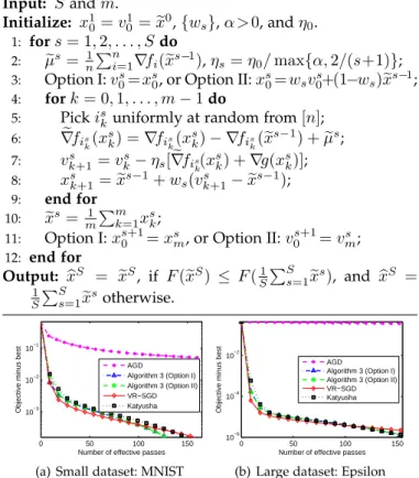
Theorem 5. Suppose Assumption 1 holds. Then the following inequality holds: E[F(bxS)−F(x∗)] ≤ 4(1−w1) w2 1(S+1)2 [F(xe0)−F(x∗)] + 2 mη0(S+1)2∥ x∗−ex0∥2.

Algorithm 3The momentum accelerated algorithm

Input: Sandm. Initialize: x1 0=v01=ex0,{ws},α >0, andη0. 1: fors= 1,2, . . . , Sdo 2: µes₌ 1 n ∑n i=1∇fi(xes−1),ηs=η0/max{α,2/(s+1)};

3: Option I:v₀s=xs₀, or Option II:xs₀=wsv0s+(1−ws)xes−1;

4: fork= 0,1, . . . , m−1do

5: Pickis

kuniformly at random from[n];

6: ∇efis k(x s k) =∇fis k(x s k)− ∇fis k(xe s−1_{) +µe}s_; 7: vs k+1=vsk−ηs[∇efis k(x s k) +∇g(xsk)]; 8: xs k+1=exs−1+ws(vks+1−xes−1); 9: end for 10: xes=_m1∑m_k=1xs_k; 11: Option I:xs₀+1=xs m, or Option II:v s+1 0 =vsm; 12: end for Output: xbS _{= xe}S_{, if F(ex}S_{) ≤ F(}1 S ∑S s=1xe s_{), and bx}S ₌ 1 S ∑S s=1xesotherwise. 0 50 100 150 10−3 10−2 10−1

Number of effective passes

Objective minus best

AGD Algorithm 3 (Option I) Algorithm 3 (Option II) VR−SGD Katyusha

(a) Small dataset: MNIST

0 50 100 150

10−6 10−4 10−2

Number of effective passes

Objective minus best

AGD Algorithm 3 (Option I) Algorithm 3 (Option II) VR−SGD Katyusha

(b) Large dataset: Epsilon

Fig. 2. Comparison of AGD [19], Katyusha [47], Algorithm3with Option I and II, and VR-SGD for solving logistic regression withλ= 0.

Choosing m= Θ(n), Algorithm3 with Option II achieves an ϵ-suboptimal solution (i.e.,E[F(bxS_)]−F(x∗_{)≤ε) using at most}

O(n√[F(xe0_{)−F(x∗)]/ε+}√_nL/ε∥xe0_−x∗∥)

iterations.

This theorem shows that the oracle complexity of

Algorithm 3 with Option II is consistent with that of

Katyusha [47], and is better than that of accelerated

deter-ministic methods (e.g., AGD [19]), (i.e.,O(n√L/ε)), which

are also verified by the experimental results in Fig. 2.

Our algorithm also achieves the optimal convergence rate

O(1/T2_{)for non-strongly convex functions as in [47], [48].}

Fig.2 shows that Katyusha and Algorithm 3 with Option

II have similar performance as Algorithms 2 and 3 with

Option I (η0=3/(5L)) in terms of number of effective passes.

Clearly, Algorithm3and Katyusha have higher complexity

per iteration than Algorithm 2. Thus, we only report the

results of VR-SGD (i.e., Algorithm2) in Section5.

4.4 Complexity Analysis

From Algorithm 2, we can see that the per-iteration cost

of VR-SGD is dominated by the computation of ∇fis

k(x s k), ∇fis k(xe s−1_{), and∇g(x}s

k)or the proximal update in (13). Thus,

the complexity isO(d), which is as low as that of SVRG [1]

and Prox-SVRG [33]. In fact, for some ERM problems, we

can save the intermediate gradients∇fi(xes−1)in the

com-putation of µes_{, which generally requires O(n) additional}

storage. As a result, each epoch only requires(n+m)

compo-nent gradient evaluations. In addition, for extremely sparse

data, we can introduce the lazy update tricks in [37], [71],

[72] to our algorithm, and perform the update steps in (12)

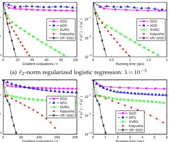
0 20 40 60 80 100 10−12 10−8 10−4 Gradient evaluations / n F (x s ) − F (x * ) SGD AGD SVRG Katyusha VR−SGD 0 0.5 1 1.5 2 10−12 10−8 10−4

Running time (sec)

F (x s ) − F (x * ) SGD AGD SVRG Katyusha VR−SGD

(a)ℓ2-norm regularized logistic regression:λ= 10−5

0 50 100 150 200 10−12 10−8 10−4 Gradient evaluations / n F (x s ) − F (x * ) SGD APG SVRG Katyusha VR−SGD 0 1 2 3 4 5 6 10−12 10−8 10−4

Running time (sec)

F (x s ) − F (x * ) SGD APG SVRG Katyusha VR−SGD

(b)ℓ1-norm regularized logistic regression:λ= 10−5 Fig. 3. Comparison of deterministic and stochastic methods on Adult.

rather than all dimensions. In other words, the per-iteration

complexity of VR-SGD can be improved fromO(d)toO(d′),

where d′ ≤d is the sparsity of feature vectors. Moreover,

VR-SGD has a much lower per-iteration complexity than existing accelerated stochastic variance reduction methods

such as Katyusha [47], which have more updating steps for

additional variables, as shown in (9a)-(9c).

5

E

R

In this section, we evaluate the performance of VR-SGD for solving a number of convex and non-convex ERM problems (such as logistic regression, Lasso and ridge regression), and compare its performance with several state-of-the-art

stochastic variance reduced methods (including SVRG [1],

Prox-SVRG [33], SAGA [30]) and accelerated methods, such

as Catalyst [39] and Katyusha [47]. Moreover, we apply

VR-SGD to solve other machine learning problems, such as ERM with non-convex loss and leading eigenvalue computation.

5.1 Experimental Setup

We used several publicly available data sets in the exper-iments: Adult (also called a9a), Covtype, Epsilon, MNIST, and RCV1, all of which can be downloaded from the

LIB-SVM Data website4_{. It should be noted that each sample of}

these date sets was normalized so that they have unit length as in [33], [35], which leads to the same upper bound on the Lipschitz constants Li, i.e., L=Li for all i= 1, . . . , n. As suggested

in [1], [33], [47], the epoch length is set to m = 2n for

the stochastic variance reduced methods, SVRG [1],

Prox-SVRG [33], Catalyst [39], and Katyusha [47], as well as

VR-SGD. Then the only parameter we have to tune by hand

is the learning rate,η. More specifically, we select learning

rates from{10j_,2.5×10j_,5×10j_,7.5×10j_,10j+1_{}, where}

j ∈ {−2,−1,0}. Since Katyusha has a much higher

per-iteration complexity than SVRG and VR-SGD, we compare their performance in terms of both the number of effective passes and running time (seconds), where computing a

4.https://www.csie.ntu.edu.tw/∼cjlin/libsvm/

single full gradient or evaluatingncomponent gradients is

considered as one effective pass over the data. For fair com-parison, we implemented SVRG, Prox-SVRG, SAGA, Cata-lyst, Katyusha, and VR-SGD in C++ with a Matlab interface, as well as their sparse versions with lazy update tricks, and performed all the experiments on a PC with an Intel i5-4570 CPU and 16GB RAM. The source code of all the methods is

available athttps://github.com/jnhujnhu/VR-SGD.

5.2 Deterministic Methods vs. Stochastic Methods

In this subsection, we compare the performance of stochastic methods (including SGD, SVRG, Katyusha, and VR-SGD)

with that of deterministic methods such as AGD [18], [19]

and APG [21] for solving strongly and non-strongly convex

problems. Note that the important momentum parameterw

of AGD isw= (√L−√µ)/(√L+√µ)as in [73], while that of

APG is defined as follows:wk = (αk−1)/αk+1for allk≥1

[21], whereαk+1= (1+

√

1+4α2

k)/2, andα1= 1.

Fig.3shows the the objective gap (i.e.,F(xs_)−F(x∗_{)) of}

those deterministic and stochastic methods for solvingℓ2

-norm andℓ1-norm regularized logistic regression problems

(see the Supplementary Material for more results). It can be seen that the accelerated deterministic methods and SGD have similar convergence speed, and APG usually performs slightly better than SGD for non-strongly convex problem-s. The variance reduction methods (e.g., SVRG, Katyusha and VR-SGD) significantly outperform the accelerated de-terministic methods and SGD for both strongly and non-strongly convex cases, suggesting the importance of vari-ance reduction techniques. Although accelerated determin-istic methods have a faster theoretical speed than SVRG for

general convex problems, as discussed in Section1.2, APG

converges much slower in practice. VR-SGD consistently outperforms the other methods (including Katyusha) in all the settings, which verifies the effectiveness of VR-SGD.

5.3 Different Choices for Snapshot and Starting Points

In the practical implementation of SVRG [1], both the

s-napshot xes _{and starting point x}s+1

0 in each epoch are set

to the last iterate xsm of the previous epoch (i.e., Option I

in Algorithm1), while the two vectors in [33] are set to the

average point of the previous epoch,_m1∑mk=1xsk(i.e., Option

II in Algorithm1). In contrast,exsandxs0+1in our algorithm

are set to _m1∑mk=1xsk and xsm (denoted by Option III, i.e.,

Option I5_{in Algorithm2), respectively.}

We compare the performance of the algorithms with the

three settings (i.e., the Options I, II and III listed in Table2)

for solving ridge regression and Lasso problems, as shown

in Fig.4(see the Supplementary Material for more results).

Except for the three different settings for snapshot and

start-ing points, we use the update rules in (12) and (13) for ridge

regression and Lasso problems, respectively. We can see that

the algorithm with Option III (i.e., Algorithm2with Option

I) consistently converges much faster than the algorithms with Options I and II for both strongly convex and non-strongly convex cases. This indicates that the setting of Option III suggested in this paper is a better choice than Options I and II for stochastic optimization.

5. As Options I and II in Algorithm2achieve very similar

TABLE 2

The three choices of snapshot and starting points for stochastic variance reduction optimization.

Option I Option II Option III

e xs_=xs m and x s+1 0 =xsm xes=m1 ∑m k=1xsk and x s+1 0 = 1 m ∑m k=1xsk exs= 1 m ∑m k=1xsk and x s+1 0 =xsm 0 5 10 15 20 25 30 10−12 10−8 10−4 Gradient evaluations / n F (x s ) − F (x * ) Option I Option II Option III 0 10 20 30 40 50 60 10−12 10−8 10−4 Gradient evaluations / n F (x s ) − F (x * ) Option I Option II Option III

(a) Ridge regression:λ= 10−5_{(left) and λ= 10}−6_(right)

0 5 10 15 20 25 30 10−12 10−8 10−4 Gradient evaluations / n F (x s ) − F (x * ) Option I Option II Option III 0 5 10 15 20 25 30 10−12 10−8 10−4 Gradient evaluations / n F (x s ) − F (x * ) Option I Option II Option III

(b) Lasso:λ= 10−4_{(left) and λ= 10}−5_(right)

Fig. 4. Comparison of the algorithms with Options I, II, and III for solving ridge regression and Lasso on Covtype. In each plot, the vertical axis shows the objective value minus the minimum, and the horizontal axis denotes the number of effective passes.

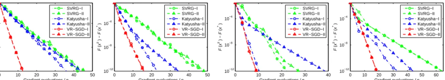
0 10 20 30 40 50 10−12 10−8 10−4 Gradient evaluations / n F (x s ) − F (x * ) SVRG−I SVRG−II Katyusha−I Katyusha−II VR−SGD−I VR−SGD−II 0 10 20 30 40 50 10−12 10−8 10−4 Gradient evaluations / n F (x s ) − F (x * ) SVRG−I SVRG−II Katyusha−I Katyusha−II VR−SGD−I VR−SGD−II

(a) Adult:λ= 10−3(left) andλ= 10−4(right)

0 10 20 30 40 10−12 10−8 10−4 Gradient evaluations / n F (x s ) − F (x * ) SVRG−I SVRG−II Katyusha−I Katyusha−II VR−SGD−I VR−SGD−II 0 10 20 30 40 50 60 10−12 10−8 10−4 Gradient evaluations / n F (x s ) − F (x * ) SVRG−I SVRG−II Katyusha−I Katyusha−II VR−SGD−I VR−SGD−II

(b) Covtype:λ= 10−5(left) andλ= 10−6(right)

Fig. 5. Comparison of SVRG [1], Katyusha [47], VR-SGD and their proximal versions for solving ridge regression problems. In each plot, the vertical axis shows the objective value minus the minimum, and the horizontal axis is the number of effective passes over data.

5.4 Common SG Updates vs. Prox-SG Updates

In this subsection, we compare the original Katyusha

algo-rithm in [47] with the slightly modified Katyusha algorithm

(denoted by Katyusha-I). In Katyusha-I, only the following two update rules are used to replace the original proximal

stochastic gradient update rules in (9b) and (9c).

ys_k+1=ys_k−η[∇efik(xsk+1) +∇g(x s k+1)], z_ks₊₁=xs_k+1−[∇efik(x s k+1) +∇g(x s k+1)]/(3L). (16)

Similarly, we also implement the proximal versions6 for

the original SVRG (called SVRG-I) and VR-SGD (denoted by VR-SGD-I) methods, and denote their proximal variants by SVRG-II and VR-SGD-II, respectively. In addition, the original Katyusha is denoted by Katyusha-II.

Fig. 5 shows the performance of Katyusha-I and

Katyusha-II for solving ridge regression on the two popular data sets: Adult and Covtype. We also report the results of SVRG, VR-SGD, and their proximal variants. It is clear that Katyusha-I usually performs better than Katyusha-II

(i.e., the original Katyusha [47]), and converges significantly

faster in the case when the regularization parameter is10−4

or 10−6. This seems to be the main reason why Katyusha

has inferior performance when the regularization parameter

is relatively large, as shown in Section 5.6.1. In contrast,

VR-SGD and its proximal variant have similar performance,

6. Here, the proximal variant of SVRG is different from Prox-SVRG [33], and their main difference is the choices of both the snapshot point and starting point. That is, the two vectors of the former are set to the last iteratexs

m, while those of Prox-SVRG are set to the average

point of the previous epoch, i.e.,_m1∑mk=1xsk.

0 5 10 15 20 10−12 10−8 10−4 Gradient evaluations / n F (x s ) − F (x * ) SVRG++ VR−SGD VR−SGD++ (a)λ= 10−5 0 10 20 30 40 10−12 10−8 10−4 Gradient evaluations / n F (x s ) − F (x * ) SVRG++ VR−SGD VR−SGD++ (b)λ= 10−6

Fig. 6. Comparison of SVRG++ [43], VR-SGD and VR-SGD++ for solv-ing logistic regression problems on Epsilon.

and the former slightly outperforms the latter in most cases (similar results are also observed for SVRG vs. its proximal variant). This suggests that stochastic gradient update rules

as in (12) and (16) are better choices than proximal update

rules as in (10), (9b) and (9c) for smooth objective functions.

We also believe that our new insight can help us to design accelerated stochastic optimization methods.

Both Katyusha-I and Katyusha-II usually outperform SVRG and its proximal variant, especially when the

reg-ularization parameter is relatively small, e.g., λ = 10−6_.

Moreover, it can be seen that both VR-SGD and its prox-imal variant achieve much better performance than the other methods in most cases, and are also comparable to Katyusha-I and Katyusha-II in the remaining cases. This further verifies that VR-SGD is suitable for various large-scale machine learning.