ISTANBUL TECHNICAL UNIVERSITY GRADUATE SCHOOL OF SCIENCE ENGINEERING AND TECHNOLOGY
M.Sc. THESIS
SPARSE CODING BASED ENSEMBLE CLASSIFIERS COMBINED WITH ACTIVE LEARNING FRAMEWORK FOR DATA CLASSIFICATION
Göksu TÜYSÜZOĞLU
Department of Computer Engineering Computer Engineering Programme
Department of Computer Engineering Computer Engineering Programme
ISTANBUL TECHNICAL UNIVERSITY GRADUATE SCHOOL OF SCIENCE ENGINEERING AND TECHNOLOGY
SPARSE CODING BASED ENSEMBLE CLASSIFIERS COMBINED WITH ACTIVE LEARNING FRAMEWORK FOR DATA CLASSIFICATION
M.Sc. THESIS Göksu TÜYSÜZOĞLU
(504131520)
Thesis Advisor: Asst. Prof. Dr. Yusuf YASLAN
Bilgisayar Mühendisliği Anabilim Dalı Bilgisayar Mühendisliği Programı
İSTANBUL TEKNİK ÜNİVERSİTESİ FEN BİLİMLERİ ENSTİTÜSÜ
VERİ SINIFLANDIRMA İÇİN AKTİF ÖĞRENME ÇERÇEVESİ İLE BİRLEŞTİRİLMİŞ AYRIK KODLAMA TABANLI SINIFLANDIRICI
TOPLULUKLARI
YÜKSEK LİSANS TEZİ Göksu TÜYSÜZOĞLU
(504131520)
Tez Danışmanı: Yrd. Doç. Dr. Yusuf YASLAN
v
Thesis Advisor : Asst. Prof. Dr. Yusuf YASLAN ... İstanbul Technical University
Göksu TÜYSÜZOĞLU, a M.Sc. student of ITU Graduate School of Science Engineering and Technology student ID 504131520, successfully defended the thesis entitled “SPARSE CODING BASED ENSEMBLE CLASSIFIERS COMBINED WITH ACTIVE LEARNING FRAMEWORK FOR DATA CLASSIFICATION”, which she prepared after fulfilling the requirements specified in the associated legislations, before the jury whose signatures are below.
Jury Members : Assoc. Prof. Dr. Sanem SARIEL ... İstanbul Technical University
Asst. Prof. Dr. Tolga ENSARİ ... İstanbul University
Date of Submission : 2 May 2016 Date of Defense : 10 June 2016
vii
ix FOREWORD
This thesis was written for my Master degree in Computer Engineering at Istanbul Technical University. I would like to thank my supervisor Asst. Prof. Dr. Yusuf Yaslan for giving me valuable advice, guidance and support always when needed. Other important persons considering my thesis are Nazanin Moarref and all the professors in the Department of Computer Engineering at Istanbul Technical University whom I like to give my special thanks for giving me an opportunity to share their knowledge and the best available information.
Finally, I like to show my gratitude to thank my family and also my friends and colleagues, Gamze Doğan, Beyza Eken, Mine Yasemin and Kübra Cengiz for their constant support and encouragement to boost my positive energy and motivation throughout the process of writing my thesis.
May 2016 Göksu TÜYSÜZOĞLU
xi TABLE OF CONTENTS
Page
FOREWORD ... ix
LIST OF TABLES ... xv
LIST OF FIGURES ... xvii
SUMMARY ... xix
ÖZET...xxi
1. INTRODUCTION ... 1
1.1 Purpose of Thesis ... 3
1.2 Literature Review ... 4
1.3 Outline of the Thesis ... 8
2. METHODOLOGY ... 9
2.1 Dictionary Learning and Sparse Signal Approximation ... 9
2.2 Support Vector Machines ... 12
2.2.1 Non-separable case ... 14
2.3 Ensemble Learning ... 16
2.3.1 Random subspace ensemble learning ... 18
2.3.2 Bagging ... 19
2.4 Active Learning ... 19
3. THE PROPOSED METHOD ... 23
3.1 Dictionary Ensembles Using Random Subspaces and Bagging ... 23
3.2 Active Learning Based Data Classification Using Dictionary Ensembles ... 24
4. MATERIALS AND EXPERIMENTAL SETUP ... 29
5. EXPERIMENTAL RESULTS ... 31
5.1 Performance Analysis Based on Classification Accuracies ... 31
5.2 Friedman Test ... 34
5.3 Wilcoxon Signed Rank Test ... 38
6. CONCLUSIONS AND RECOMMENDATIONS ... 43
REFERENCES ... 45
xiii ABBREVIATIONS
ARDL : Active Random Subspace Dictionary Learning ARSVM : Active Random Subspace Support Vector Machines ABDL : Active Bagging Dictionary Learning
ABSVM : Active Bagging Support Vector Machines BDL : Bagging Dictionary Learning
BSVM : Bagging Support Vector Machines DL : Dictionary Learning
RDL : Random Subspace Dictionary Learning RS : Random Subspace Feature Selection
RSVM : Random Subspace Support Vector Machines SVM : Support Vector Machines
xv LIST OF TABLES
Page
Table 2.1 : The pseudo code of random subspace ensemble learning. ... 18
Table 2.2 : The pseudo code of bagging. ... 20
Table 3.1 : The pseudocode of the proposed ensemble methods. ... 24
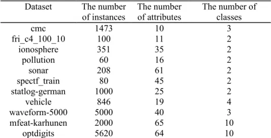
Table 4.1 : Properties of the datasets used in the experimental results. ... 29
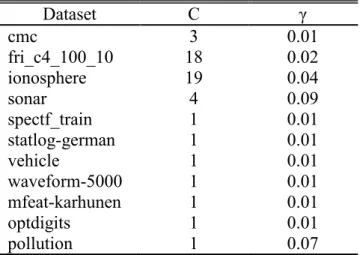
Table 5.1 : SVM parameters for each dataset. ... 31
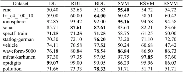
Table 5.2 : Classification accuracies of the classifiers DL and SVM along with their ensembles. ... 32
Table 5.3 : Active learning classification results based on dictionary learning using random subspace ensemble. ... 33
Table 5.4 : Active learning classification results based on support vector machine using random subspace ensemble. ... 33
Table 5.5 : Active learning classification results based on dictionary learning using bagging ensemble. ... 33
Table 5.6 : Active learning classification results based on support vector machine using bagging ensemble. ... 34
Table 5.7 : The last iteration accuracies of active learning methods. ... 35
Table 5.8 : Friedman test rankings of DL and SVM along with their respective ensembles. ... 39
Table 5.9 : Friedman test rankings of different active learning iterations for random subspace dictionary learning model. ... 39
Table 5.10 : Friedman test rankings of different active learning iterations for random subspace support vector machines model. ... 40
Table 5.11 : Friedman test rankings applied on the last iteration of active learning methods. ... 40
Table 5.12 : Application of Wilcoxon signed rank test on the pairs of DL/RDL and DL/SVM algoritms. ... 41
Table 5.13 : Application of Wilcoxon signed rank test on the pairs of the last iteration accuracies of the active learning models. ... 42
xvii LIST OF FIGURES
Page
Figure 2.1 : Iterative dictionary learning framework. ... 12
Figure 2.2 : Two class data points linearly separable by a hyperplane. ... 13
Figure 2.3 : An example of linearly separable (left) and non-separable (right) SVM ... 15
Figure 2.4 : Ensemble learning framework. ... 17
Figure 2.5 : Active learning framework. ... 21
Figure 3.1 : Framework of the proposed ensemble dictionary learning models. ... 26
xix
SPARSE CODING BASED ENSEMBLE CLASSIFIERS COMBINED WITH ACTIVE LEARNING FRAMEWORK FOR DATA CLASSIFICATION
SUMMARY
Nowadays, along with the need for classification algorithms in various areas concerning machine learning such as text classification, image categorization, audio and music genre classification, new classifier models are developed and works for improving the existing ones increasingly go on. In this direction, as dictionary learning algorithm which represents signals or each problem instance at hand with sparse linear combinations of basis elements of a dictionary is also utilized in data classification and clustering, it is used in signal, image, audio and video processing applications.
In the dictionary learning model, which sparse coding and dictionary update steps are practiced and this process continues until a predetermined convergence level is attained in an iterative fashion. The main purpose is to obtain the framework of a dictionary that provides the sparsest representation while decreasing the reconstruction error.
The process where a number of classifiers are modeled and decisions from each one produce a single output by a combination rule is known as ensemble learning. In literature, ensemble learning algorithms is performed both in feature subspace and instance subspace. Random subspace feature selection and bagging are the mostly applied ensemble learning methods in feature subspace and in instance subspace respectively.
On the other hand, possibility of access to huge amount of unlabeled data has been increased along with getting easy access to data. Active learning, which is proposed for this type of problems, is a learning method in which the most informative instances from the unlabeled data are chosen, then labeled by an oracle and after then added to the training set.
At the stage of establishing the active learning framework, evaluation of the unlabelled data and how to select the most informative ones among them is an important question. One of the easiest ways is to select the signals where the classifier is least certain about their class labels in the query phase. This method is known as uncertainty sampling. One of the most popular maximal uncertainty sampling techniques is based on entropy. The more entropy in the distribution, the more uncertain the choice of class label for that data value, and the more informative that query would be.
In the first stage of this study, dictionary learning is applied in combination with random subspace feature selection and bagging ensemble models. Then, comparisons of the experimental results with support vector machine, which is one of the best classifier models, and its ensemble combinations are maintained.
According to ten-fold cross validation experimental results obtained on eleven datasets from various area of specialization taken from UCI machine learning
xx
repository and OpenML, dictionary learning based ensemble classifiers, especially BDL algorithm, present more successful classification performance than both of SVM and its classifier ensembles. Considering the experimental results, BDL outperforms other applied methods in 4 out of 11 datasets and in 2 datasets it performs the best with the other two methods DL and RDL. As a consequence, we can infer that randomly selecting instance subspaces while constructing dictionary models has a positive effect on the classification accuracy of the established methods.
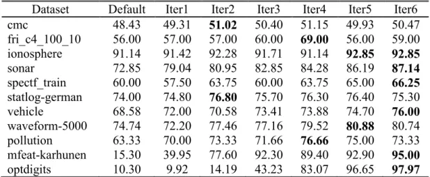
In the second stage, all the dictionary base proposed methods and support vector machine counterparts are combined with active learning framework in which the most informative unlabelled training instances are labeled and integrated into the labeled training set in each learning iteration. While predicting the class labels of the test examples, the decision is made applying majority voting. After examining the experimental results, it is evident that classification accuracy mostly increases as the number of iterations goes up by the selection of training instances intelligently. Regarding to the best results obtained for each dataset by applied models, while ARDL outperforms ARSVM's classification performance, ABSVM succeeds better results than ABDL.
After obtaining the experimental results, an important part to handle is to measure the significance of the hypotheses which put forward the equivalency of the applied methods based on classification accuracies. In this direction, Friedman and Wilcoxon signed rank test results were obtained both for the ensemble learning part and methods under active learning framework. According to outcomes from the Friedman significance tests, ARDL, ARSVM, ABDL and ABSVM do not perform equivalently regarding to the best results obtained for each dataset.
On the other hand, Friedman significance tests and Wilcoxon signed rank tests applied to the accuracy results in the last iteration of active learning models are resulted in similar classification performance in the predetermined confidence interval. In the last part, Friedman test is practiced among DL and SVM classifiers and their ensemble models. Because there is an equivalency between classification performance differences, Wilcoxon signed rank test is applied to see pairwise model differences. As a result, DL/RDL, DL/BDL and SVM/BSVM pairs have significant differences while the other model couples performs in the same manner.
xxi
VERİ SINIFLANDIRMA İÇİN AKTİF ÖĞRENME ÇERÇEVESİ İLE BİRLEŞTİRİLMİŞ AYRIK KODLAMA TABANLI SINIFLANDIRICI
TOPLULUKLARI ÖZET
Günümüzde metin sınıflandırma, görüntü kategorizasyonu, ses ve müzik türü sınıflandırması gibi makine öğrenmesi konusunda farklı disiplinlerden pek çok alanda sınıflandırma algoritmalarına olan ihtiyaç bir hayli artmıştır. Bu amaçla yeni sınıflandırıcı modeller geliştirilmekte ve mevcut algoritmaları da iyileştirme çalışmaları çoğalarak devam etmektedir.
Sinyalleri ya da elimizde bulunan her bir problem örneğini bir sözlüğün temel elemanlarının ayrık doğrusal kombinasyonları olarak temsil etmekte olan sözlük öğrenme algoritmasından da bu doğrultuda veri sınıflandırma ve kümeleme alanlarında çokça faydalanılmakta olup sinyal, görüntü, ses ve video işleme uygulamalarında kullanılmaktadır.
İki aşamada gerçekleştirilen sözlük öğrenmesi modelinde ayrık kodlama ve sözlük güncelleme adımları uygulanmakta ve belirli bir yakınsama elde edene kadar bu süreç iteratif olarak devam etmektedir. Ana amaç, yeniden yapılandırma hatasını azaltarak en çok ayrık gösterimi veren sözlük yapısını elde etmektir.
Birçok sınıflandırıcının modellendiği ve her birinden gelen kararların birleştirilerek tek bir çıktı ürettiği süreç topluluk öğrenme olarak bilinir. Literatürde makine öğrenmesi uygulamalarının çoğunda sınıflandırıcı topluluklar tek sınıflandırıcı yöntemlerinden daha iyi başarım gösterebilmektedir. Topluluk öğrenme algoritmaları hem örnek hem de öznitelik alt uzaylarında uygulanabilmektedir. Random subspace algoritması öznitelik uzayında ve bagging algoritması da örnek uzayında en çok uygulanan topluluk öğrenme yöntemlerindendir.
Öte yandan veriye erişimin kolaylaşması ile birlikte çok büyük miktarda etiketsiz veriye erişim imkânı doğmuştur. Bu tür problemler için sunulan aktif öğrenme, etiketi bilinmeyen veriler içerisinden en çok bilgi verici örnekleri seçip uzmanlar tarafından etiketleyerek eğitim kümesi içine katan bir öğrenme yöntemidir.
Aktif öğrenme yapısının kurulması aşamasında etiketsiz verilerin değerlendirilip içlerinden en bilgi verici olanlarının nasıl seçileceği önemli bir sorudur. En kolay yollardan biri, örnekleri sorgulayarak sınıflandırıcı modelin sınıf etiketi konusunda en az emin olduğu sinyallerin seçilmesidir ve bu yöntem belirsizlik örnekleme (uncertainty sampling) olarak bilinir. Belirsizlik örnekleme teknikleri içinde en popüler olanlarından biri düzensizlik hesabını temel alır. Bir dağılımda ne kadar fazla düzensizlik varsa, o veri için sınıf etiketi seçimi de o derecede kararsızlık içerir ve sorgulama da o kadar bilgi verici olur.
Bu çalışmanın ilk aşamasında sözlük öğrenme modeli, sınıflandırıcı topluluklarından random subspace feature selection ile öznitelik alt uzayında ve bagging ile örnek alt uzayında birleştirilerek uygulanmış ve bu sınıflandırıcılar Random Subspace Dictionary Learning (RDL) ve Bagging Dictionary Learning (BDL) olarak
xxii
adlandırılmıştır. Deneysel sonuçlarda önerilen yöntemlerin sınıflandırma başarımları en iyi sınıflandırıcı yöntemlerden biri olan destek vektör makinesi (Support Vector Machines - SVM) ve topluluk öğrenme tabanlı kombinasyonları (Random Subspace Support Vector Machines (RSVM) ve Bagging Support Vector Machines (BSVM)) ile birlikte karşılaştırılmıştır.
UCI makine öğrenmesi veri havuzundan ve OpenML' den alınan çeşitli alanlardan on bir farklı veri kümesi üzerinde elde edilen on kat çapraz sağlama deney sonuçlarına göre sözlük öğrenme tabanlı sınıflandırıcı toplulukları, özellikle de BDL algoritması, hem destek vektör makineleri hem de sınıflandırıcı topluluklarıyla birleştirilmiş modellerine göre daha başarılı sonuçlar ortaya koymuştur.
Sınıflandırma başarımlarına bakıldığında, en başarılı yöntem olan BDL 11 veri kümesinin 4 tanesinde DL, RDL SVM, BSVM ve RSVM sınıflandırıcılarından üstün gelmekte, 2 tanesinde ise DL ve RDL ile en sonuçları elde etmektedir. Bu noktada örnek altuzaylarının rastgele seçilmesiyle oluşturulan sözlük modellerinin sınıflandırma başarımına olan pozitif etkisi gözlemlenmiştir.
İkinci aşamada ise uygulanan yöntemlerin her biri aktif öğrenme yapısı içerisinde kullanılmış, elde bulunan her bir sınıf için bir sözlük öğrenilerek, her iterasyonda en bilgi verici etiketsiz örnekleri etiketleyerek eğitim kümesine ekleme işlemi uygulanmıştır. Test aşamasında her yeni örnek için sınıf etiketi sözlük topluluklarının çoğunluğuna bakılarak atanmıştır.
İlk aşamada eldeki eğitim kümesinin %20'si alınarak hem sözlük tabanlı hem de destek vektör makinesi tabanlı sınıflandırıcı toplulukları modellenmiş, sonraki altı iterasyonda geriye kalan etiketsiz veriler içerisindeki en çok bilgi verici %10 örneğin düzensizlik hesabı dikkate alınarak seçilmesiyle eğitim kümesi güncellenmiştir. Böylelikle iterasyon sayısı arttıkça sınıflandırma başarımı da çoğunlukla artışa geçmiş, örneklerin akıllıca seçilmesiyle oluşturulan eğitim kümesi bu sonuçlarda etkili olmuştur.
Test sonuçlarında her bir veri kümesi için elde edilen en başarılı sonuçlar dikkate alınırsa, rastgele öznitelik seçimiyle oluşturulan sınıflandırıcı topluluklarına bakıldığında önerilen ARDL yönteminin ARSVM yönteminden daha başarılı olduğu görülmüştür. Örneklerin rastgele seçilmesiyle oluşturulan sınıflandırıcı toplulukları kullanıldığında ise ABSVM yöntemi ABDL yönteminden daha üstün gelmiştir. Deney sonuçlarının elde edilmesinden sonra ilgilenilmesi gereken önemli bir nokta da uygulanan yöntemlerin sınıflandırma başarımları açısından birbirine denkliğini öne süren hipotezlerin anlamlılığının ölçülmesidir. Bu doğrultuda, Friedman test ve Wilcoxon signed rank test sonuçlarına bakılmıştır. Friedman anlamlılık testinden gelen çıktılara göre aktif öğrenme altında iterasyon bazında uygulanan metotlar için en iyi sonuçlar dikkate alındığında görülen odur ki sıfır hipotezi (H0) kabul
edilmemelidir, başka bir deyişle uygulanan yöntemler gösterdikleri performans açısından eşdeğer değildirler.
Aktif öğrenme algoritmalarının son iterasyonlarında elde edilen başarımlar için de Friedman ve Wilcoxon signed rank testleri uygulanmıştır. Her iki test sonucunda da model çiftlerinin eş sınıflandırma performansları sundukları kanısına varılmıştır. Öte yandan pasif öğrenme kısmında uygulanan yöntemler de Friedman testiyle incelendiğinde eşdeğer oldukları görülmüştür. Bunun ardından, hangi metot çiftlerinin kendi aralarında denk performans sunup sunmadıkları sorusuna çözüm bulmak amacıyla Wilcoxon signed rank test uygulanmıştır. Sonuçlara göre DL/RDL,
xxiii
DL/BDL ve SVM/BSVM metot çiftleri sınıflandırma performansı olarak eşdeğer değildirler, diğer yöntemler ise denk sayılabilir.
1 1. INTRODUCTION
Nowadays, a plenty of latent information are available in databases to be exploited for intelligent decision making. These databases generally contain data that is related to a specific category or class. When data samples come with class labels, they are called training data which can be used to train a model for predicting the labels of new unseen data samples that are called test sets. This process is called classification and it is a concept to investigate to which class a new data point should belong under favour of using the training data. Han, Kamber and Pei (2011) express the idea as "Classification is the process of finding a model (or function) that describes and distinguishes data classes or concepts, for the purpose of being able to use the model to predict the class of objects whose class label is unknown" (p. 24). The process is known as supervised learning, because a model is formed using predefined training data, which in fact is used as a supervisor to classify new test examples.
There are lots of domains where classification takes place such as text categorization, optical character recognition, fraud detection, market segmentation, face detection, classification of proteins. In order to construct a classifier model, many machine learning algorithms have been developed and as new researches are presented, many others arise day-to-day. Support vector machines, decision trees, naive bayes, nearest neighbor, multilayer perceptron and logistic regression are some examples among the most popular classification algorithms. In order to obtain a good classification accuracy one also needs to have a good feature representation. In literature there is a vast amount of research to represent the features in other dimensional spaces to improve the classification performance such as kernels (Lu et al, 2003), wavelet transformation (Van de Wouwer et al, 1999), frequency representation of time domain signals (Sejdić et al, 2009).
A number of media types such as imagery, video and acoustic can be sparsely represented by applying transform-domain methods (Elad, 2010). A lot of significant tasks related to such media can be handled finding sparse solutions to underdetermined systems of linear equations. Regarding this issue, sparse coding and
2
dictionary learning have recently aroused much interest by representing each problem instance as linear combinations of basis elements. These elements are called atoms and they compose a dictionary.
One of the major application areas for dictionary learning is in data representation and classification. It has been applied in many problem areas such as signal processing applications (the joint analysis of correlated signals like audio-visual signals and stereo images) (Tošić and Frossard, 2011), texture segmentation (Sprechmann and Sapiro, 2010), music genre classification (Yeh and Yang, 2012) and saliency detection (Zhu, Chen and Zhao, 2014). The basic model for classification is created via generating one sub-dictionary for each category to represent the instances of the respective class and then combining them to reach a unique dictionary. The resulting dictionary base is used as a classifier that assigns a class label which has the least reconstruction error and the sparsest representation. Let us think of a scenario in which a group of doctors diagnose a certain disease for a patient. It is clear that the diagnosis is more reliable when the majority of doctors make the same decision on the patient's disease compared to the decision taken by the minority. From data classification perspective, in order to classify new test examples in a more accurate way, more than one classifier decisions can be integrated into the system and an agreement can be made on the final decision. This learning strategy is called ensemble learning and it is constituted by the combination of predictor/classifier model outputs, which produces a final decision for an unseen data point.
Ensemble learning methods are used for classification problems as well as regression. Classifier ensembles can be obtained either in feature space, instance space or classifier level. Boosting, bootstrap aggregating (bagging), stacking, random subspace feature selection, random forests and adaboost are among the most applied ensemble learning methods (Polikar, 2006).
Bagging is an instance-based ensemble learning method which generates subspaces of instances by applying random selection method with replacement. Each ensemble classifier produces a decision and the final prediction is their combined output. On the other hand, random subspace feature selection is a feature-based counterpart of bagging model, where a sub-group of features are randomly selected with
3
replacement to form ensemble classifiers. Taking advantage of the strengths of these two ensemble learning methods, classification problems can be solved more accurately and the variance of the individual classifiers are reduced.
Obtaining labeled training examples for classification problems is an expensive task while a massive chunk of unlabelled data is available to process. For instance, let us think of a case where we want to predict which web pages a person can find interesting. In order to do this, we need the data of web pages which were marked as favourite by this person. The more we know about the labeling information, we can predict better and present more appropriate pages to recommend. On the other side, people are generally not willing to hand-label all the pages they like even if there are a lot. Active learning is a largely used framework for these kind of situations. It has the ability to choose the most informative unlabeled examples automatically for human annotation. Liere and Tadepalli (1997) state the concept as "Active learning in its most general sense refers to any form of learning wherein the learning algorithm has some degree of control over the examples on which it is trained" (p. 591).
Up to the present, active learning framework has been applied with many different classifiers for text classification, image retrieval, advertisement removal (Sun and Hardoon, 2010), visual object detection (Abramson and Freund, 2004), natural language processing (Olsson, 2009) etc. To the best of our knowledge, active learning has not been applied as a classifier in active learning framework. In this study, dictionary learning is used as a base classifier for active learning and active learning’s intelligent selection strategy is used to enhance the training set by choosing the most informative examples.
1.1 Purpose of Thesis
The aim of the thesis is to introduce a number of models for data classification which are generated by sparse coding based ensemble classifiers combined with active learning framework. The proposed models are examined under three main headings: dictionary learning, ensemble learning and active learning framework.
In order to represent the input data using as few components as possible, dictionary learning is proposed as a learning model for an effective representation. Exploring
4
a sparse representation of the input data in the form of a linear combination of basis elements and also discovering those basis elements (i.e. atoms of a dictionary) themselves is the main purpose of dictionary learning.
Another remarkable point for this thesis is to show the effect of ensemble learning methods on the proposed classifiers. Random subspace feature selection and bagging are selected as appropriate ensemble learning methods to boost the prediction ability of dictionary learning model. On the other side, comparisons with support vector machines, which is one of the state-of-the-art algorithms, and its classifier ensembles are also presented. Toward this goal, experiments are conducted on datasets with different number of features/instances from various scopes.
Other point of purpose on the following sections is to introduce active learning framework and integrate it into ensemble dictionary learning model. It helps performing classification in cases where few number of labeled and huge number of unlabeled training instances are available. Entropy is employed as an uncertainty sampling technique for pool-based active classifier models.
As the final contribution of this paper, several significance tests are demonstrated to detect differences in treatments across multiple test attempts. For this purpose, non-parametric Friedman tests are applied to the classification accuracies of the proposed methods.
1.2 Literature Review
In literature, dictionary learning and sparse coding have been applied in diverse areas such as signal, image, audio and video processing applications for dimensionality reduction (Schnass and Vandergheynst, 2008; Tošić and Frossard 2011), denoising (Elad and Aharon, 2006), image restoration (Mairal et al, 2008), and image compression (Bryt and Elad, 2008).
As dictionary learning doesn’t require estimating class distributions or computing margin between classes, it is also used for data classification and clustering applications where the feature vectors are computed as linear combinations of basis elements of a dictionary. Sapiro and Sprechmann (2010) developed a clustering framework in which a set of dictionaries are built for every cluster found in a given dataset. According to the proposed approach, dictionaries are formed by choosing the
5
ones which provide the best representation of the signals in a cluster and giving the sparsest solution. Besides, three standard datasets, the MNIST and USPS which are composed of handwritten digits and ISOLET which includes audio features from 150 speakers were used to show the discriminative aspect of dictionary learning model. The experimental results showed that the proposed dictionary learning model provides remarkable classification performance comparable with other sophisticated classification algorithms such as SVM and k-NN in terms of reconstruction and discrimination power.
On the subject of music genre classification, Yeh and Yang (2012) developed a technique enforced by dictionary learning to summarize short-time features (codebook) of recorded music over time, where codebook represents dictionary base. Dictionary base is made up of sub-dictionaries, one for each class to represent the characteristics of the instances in these classes. Other existing codebook generation methods such as conventional VQ-based and exemplar-based methods were compared with the proposed dictionary based method. The proposed method was shown superior to others on two benchmark datasets, GTZAN composed of clips covering ten genres and ISMIR2004Genre including songs covering six genres using just the log-power spectrogram as the local feature descriptor.
Tošić and Frossard (2011) presented dictionary learning and sparse approximation as a dimensionality reduction tool to find a representation adaptive to the proper inference of causes of the observed data. In addition, supervised dictionary learning was examined in a face recognition application by using the discriminative power of the sparse representation. The incoherency between the subspaces which represent data in different classes was taken into consideration.
Recently, ensemble methods have been used to improve the classification accuracy of single classifiers. Ensemble classifiers are created using the outputs of multiple classifiers that are trained on different training datasets created by various data resampling procedures or trained on a single training dataset by selecting different classifier parameters or classifiers.
Polikar (2006) reviewed ensemble based strategies such as bagging and its variations, boosting models, stack generalization etc. by emphasizing their importance in decision making process while dealing with classification problems.
6
Why we tend to prefer applying ensemble learning methods instead of single classifiers is explained from various perspectives such as reducing the risk of inaccurate predictions of a single model, ability of handling large volumes of data and easily applying divide and conquer technique in problems with complex decision boundaries.
Random subspace is one of the well-known ensemble learning methods. It was firstly introduced to construct a decision tree classifier by randomly chosen subspaces of the components of the feature vector (Ho, 1998). According to the applied selection strategy to form random subspaces, a number of different feature selection techniques has been proposed such as Univariate search technique (Chow et al, 2001), Base-pair selection (Bo and Jonassen, 2002), Forward selection (Bo and Jonassen, 2002), Recursive Feature Elimination, and Liknon.
Lai, Reinders and Wessels (2006) introduced an ensemble strategy in feature space by incorporating informativeness of features as a selection strategy in the construction of each subspace. Applied multivariate feature selection technique, Random Subspace Method, initially selects features randomly from the original feature space and then, a multivariate search technique, either Liknon or Recursive Feature Elimination, takes place in this reduced feature space by retrieving the informative features. This procedure is applied iteratively by covering the large portions of the original features. According to the experimental results which were carried out in artificial datasets, ensemble based random subspace model provides robustness and a powerful classification performance especially in small sample size problems. Many other studies have been made by applying random subspace ensemble for functional magnetic resonance imaging (fMRI) classification (Kuncheva et al, 2010), the bio-molecular diagnosis of malignancies (Bertoni, 2005) and bankruptcy prediction and credit scoring (Nanni and Lumini, 2009) etc.
Bagging is another ensemble learning strategy which uses randomly selected instance subspaces. There are various studies applying bagging for solving credit scoring and bankruptcy prediction (West, 2005), optical character recognition (Mao, 1998) and day-ahead electricity price prediction (Tian and Meng, 2010). Recently, Zhu et al. (2014) combined ensemble learning with dictionary learning model in order to detect visually salient regions of an image. Instead of modeling a universal dictionary, the developed bagging based dictionary learning framework (EDL) is
7
constructed by applying random selection of image samples in order to train dictionaries independently for each subspace. In this way, more flexible multiple sparse representations are obtained for each of the image patches. A reconstruction residual based model for atom reduction over the learned dictionary is presented to further boost the distinctness of salient patch from the one of background. The resulting decision is made upon considering the outputs from each ensemble subspace. To the best of our knowledge there isn’t any paper that applies dictionary learning as base classifier for random subspace and bagging ensembles.
The possibility of access to huge amount of data has been increased along with getting easy access to data. On the other hand, the majority of the available data is mostly unlabeled in other words we do not have enough information about its class/category label. Active learning, which is proposed for this type of problems, is a learning method in which the most informative instances from the unlabeled data are chosen, then labeled by an oracle and after then added to the training set to be used in the model construction of classification.
Active learning can be categorized by its way of synthesizing queries either by stream-based (Cohn et al, 1994), pool-stream-based (Lewis and Gale, 1994) or query synthesis (Angluin, 1988) methods. In this work, the focus is on pool-based active learning in which a large pool of instances are sampled then the base classifier chooses the best query to be labeled. There are numerous number of studies applying pool-based active learning for different purposes such as in the application of cancer diagnosis
(Liu, 2004), image classification (Zhang and Chen, 2002) and speech recognition
(Tur et al, 2005).
Tong and Koller (2001) performed classification using SVM under the active learning framework in a text classification problem to determine which pre-defined topic a given text document belongs to. In the active learning part, some number of unlabeled instances are selected and added to the training set after learning its class label using one type of pool based active learning strategy. Three query strategies that split the version space into equal parts was proposed and they were shown to outperform standard passive learning counterparts.
Sun (2010) developed an active learning model which takes the correlation values between features of different views under a multi-view setting. He applied canonical
8
correlation analysis to select the most informative instances to integrate them into the training phase in the further iterations. According to the proposed approach, it is assumed that one example per class is labeled. The experiments were conducted on text classification, advertisement removal and content-based image retrieval and it was showed that the proposed active learning model has superiority over the general random selection approach for labeling.
Xu et al. (2014) performed active learning for dictionary construction by choosing the most informative examples using the reconstruction and classification error as the query strategy. The selected instance is only used during the dictionary update step. According to the experimental results conducted on a number of datasets from UCI Machine Learning Repository and face recognition dataset, active dictionary learning with small size dictionary can achieve comparable performance with other machine learning methods.
1.3 Outline of the Thesis
The rest of the thesis is organized as follows: The next chapter introduces the applied methodology. In the first step, sparse signal representation, dictionary learning and support vector machines models are explained. The following step of Chapter 2 is devoted to the ensemble learning methods in general and provides detailed knowledge on random subspace feature selection and bagging ensemble classifiers. Furthermore, active learning framework is stated by expanding different sampling scenarios used throughout literature. In the next chapter, sparse coding based ensemble classifiers combined with active learning framework is proposed. Chapter 4 discusses datasets which have been used and toolboxes managed to obtain dictionary learning model and support vector machines classifiers. In Chapter 5 experimental results achieved and significance tests applied are explained while Chapter 6 concludes the thesis with a summary of key lessons learnt.
9 2. METHODOLOGY
2.1 Dictionary Learning and Sparse Signal Approximation 2.1.1 Sparse signal approximation
Sparse representations of signals have received a great deal of attentions in recent years. Sources of data such as voice signals, images, radar images or heart signals etc. carry overwhelming amounts of data in which relevant information is often more difficult to find than a needle in a haystack. In this direction, having a sparse representation plays a fundamental role in processing signals faster and simpler as few coefficients reveal the information we are looking for.
Let's define an input signal as x ϵ Rn, D = [d1, d2, …, dk] ϵ Rn×k as a dictionary
composed of a set of normalized (djTdj = 1) “basis vectors”, and α ϵ Rk as the
coefficient vector or the representation of the signal, also known as sparse code, then the sparse representation problem can be formulated as:
(2.1)
where ||α||0 indicates l0 norm of the coefficient vector α and it represents the number
of non-zero elements in α.
An input signal x can be represented by a linear combination of the atoms of an overcomplete dictionary in which the number of basis vectors is greater than the dimensionality of the input. However, finding the sparsest representation for a signal in an overcomplete basis is a very difficult computational problem because it needs combinatorial search and it is in the category of NP-hard problems. In order to find the best approximate solution to this problem, instead of non-convex l0 norm, l1 norm
can take place by making it convex that ensures the existence of a unique global minimum to the above problem. Other lp norms where p is in the range [0,1] are also
possible by imposing a stronger form of sparsity, but they lead to non-convex problems therefore l1 norm is commonly used. Generalized formula of the lp norm
10
(2.2)
where and after replacing the former sparsity formulation with the l1
norm, sparse representation problem can now be represented as:
(2.3)
In general, the system under consideration can be exposed to noise, ϵ, where we need an alternative solution with some proximity between Dα and x. It can be expressed as follows:
(2.4)
2.1.2 Dictionary Learning
The concept of dictionary learning is about the construction of dictionary directly from a set of existing data samples so that the learned dictionary can be well adapted to the purpose of sparse representation.
Actual dictionaries can be obtained by finding a solution to the following minimization problem:
(2.5)
where each of represents one input signal (data sample/instance) being
classified, and λ is the penalty parameter that balances the trade-off between the data fitting term which defines the reconstruction error and the regularization term which determines the sparsity of the decomposition.
The optimization problem in equation 2.5 is usually not jointly convex concerning variables D and α. One solution is to fix one of them, either D or α, so that the objective function with respect to the other variable can turn into a convex function. In this direction, the optimization algorithm is made up of two convex steps which are applied in an iterative approach until a predetermined convergence criterion is met:
11
Sparse Approximation: Dictionary D is considered fixed, then coefficients
of signal x with respect to dictionary D are calculated by minimizing equation 2.5.
Dictionary Update: New dictionaries are computed using the obtained sparse
coding matrix α in order to reduce the approximation error. 2.1.3 Supervised Dictionary Learning
Dictionary learning methods can be organized in a way that it can provide both reconstructive and discriminative purposes. Discriminative dictionary learning brings about the task of supervised classification of input signals by the inclusion of the class labels. Using the labels of training data ensures different data representations for each class by making the classification task easier. The aim of the sparse coding step is to find the sparsest representation of the data that has least reconstruction error. Both sparse representations and reconstruction error are considered for classification.
In order to realize the classification phase, actual dictionary is decomposed into sub-dictionaries each of which is trained independently with the involvement of the instances of a particular class. When we consider a training data consisting of c class labels, the corresponding dictionary base D is constructed using n sub-dictionaries as [D1, D2, ..., Dc] and each of them is to represent one class with the same number of
instances. In case of classifying a new test input which we have no idea about its class label beforehand, actual dictionary that is the combination of class-specific sub-dictionaries is used to encode the signal. The signal is then assigned to the class for which the best reconstruction is obtained and the one leading to the sparsest solution. If we express the idea in more detailed way, classification of a signal x given a collection of dictionaries [D1, D2, ..., Dc] where each Di ϵ Rn×k can be fulfilled by
performing the following steps iteratively and it is displayed in Figure 2.1.
Compute the representation of the signal x in each dictionary Di, which are α1,
α2, ..., αc, using sparse coding
Find the class membership of the signal x by comparing the cost of the representations, which are found in the previous step, and assigning it to the dictionary Di which delivers the least cost:
12 (2.6) (2.7) Training Signals Representation α1 Representation αm Compute the representations [α1, α2, ..., αm ] for each Di i = 1 to c di ct io na ri es Dictionary Update
Compare the cost of each representation δi
Assign the signal to the dictionary Di which delivers
the least cost
Sparse Coding
Iterative Strategy
Figure 2.1 : Iterative dictionary learning framework.
2.2 Support Vector Machines
Support Vector Machines (SVM) is one of the state-of-the-art algorithms which is applied in solving classification and regression problems, feature selection and other machine learning tasks. A lot of real world problems such as bankruptcy prognosis, face detection, analysis of DNA microarrays and breast cancer diagnosis and prognosis can be dealt with by inclusion of an SVM model.
13
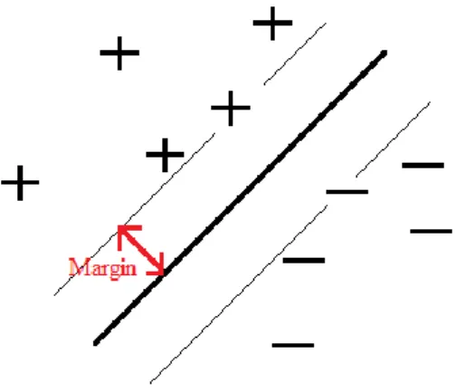
The aim of SVM is to maximize the margin between each class so that a good generalization performance on unseen test instances can be obtained. Although the subject was introduced in the late seventies (Vapnik, 1979), it has been receiving increasing attention, and so the time appears suitable for an introductory review. In Figure 2.2, there is a classification problem for two class (+, -) dataset. The aim is to find a hyperplane so that "+" data points take place in one side and "-" ones are placed in the opposite side of this separator. SVM uses a flexible representation of the class boundaries. For each side, the data points which are located on the boundaries where the hyperplane is maximally distant from them are called support
vectors and the gap between hyperplane and a support vector is known as margin.
Campbell and Ying (2011) states SVM generalization error, i.e. the upper bound as "the bound is minimized by maximizing the margin (
, where w is a normal
vector to bounding planes) i.e., the minimal distance between the hyperplane separating the two classes and the closest data points to the hyperplane" (Chapter 1, p. 2).
Figure 2.2 : Two class data points linearly separable by a hyperplane. According to the Figure 2.2, a linear support vector machine is illustrated and the hyperplane is constructed using a simple formulation w . x + b = 0 where "." denotes inner product, b is bias from the origin in the input space, w is weight determining the orientation and x are data points taking place in the hyperplane or normal to it. "+" data points are placed in terms of the formula w . x + b ≥ 0 while "-" instances are placed by applying w . x + b < 0 so that separation makes the classification process an easy task.
14
Even though SVM was originally developed for binary classification, it is now applied in both binary and multi-class data classification problems providing an acceptable prediction ability.
2.2.1 Non-separable case
Majority of the problems are not as simple as the given scenario in Figure 2.2 because data points cannot be convenient to be separated by a linear hyperplane due to non-linear clusterings found in data. For those cases, we enhance kernel functions to transform the non-linear data into a feature space so that linear classification can be applied. The choice of a kernel depends on the problem at hand because it depends on what we are trying to model. In the literature, there are many popular kinds of kernels defined to apply in complex machine learning problems such as polynomial kernel for modeling feature conjunctions up to the order of the polynomial and radial basis function kernel where circles (or hyperspheres) are picked out.
Lee, Yeh and Pao (2012) introduce SVMs for this kind of problems by making use of support vectors in discriminating between complex data patterns by generating a highly nonlinear separating hyperplane, that is implicitly defined by a nonlinear kernel map.
For training data xi ϵ Rn , i = {1, ..., m} with class labels y ϵ Rl such that yi = {-1, 1}
C-SVC can be formulated as an optimization problem given in equation 2.8.
s.t.
(2.8)
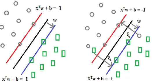
where w is the normal vector to the bounding planes (xTw + b = -1 for class "-" and xTw + b = 1 for class "+" according to Figure 2.3), b shows their position relative to the origin. is a slack variable for soft margins which is defined for linearly non-separable cases ( wTxi + b + ≥ +1 for class "+" and wTxi + b + ≤ -1 for class "+")
and 1-norm of , is called the penalty term. Due to the higher complexity of the separating hyperplane overfitting situation can occur by leading to poor generalization. In this direction, C>0 is used as a regularization parameter balancing the weights of the penalty term versus the margin maximization term .
15
Figure 2.3 : An example of linearly separable (left) and non-separable (right) SVM
LibSVM (Chang and Chih-Jen, 2011) is a C/C++ based package for easily implementing support vector machines in other languages/softwares such as Matlab, Python, Java and Octave. In order to deal with binary class and multi class problems, the library provides SVC type of SVM. Except from SVC, SVR (Support vector regression) is available for regression problems and one-class SVM is also present in the package. In this study, one of the SVM types, C-SVC is used to classify both binary and multi-class datasets.
For binary classification in C-Support Vector Classification, a solution is found to the following primal optimization problem:
s.t.
(2.9)
where is a function which maps data point xi into a higher dimensional space,
and C, b, w and parameters are same as the previous ones. Because of the probable high dimensionality of the vector w, it can be formulized by a dual problem:
s.t. , i = 1, ..., m
16
where e is a vector which is full of ones, Q represents a m by m positive semidefinite matrix, and Qij ≡ yiyjK(xi,xj) where K(xi,xj) is the kernel function as K(xi,xj) ≡
Once the problem is solved, then the optimal w satisfies
(2.11)
and the decision function is
(2.12)
In this study, radial basis function is selected as the kernel function for two samples x and x'. It is defined as in equation 2.13:
(2.13)
where we can define a parameter
α and result in
2.3 Ensemble Learning
Ensemble learning is a paradigm where multiple learners are trained to solve a machine learning problem and a final decision is made after combining each output of single learners according to some criteria. As No Free Lunch theorem states that there is no single model that works best for every problem the aim of the ensemble learning is to boost the accuracy of the single classifiers. Besides due to the possible noise in the data, overlapping data distributions and outliers generally single classifiers cannot achieve a certain classification accuracy. These have grown the needs to create ensemble techniques.
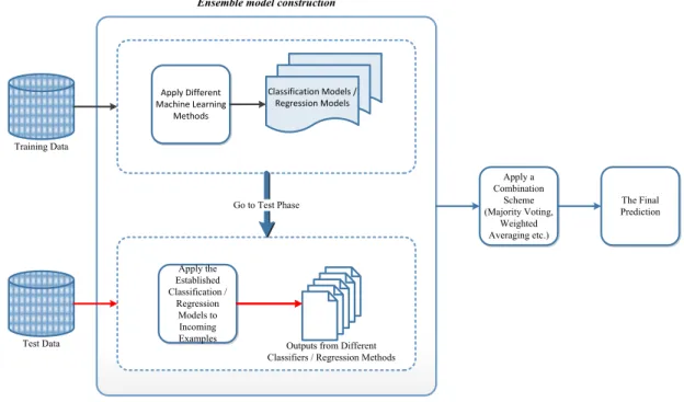
Establishing an ensemble model is made up of two stages. In the first part, a couple of base classifiers are generated in a parallel or sequential manner. Generally, in the sequential manner the construction of a base classifier may affect the construction of the subsequent classifiers. In the latter part, the resulting classifier outputs are combined to take a decision about the final classification of a new test instance. At this stage some type of combination schemes are applied such as majority voting for a classification problem. In the majority voting the class label is selected from the
17
majority of the individual classifiers’ class labels. In regression weighted averaging of the base regressors’ outputs gives the final prediction result. The basic framework of the ensemble modeling is depicted in Figure 2.4.
Training Data
Test Data
Ensemble model construction
Apply a Combination Scheme (Majority Voting, Weighted Averaging etc.) The Final Prediction Apply Different Machine Learning Methods Classification Models / Regression Models
Outputs from Different Classifiers / Regression Methods Apply the Established Classification / Regression Models to Incoming Examples Go to Test Phase
Figure 2.4 : Ensemble learning framework.
Model ensembles are among the highly effective techniques in machine learning and pattern recognition applications that generally outperforms other methods. Ensemble learning has already been applied in a variety of domains related to machine learning problems such as text categorization (Dong and Han, 2004), optical character recognition (Chellapilla et al, 2006), face recognition (Lu et al, 2006) and gene expression analysis (Tan and Gilbert, 2006) etc for searching a hypothesis space to reach the most accurate hypothesis by reducing the total error.
It is mostly preferred to classical single learning models because of three significant reasons. The first one is that there may be insufficient information in order to decide on which classifier performs better on the training data. A solution to this problem is therefore combining the ones which results in sufficiently well and it is a reasonable choice to apply. Another rationale is that the applied learning algorithm might practise imperfect search processes which ends up with sub-optimal hypotheses even if there exists a unique best hypothesis. The last reason is the case where ensemble strategy leads to a good approximation as one learner cannot reach a true target
18
function in the searching phase. On the other hand, choosing ensemble models comes at the cost of raised algorithmic and model complexity. Ensemble strategies can be obtained on either feature space, instance space or classifiers’ parameter space. Next we will detail one of the most successful ensemble learning on feature space namely random subspace methods.
2.3.1 Random subspace ensemble learning
Searching for a feature base that leads to a considerable classification performance is another challenging task to cope with. Even if there is a single input representation, by selecting random subsets from it we can train different classifiers on selected subspace of features, which is called the random subspace method (Ho, 1998).
Random Subspace Ensemble Learning "RS", also known as Attribute Bagging, is one of the most commonly used ensemble learning methods which plays an important role in finding the subset of informative features to correctly classify given signals. It is a wrapper method that can be used with any learning algorithm. The method is applied by classifying test instances with a chosen classifier along with randomly selected subsets of all possible features iteratively and with replacement. The feature base is changed in each iteration with the same number of randomly permuted features. If we name the whole constructed feature subspace as Xrs, and the
selected feature subspace at ithiteration as Xrs_i, K number of subspaces are created at
the end of the process in K iterative ensemble learning steps where Xrs = {Xrs_1, ...,
Xrs_K}. Table 2.1 shows the pseudo code of the random subspace ensemble learning
method.
Table 2.1 : The pseudo code of random subspace ensemble learning. Algorithm: Random subspace ensemble learning method
Input: training set X, number of features in the subspace s, number
of ensemble predictors K, predictor h
Output: ensemble model h = {h1, ..., hK} combination of whose
outputs is used to predict new test instances' class labels/regression results
For i = 1:K
Create a subspace sample data Xrs_i with s features selected at
random with replacement from X Apply the predictor hi to Xrs_i
End For
19
Note that by applying random feature subspaces, different predictors will deal with the same problem from different standpoints by resulting in more robust representation and diminishing the curse of dimensionality arising from high dimensional inputs.
2.3.2 Bagging
Bagging short for "bootstrap aggregating" is an ensemble learning approach which generates multiple exemplars of a predictor to lead to an aggregated learner by taking the combination of their outputs using a fixed rule. It provides a way to present variability between the different models within a committee. Creation of the multiple exemplars is done via making bootstrap replicates of the learning set.
Logic behind the bootstrap creation is treated as follows. Assume that we have a dataset X = {x1, ..., xm} with m data points. If we generate a new dataset XBagged
whose instances are randomly drawn from the original dataset as the same number of instances with replacement, it is the case where some number of data points are repeated containing duplicates in XBagged and some others in the original dataset are
not included now. A particular instance which is chosen for a bootstrap sample of size mcan be calculatedas follows:
(2.14)
which is about two-third and has limit 1-1/e = 0.632 for m→∞(Flach, 2012, Chapter 11). This means that each bootstrap sample is likely to leave out about a third of the data points. This difference between bootstrap models is exactly what we want to give rise to diversity among the models in the ensemble. An iterative process is performed by repeating this procedure K times and resulting in K randomly generated datasets. Table 2.2 displays the pseudo code of the general framework of bagging algorithm.
2.4 Active Learning
In passive learning, a bunch of training examples and their class labels are provided to the learning algorithm. In many machine learning problems, we need to cope with significant number of unlabelled examples whose labeling is mostly time-consuming and expensive to obtain. Active learning is a framework where abundant unlabeled data and few labeled samples are available.
20
Table 2.2 : The pseudo code of bagging. Algorithm: Bagging
Input: training set X, number of instances m, number of ensemble
predictors K, predictor h
Output: ensemble models h = {h1, ..., hK} combination of whose
outputs is used to predict new test instances' class labels/regression results
For i = 1:K
Create a bootstrap sample data Xbagging_i with selecting n data
points randomly with replacement from X Apply the predictor hi to Xbagging_i
End For
Return h = {h1, ..., hK} ensemble model
The framework resolves the labeling problem by asking the labels of some intelligently selected examples to a trained expert or an oracle. The selected data points are usually the optimal ones which boost the number of correctly classified instances upon they are labeled and incorporated into the training phase.
Active learning scenario has been applied in various machine learning real-world applications such as image classification and retrieval (Zhang and Chen, 2002), text classification (Tong and Koller, 2001), email filtering, web searching, video classification and retrieval, information extraction and speech recognition etc.
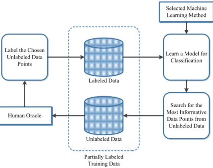
The fundamental purpose of active learning is to improve the accuracy of the initial classifier by adding new training examples from unlabelled dataset which are selected using a selection criterion i.e. informativeness measure. The learner may start the classification task with few number of labelled training data, then in each iteration one or more unlabeled instances are carefully chosen to be added to the training examples after its class label is determined by an oracle. This process is implemented iteratively by the selection of the most informative unlabeled data points which will help improve the prediction ability. Figure 2.5 points out the generalized active learning framework.
In the matter of applying active learner, sources of unlabelled instances play an important role. In literature, there are three main categories of sources of unlabelled data (Roederer, 2012; Settles, 2010):
21 Unlabeled Data
Labeled Data
Partially Labeled Training Data
Learn a Model for Classification Selected Machine Learning Method
Search for the Most Informative Data Points from Unlabeled Data Human Oracle
Label the Chosen Unlabeled Data
Points
Figure 2.5 : Active learning framework.
query synthesis in which the learner asks the labels of unlabelled data points
from some underlying distribution also including the queries that the learner produces de novo without the need for a distribution.
stream-based sampling where unlabelled instances are handled one by one
through sampling from an actual distribution to decide whether they should be integrated into the set of labelled instances or not. It is suitable for special situation where the memory and storage capacity is limited.
pool-based sampling which is the mostly applied sampling scenario that the
learner chooses instances from a pool of unlabelled data to query by using a greedy approach through examining informativeness of each.
In pool-based sampling, a significant question arises in the case of how to select and assess the most informative data point among the unlabeled examples. Perhaps the simplest way is to query instances where the learner is least certain and this process is known as uncertainty sampling. One of the most popular uncertainty sampling techniques is based on entropy. We want to choose the examples which leads to the greatest reduction in entropy upon its class label is known. Calculating the entropy over the distribution of possible class labels results in a value that represents the amount of information needed. "The more entropy in the distribution, the more uncertain the choice of class label for that data value, and the more informative that
22
query would be" (Roederer, 2012). A generalized entropy-based query sampling strategy can be defined as in equation 2.15:
where i = {1, ..., c}
(2.15) where x refers to any instance, y is the class of the instance x, c is the number of classes and θ is the parameters in the classifier model h.
According to Holub et al. (2008), "Active learning adaptively prioritizes the order in which the training examples are acquired which can significantly reduce the overall number of training examples required to reach near-optimal performance" (p. 1).
23 3. THE PROPOSED METHOD
In this study, one of the supervised classification algorithms, dictionary learning, is applied in combination with active learning framework using the strength of ensemble classifier strategies. In the first step, Bagging and Random Subspace ensemble methods are performed by using dictionary learning as the base classifier and in the latter part, Active Learning is applied by showing the effect of using the most informative unlabeled instances while modeling dictionary base.
3.1 Dictionary Ensembles Using Random Subspaces and Bagging
Bagging and Random Subspace methods are the most commonly used ensemble learning methods which play an important role in finding the subset of instances and features to obtain diverse classifiers given data samples. Following the idea behind dictionary learning, ensemble learning methods can be merged into the process to boost the correctly classified number of instances. Accordingly, in this study dictionary learning is used as a base classifier with Random Subspace and Bagging methods. Random Subspace Dictionary Learning (RDL) and Bagging Dictionary Learning (BDL) algorithms creates K dictionaries for each class in the training set using randomly selected features for RDL and instances for BDL. Class label for a test instance is determined by picking up the majority class label among the results of all K dictionaries. The pseudo-code of the algorithms is given in Table 3.1.
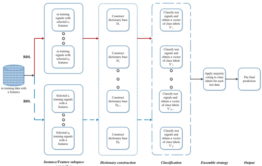
The framework of the proposed dictionary learning algorithms is shown in Figure 3.1. Initially, according to the choice of ensemble learning strategies, either BDL or RDL, s instance/feature subspaces are generated. In the dictionary construction phase, each subspace produces a dictionary base. Test data are classified using the ensemble dictionary learning classifiers after dictionary construction phase. As a result, ensemble strategy produces a final prediction by applying majority voting on class labels obtained in each instance/feature subspace.
24
Table 3.1 : The pseudocode of the proposed ensemble methods. Algorithm: Ensemble dictionary learning
Input: training set X ϵ Rmxn, training class labels Y ϵ Rm, number of features n,
number of selected feature/instances s, number of ensemble dictionaries K, number of classes c, test set X' ϵ Rwxn, number of training instances m, number of test instances w
Output: predicted class labels Y' for test instances
Training: For i = 1:K
switch(ensemble_algorithm) case RDL:
Select s random features from X
Create Xr ϵ Rmxs using selected features
case BDL:
Select s random instances from X Create Xr ϵ Rsxn using selected instances
For each class in the training set Xr: Train dictionaries {D1, D2, ..., Dc}
Di = {D1, D2, ..., Dc}
End For
Testing: Input a test instance vector x' from test set X' For i = 1:K
Calculate using (2.7) and Di End For
Classify x' using majority voting on 's
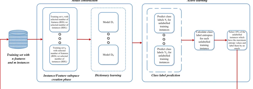
3.2 Active Learning Based Data Classification Using Dictionary Ensembles The proposed active learning scenario is applied in combination with Random Subspace Dictionary Learning and Bagging Dictionary Learning methods as the base classifiers. Initially, 20% of the whole dataset is used as training data to construct a supervised dictionary model.
To form each random subspace ensemble, feature subspace is iteratively reduced by randomly chosen attributes with replacement. Using the dictionary model, unlabeled instances are classified into appropriate classes. At each iteration in order to select the instances to be queried, entropy query strategy is employed by computing the class label entropies using equation 2.15. Unlabeled instances are sorted in a descending order based on their entropies. At each iteration, the data samples that have the highest entropy values are asked to the oracle and 10% of the unlabelled instances are added to the training data. Figure 3.2 displays the scenario schematically.
25
Performing active learning ensures choosing the most informative instances to training set, by doing so, atoms can be updated or new atoms can be added to the dictionaries which may improve the sparse representations of the instances.
26 m training signals with selected s1 features m training signals with selected sK features Apply majority voting to class labels for each
test data RDL
m training data with n features The final prediction Selected s1 training signals with n features Selected sK training signals with n features BDL Instance/Feature subspace generation Co