Wayne State University Dissertations
1-1-2017
Reliability Based Design Optimization Of Load
And Rating Models For Bridge Structures In
Michigan
Vahid Kamjoo
Wayne State University,Follow this and additional works at:https://digitalcommons.wayne.edu/oa_dissertations
Part of theCivil Engineering Commons
This Open Access Dissertation is brought to you for free and open access by DigitalCommons@WayneState. It has been accepted for inclusion in Wayne State University Dissertations by an authorized administrator of DigitalCommons@WayneState.
Recommended Citation
Kamjoo, Vahid, "Reliability Based Design Optimization Of Load And Rating Models For Bridge Structures In Michigan" (2017).
Wayne State University Dissertations. 1819.
© COPYRIGHT BY VAHID KAMJOO
2017
ii
DEDICATION
iii
ACKNOWLEDGMENTS
I take immense pleasure in thanking Dr. Christopher D. Eamon, Associate Professor at the Department of Civil and Environmental Engineering at Wayne State University, for his guidance, support and professional academic supervision, which assisted me in completing this
Ph.D. dissertation.
I am grateful to Dr. Christopher D. Eamon, Dr. Hwai-Chung Wu, Dr. Mumtaz Usmen, from the Department of Civil and Environmental Engineering at Wayne State University, and Dr. Kazuhiko Shinki, from the Department of Mathematics at the Wayne State University, for
iv
PREFACE
DEVELOPING RELIABILITY BASED DESIGN OPTIMIZATION TO CALCULATE LOAD FACTOR
The main research objectives of this study are to determine the most accurate and consistent method for predicting live load factor for design and rating of MDOT bridge, determine the reliability index of load factor for different bridge types, develop Reliability Based Design Optimization to calculate the optimized load factor.
v
TABLE OF CONTENTS
DEDICATION ... ii
ACKNOWLEDGMENTS ... iii
PREFACE ... iv
LIST OF TABLES ... viii
LIST OF FIGURES ... x
CHAPTER 1: INTRODUCTION ... 1
1.1 Statement of the Problem ... 1
1.2 Background ... 2
1.3 Objective and Scope ... 6
CHAPTER 2: LITERATURE REVIEW ... 7
2.1 MDOT Reports and Standards ... 9
2.2 Current MDOT Practice ... 10
2.3 NCHRP Reports ... 12
2.4 Multiple Presence Modeling ... 17
2.5 Collecting and Analyzing WIM Data ... 21
2.6 Development of Time-Adjusted Load Effect Statistics ... 23
2.7 Load Model Development for Bridge Design and Evaluation ... 25
2.8 Reliability Analysis Methods ... 29
2.9 Reliability Based Design Optimization ... 31
CHAPTER 3: ANALYSIS OF WIM DATA... 34
3.1 WIM SITES ... 34
vi
3.2.1 Filtering Criteria... 37
3.2.2 Comparison to Permit Data ... 39
3.2.3 Legal and Non-Legal Vehicles ... 41
3.2.4 Data Quality Checks ... 41
CHAPTER 4: MULTIPLE PRESENCE FREQUENCIES ... 44
4.1 General side by side probabilities ... 44
4.2 Side by side probability of special permit vehicles ... 45
4.3 Effect of Traffic Direction ... 46
CHAPTER 5: VEHICLE LOAD EFFECTS ... 47
5.1 Load Effects from WIM Data ... 47
CHAPTER 6: RELIABILITY MODELS ... 48
6.1 Reliability Based Design procedure ... 48
6.1.1 One Lane Effects... 48
6.1.2 Two Lane Effect ... 50
6.1.3 For Both 1 and 2-Lane Effects ... 51
6.2 Reliability Based Rating procedure ... 56
6.2.1 One Lane Effects... 57
6.2.2 Two Lane Effect ... 57
6.2.3 For Both 1 and 2-Lane Effects ... 58
6.3 Bridge Structures Considered ... 60
6.4 Data Projection ... 61
CHAPTER 7: RELIABILITY Based Design Optimization ... 68
vii
7.2 Design Variables ... 71
7.3 Load Effects Calcilation ... 72
7.4 Reliability Analysis ... 72
7.5 Objective Function ... 74
7.5.1 Optimize Beta Value When LF is Constant ... 74
7.6 Constraint ... 75
7.7 Results ... 75
7.7.1 Design ... 76
7.7.2 Rating ... 86
CHAPTER 8: SUMMARY, CONCLUSIONS AND RECOMMENDATIONS ... 92
8.1 Summary ... 92
8.2 Recommendations ... 93
APPENDIX A: STATEWIDE MDOT WIM SENSOR LOCATIONS ... 98
APPENDIX B: SUMMARY OF WIM DATA ... 102
APPENDIX C: VEHICLE LOAD EFFECTS ... 174
APPENDIX D: BRIDGE STRUCTURE DEAD LOADS ... 191
REFERENCES ... 194
ABSTRACT ... 205
viii
LIST OF TABLES
Table 3.1. WIM Stations Used for Reliability calibration ... 35
Table 3.2. Small Vehicles Filtering Criteria ... 37
Table 3.3. WIM Data Filtering Criteria ... 38
Table 6.1. Statistical Parameters for DF ... 53
Table 6.2. Random Variable Statistics ... 54
Table 7.1. Design variables ... 71
Table 7.2. Constraints ... 75
Table 7.3. Beta statistics(Steel bridge, Design, Moment and Shear) ... 77
Table 7.4. Beta statistics(Steel bridge, Design, Moment and Shear) ... 79
Table 7.5. Beta statistics(Steel bridge, Design, Moment)... 80
Table 7.6. Beta statistics(Steel bridge, Design, Shear) ... 82
Table 7.7. Beta statistics(Steel bridge, Design, Shear) ... 83
Table 7.8. Beta statistics(PC, Design, Moment) ... 85
Table 7.9. Beta statistics(PC, Design, Shear) ... 86
Table 7.10. Governing trucks through the 28 Michigan legal trucks ... 86
ix
Table 7.12. Beta statistics(Steel bridge, Rating, Shear) ... 89
Table 7.13. Beta statistics(PC, Rating, Moment) ... 90
Table 7.14. Beta statistics(PC, Rating, Shear) ... 91
x
LIST OF FIGURES
Figure 3.1. WIM Sites With ADTT ≥5000 ... 35
Figure 3.2. WIM Sites With ADTT ~2500 ... 36
Figure 3.3. WIM Sites With ADTT ~1000 ... 36
Figure 3.4. WIM Sites With ADTT ~400 ... 37
Figure 6.1. CDF of Top 5% of All Vehicles, Single Lane Simple Span Moments ... 64
Figure 6.2. Normal Fit to 75 Year Projection, Singe Lane, Normal Probability Plot ... 65
Figure 6.3. CDF of Top 5% of All Vehicles, Two Lane, Normal Probability Plot ... 65
Figure 6.4. Normal Fit to 75 Year Projection, Two Lane, Normal Probability Plot ... 66
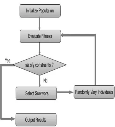
Figure 7.1. Genetic Algorithm flow chart ... 70
Figure 7.2. Comparison of 6-axle truck, HL93 and HL93mod for all spans ... 76
Figure 7.3. 6-axle truck configurations ... 77
Figure 7.4. Comparison of 6-axle truck, HL93 and two 4-axle trucks ... 78
Figure 7.5. 4-axle truck configuration for spans < 65 ft ... 78
Figure 7.6 4-axle truck configuration for spans > 65 ft ... 78
Figure 7.7 Comparison of 5-axle truck, HL93 and HL93mod for all spans ... 79
xi
Figure 7.9. Comparison of 5-axle truck, HL93 and two 3-axle trucks ... 81
Figure 7.10. 3-axle truck configuration for spans > 65 ft. (D1)... 81
Figure 7.11. 3-axle truck configuration for spans < 65 ft. (D2)... 81
Figure 7.12. Comparison of 6-axle truck, HL93 and two 4-axle trucks ... 82
Figure 7.13 4-axle truck configuration for spans > 65 ft. (D3)... 83
Figure 7.14 4-axle truck configuration for spans < 65 ft. (D4)... 83
Figure 7.15 Comparison of 10-axle truck, HL93 and two 3-axle trucks ... 84
Figure 7.16. 3-axle truck configuration for spans > 65 ft. (D5)... 84
Figure 7.17. 3-axle truck configuration for spans < 65 ft. (D6)... 84
Figure 7.18. Comparison of 6-axle truck, HL93 and HL93mod ... 85
Figure 7.19. 6-axle truck configuration for all spans (D7) ... 86
Figure 7.20 Comparison of 4-axle truck and Michigan govern trucks ... 87
Figure 7.21 4-axle truck configuration for all spans (R1) ... 87
Figure 7.22 Comparison of 4-axle truck and Michigan govern trucks ... 88
Figure 7.23. 10-axle truck configuration for all spans (R2) ... 88
Figure 7.24. Comparison of 3-axle truck and Michigan govern trucks ... 89
xii
Figure 7.26. Comparison of 4-axle truck and Michigan govern trucks ... 90 Figure 7.27. 6-axle truck configuration for all spans (R4) ... 91
CHAPTER 1: INTRODUCTION
1.1 Statement of The Problem
The load models developed for Load and Resistance Factor Design (LRFD) (AASHTO LRFD 2010) and Load and Resistance Factor Rating (LRFR) (AASHTO MBE 2011) are based on a generic, small sample of truck traffic. Although some adjustments are specified for average daily truck traffic (ADTT), these models are otherwise assumed to apply to all bridges. However, these data were used to determine bridge design loads to be used across all states. This is problematic as many states have vehicular traffic loads that differ significantly from those used to develop the AASHTO LRFD live load. An example of one such state is Michigan. Although the Michigan Department of Transportation (MDOT) has modified both the design as well as the rating process to better correspond to Michigan loads (Curtis and Till 2008), these modifications are similarly based on a generic and greatly limited data set. Of particular concern is heavy vehicle side-by-side frequency, which was taken as a constant value across structures for development of design loads (1/15 for the LRFD code). For development of LRFR evaluation and rating loads, side-by-side heavy truck probability was taken as 1/15 for an ADTT (Average Daily Truck Traffic) of 5000 (1/30 for the modified rating loads used by MDOT); as 1/100 for an ADTT of 1000, and as 1/1000 for an ADTT of 100 (Moses 2001). The assumptions used for heavy truck side-by-side frequency has a significant effect on the expected load on bridge girders. Applying this generic load model to Michigan bridges, which may have significantly different traffic profiles than those used to develop the LRFD/LRFR load models, may result in inconsistencies in safety level for design as well as evaluation. Moreover, as the LRFD/LRFR side-by-side multiple presence assumptions are generally thought to be overly-conservative (Curtis and Till 2008; Moses 2001; Ghosn 2008), use of the resulting design and evaluation loads leads to some Michigan bridges being over-designed
as well as under-rated, potentially wasting design and construction resources and unnecessarily restricting truck traffic.
1.2 Background
In 1994, the 1st Edition of the AASHTO LRFD Bridge Design Specifications was published, with the intent to provide a consistent level of reliability to bridge structures by using the probabilistically calibrated LRFD format. Later, the Manual for Bridge Evaluation (MBE) was published by AASHTO in 2008, replacing the 1998 Manual for Condition Evaluation of Bridges (based on Load Factor Rating, LFR) and the 2003 Manual for Condition Evaluation and Load and Resistance Factor Rating (LRFR) of Highway Bridges. In 2007, FHWA required that bridge structures be designed with LRFD as opposed to the Load Factor Design (LFD) approach previously used by MDOT. Moreover, in 2010, FHWA required that structures designed by LRFD were to be rated with LRFR, as in the MBE. The result of moving to LRFD/LRFR from LFD/LFR was significant for MDOT. Most bridges previously designed by LFD and rated by LFR could carry all Michigan legal loads and Class A permit overloads. However, if structures were designed and rated according to the unmodified LRFD and LRFR approaches, many bridges would be unable to carry some Michigan legal loads as well as permit overloads (Curtis and Till 2008).
The differences between using LRFD/LRFR and LFD/LFR are primarily a result of the revised LRFD/LRFR load models. Due to the limited amount of traffic data available at the time, the LRFD load model was developed from a 2-week sample of truck weights measured in Ontario in 1975. Moreover, several assumptions were made to allow for data extrapolation to the 75-year expected mean maximum load used to calibrate the design load. Of particular importance is the presence of side-by-side trucks in adjacent lanes, which has significant impact on load effects. For the LRFD calibration, it was assumed that every 1/15 ‘heavy’ truck was side-by-side with another,
where a ‘heavy’ truck was taken as the top 20% of the truck population. Moreover, it was assumed that 1/30 side-by-side truck events occur with fully correlated (i.e. identical) truck weights. These assumptions resulted in a model which stipulated that, for every 3rd random truck passage, it is side-by-side with another truck, and for every 1/450 heavy truck crossing, it is side-by-side with an equally heavy truck. Simulations from this model determined that the case of two side-by-side, fully-correlated trucks governed the maximum load effect. In this case, each truck was 85% of the maximum 75-year single lane truck, which were equivalent to 1.0-1.2 times the equivalent HL-93 load, depending on bridge span. This maximum governing load was assumed normally distributed with coefficient of variation from 0.14 to 0.18, depending on span length. This model led to the development of the HL-93 load with live load factor of 1.75 (without impact) and associated multi-lane and ADTT adjustment factors, to meet the minimum target reliability level for LRFD design of β=3.5. Note that bridges with spans greater than 200 ft were not considered (Nowak 1999).
For bridge evaluation with LRFR, for ADTT ≥ 5000, the LRFD truck traffic model with side-by-side probability of 1/15 for heavy trucks was maintained for consistency, although this was known to be an extremely conservative value (Moses 2001; Ghosn 2008; Sivakumar 2007). For the 2 and 5-year return periods originally used to develop the LRFR load models, use of the LRFD traffic load assumptions resulted in a mean maximum load event to be the multiple presence of two side-by-side 120 kip (for a 2-year return period) or 130 kip (for a 5-year return period) trucks, of 3S2 equivalent truck configurations. This governing live load was assumed to be lognormally distributed with a coefficient of variation of 0.18. To maintain the target evaluation reliability levels of β=3.5 for inventory ratings and β=2.5 for operating ratings using LRFR with this model, the resulting legal load factor was 1.8 for truck weights up to 100 kips (for ADTT ≥
5000). To maintain the target reliability for permit trucks, the live load factor was linearly interpolated between 1.8 and 1.3 for truck gross vehicle weights (GVWs) between 100 and 15.
The conservativeness of multiple presence assumptions in LRFD/LRFR can be practically seen in the work of Ghosn, who studied Weigh-in-Motion (WIM) data from multiple states and generally found that the reliability levels associated with two-lane load effects, as designed/rated, are significantly higher than the one-lane load effects. In California, for example, the LRFD load factor would require a reduction from 1.75 to 1.2 for the two-lanes loaded case to maintain a consistent reliability level with the one-lane loaded case (Ghosn 2008).
A previous study considering Michigan traffic loads (Eamon et. Al. 2014) found that there is a significant variation in the required live load factor from one bridge to another to produce uniform levels of reliability. As the pattern of required load factors is relatively complex, an ideal approach to minimize the load factor variation for all bridge designs is the use of an optimization procedure. There are various optimization techniques that can be used to solve engineering problems, such as classical methods and heuristics. Some of classical methods include sequential quadratic programming (SQP) and calculus-based gradient techniques. SQP is an iterative method that can be used to solve a nonlinear optimization problem. This method is used in problems for which the objective function and constraints are continuously differentiable (Soler et. al. 2013). Calculus-based gradient techniques require the construction or approximation of derivative information. This method can only hope to find local optima (Goldberg and Kuo, 1987). Some heuristics methods include particle swarm optimization (PSO) (Kennedy 2011) and artificial bee colony optimization (Karaboga and Basturk 2007).
In design optimization, stochastic uncertainty associated with load intensity, material properties, geometric dimensions, etc. is represented by random variables and propagated by
mathematical models that quantify variability in responses that depend on such random variables. Probability theory is most commonly used to model stochastic uncertainty in design optimization. This combination of probabilistic modeling and mathematical design optimization framework leads to reliability-based design optimization (RBDO). There are multiple ways of formulating and solving an RBDO problem (Enevoldsen and Sorensen 1994; Frangopol 1995; Tu et al. 1999; Rais-Rohani and Xie 2005; Kharmanda and Olhoff 2007; Aoues and Chanteaueuf 2010, etc). Different approaches for the evaluation of probabilistic constraints have been developed (Enevoldsen and Sorensen 1994; Tu et al. 1999). More recently, Du and Chen (2004) proposed the replacement of each probabilistic constraint with an equivalent deterministic constraint and the decoupling of reliability analysis and design optimization in each design cycle, whereas Qu and Haftka (2004) suggested the use of a probability safety factor in the modeling of each probabilistic constraint.
Previous research has applied design optimization on specific structures, such as to minimize weight or maximize performance criteria such as strength or stiffness. The propose of this study is to use design optimization to in a new way: to develop an optimal load model that can be used to design and load rate a variety of different bridge structures. This would allow any structure that uses the developed model to be optimally designed or rated, without the need for applying further, computationally intensive optimization techniques to each structure individually. The goal of the optimization is to determine an idealized live load (truck model) that produces the lowest discrepancies in reliability among the different bridge structures, while under the constraints that no bridge designed or rated using the model falls below the minimum required reliability level.
1.3 Objective and Scope
The goal of this study is to develop and optimal live load model (in the form of idealized trucks) that can be used for both design and rating. The specific research objectives are to:
• Clean, sort, and analyze a large quantity of weight in motion (WIM) truck traffic data collected from Michigan roadways.
• From a detailed analysis of the WIM data, statistically quantify the load effects, in terms of moments and shears, generated by the recorded truck traffic, extrapolated to the appropriate return periods for design and evaluation (rating).
Based on the load effect statistics, develop corresponding probabilistic load models and incorporate these models into a reliability model for bridges.
• Develop a procedure to apply reliability based design optimization (RBDO) to develop design and rating load models in order to minimize variation in bridge reliability.
• Propose recommendations for vehicular live loads to be used for bridge design and evaluation, such that bridges can meet uniform target reliability levels and avoid unnecessary traffic restrictions.
CHAPTER 2: LITERATUR REVIEW
For bridge design using the AASHTO LRFD Bridge Design Specifications (2010), due to the limited amount of traffic data available at the time, the LRFD load model was developed from a 2-week sample of truck weights measured in Ontario in 1975. Moreover, several assumptions were made to allow extrapolation of the data to the 75-year expected mean maximum load used to calibrate the design load. For multiple presence of side-by-side trucks in adjacent lanes, it was assumed that every 1/15 ‘heavy’ truck was side-by-side with another, where a ‘heavy’ truck was taken as the top 20% of the truck population. It was also assumed that 1/30 side-by-side truck events occur with fully correlated (i.e. identical) truck weights. These assumptions resulted in a model which stipulated that, for every 3rd. random truck passage, it is side-by-side with another truck, and for every 1/450 heavy truck crossings, it is side-by-side with an equally heavy truck. Simulations from this model determined that the case of two side-by-side, fully-correlated trucks governed maximum load effect. The governing trucks were each 85% of the maximum 75-year single lane truck, which were equivalent to 1.0-1.2 times the equivalent HL-93 load, depending on bridge span. This maximum governing load was assumed normally distributed with coefficient of variation from 0.14 to 0.18, depending on span length. In addition to vehicular live load, the statistics for other random variables (RVs) necessary for reliability assessment were established for the AASHTO LRFD Code development. These include bridge component dead loads and girder moment and shear resistances. These RVs, as well as the corresponding reliability models and associated limit states have been identified and quantified for steel, concrete, and prestressed concrete bridge girders in NCHRP 368 (Nowak 1999), as used for the calibration of the LRFD code. Using these statistics for reliability assessment led to the development of the HL-93 load with live load factor of 1.75 (without impact) and associated multi-lane and ADTT adjustment
factors, to meet the minimum target reliability level for LRFD design of β=3.5. Bridges with spans greater than 200 ft were not considered.
The Manual for Bridge Evaluation (MBE) was published by AASHTO in 2008, replacing the 1998 Manual for Condition Evaluation of Bridges (based on Load Factor Rating, LFR) and the 2003 Manual for Condition Evaluation and Load and Resistance Factor Rating (LRFR) of Highway Bridges. In the original publication of the MBE, for bridge evaluation with LRFR, for AADT ≥ 5000, the LRFD truck traffic model with side-by-side probability of 1/15 for heavy trucks was maintained for consistency, although this was known to be an extremely conservative value (Ghosn 2008; Sivakumar et al. 2007). It was also taken as 1/100 for an ADTT of 1000, and as 1/1000 for an ADTT of 100. For the 2 and 5-year return periods used to develop the LRFR load models, use of the LRFD traffic load assumptions resulted in a mean maximum load event to be the multiple presence of two side-by-side 120 kip (for a 2-year return period) or 130 kip (for a 5-year return period) trucks, of 3S2 equivalent truck configurations. This governing live load was assumed to be lognormally distributed with a coefficient of variation of 0.18. To maintain the target evaluation reliability levels of β=3.5 for inventory ratings and β=2.5 for operating ratings using LRFR with this model, the resulting legal load factor was 1.8 for truck weights up to 100 kips (for ADTT ≥ 5000). To maintain the target reliability for permit trucks, the live load factor was linearly interpolated between 1.8 and 1.3 for truck gross vehicle weights (GVW)s between 100 and 150 kips.
The MBE was later revised in 2011 (Sivakumar and Ghosn 2011) using WIM data from six states (New York, Mississippi, Indiana, Florida, California, and Texas). Four vehicle scenarios on a bridge were considered: a permit vehicle alone; two routine permit vehicles side-by-side; a routine permit vehicle alongside a random vehicle; and a special permit alongside a random
vehicle. Based on a 5-year return period, the revisions recalibrated the LRFR live load factors to result in a target reliability level of β=2.5 for permit loads, with a minimum level of β=1.5. Using the LRFR rating procedures, permit live load factors varied from 1.4 to 1.15 using two- lane load distribution factors, depending on ADTT and the load effect (gross vehicle weight divided by truck axle length).
2.1 MDOT REPORTS AND STANDARDS
MDOT released several research reports that involve load model development from WIM data, including RC-1413 (Van de Lindt and Fu 2002), which estimates the reliability of MDOT bridges using Michigan WIM data; RC-1466 (Fu and Van de Lindt 2006), which calibrated the live load factor for design using LRFD based on WIM data; and R-1511 (Curtis and Till 2008), which developed modified load and rating models for LRFD/LRFR based on NCHRP 454 (Moses 2001) and earlier reports.
From the information in these reports, best summarized in R-1511, MDOT determined that if structures were designed and rated according to the unmodified LRFD and LRFR approaches, many bridges would be unable to carry some Michigan legal loads as well as permit overloads (which were previously allowed under the Manual for Condition Evaluation of Bridges). Under the LFR approach, MDOT overload vehicles were assumed to have no multiple presence with other similar heavy trucks on a bridge, but using the LRFR system in the MBE, multiple presence is assumed, and this subject the overload vehicles to the multi-lane GDFs and load factors associated with legal-heavy vehicles, causing the lower bridge ratings under the LRFR approach.
As a result, MDOT modified both the design as well as the rating process to better correspond to Michigan loads, although these modifications are based on a generic and greatly limited data set. The modifications were designed to avoid the restrictive results of LRFD/LRFR
on Michigan traffic, and involved changing LRFR load factors for legal as well as overload vehicles, based on WIM data from Metro Detroit area bridges as well as other sources. This resulted in the LRFR- mod provisions, which present a series of adjusted load factors to be used for bridge evaluation. However, the LRFR-mod rating factors were based on limited, generic (although from Michigan) multiple presence data, where a multiple presence probability of 1/30 was used to develop the LRFR-mod load factor for AADT ≥ 5000. This adjustment did not completely solve the problem of new bridges being under-rated for traffic loads that were previously allowed, so MDOT additionally changed the base LRFD design load to the HL-93-mod load, which considers an additional single 60-kip axle load as well as an increased load factor of 1.2 over the LRFD loads. With these modifications in rating and design, the ratios of Michigan legal loads and overload moments to design moments were returned to values less than 1.0 for spans less than 200 ft. (longer spans were not investigated).
The MDOT Bridge Analysis Guide (2009) documents 28 common legal vehicle configurations, while the legal loads greater than 100 kips are classified as legal-heavy vehicles. For purposes of this report, routine permits as described as vehicles that exceed the legal loads but produce load effects (i.e. moment and shear) that fall below the requirements for a special permit; i.e. the lowest overload classification (C). Vehicles that exceed the Class C limit are special permit vehicles and may be issued a single passage permit over specific structures.
2.2 CURRENT MDOT PRACTICE
Based on some of this previous research, to avoid the restrictive results of LRFD/LRFR on Michigan traffic described above, MDOT modified the LRFR load factors for legal as well as overload vehicles, based on WIM data from Metro Detroit area bridges as well as other sources, resulting in the LRFR-mod provisions, which present a series of adjusted load factors to be used
for bridge evaluation. This did not completely solve the problem of new bridges being under-rated for traffic loads that were previously allowed, so MDOT additionally changed the base LRFD design load to the HL-93-mod load, which considers an additional single 60 kip axle load as well as an increased load factor of 1.2 over the LRFD loads. With these modifications in rating and design, the ratios of Michigan legal loads and overload moments to design moments were returned to values less than 1.0 for spans less than 200 ft (longer spans were not investigated) (Curtis and Till 2008).
As noted, a critical issue involving use of the LRFD and LRFR design and evaluation loads is the assumption used for multiple presence of side-by-side trucks, as this has a large impact on load effect. For example, under the LFR approach, MDOT overload vehicles were assumed to have no multiple presence with other similar heavy trucks on a bridge, but using the LRFR system in the Manual For Bridge Evaluation (MBE) (AASHTO 2011), multiple presence is assumed, and this subjects the overload vehicles to the multi-lane girder distribution factors (GDFs) and load factors associated with legal-heavy vehicles, causing the lower bridge ratings under the LRFR approach. Although this issue was accounted for in general by using the LRFR-mod rating load factors and HL-93-mod loads, the LRFR-mod rating factors were based on limited, generic (although from Michigan) multiple presence data. This recognition opens an opportunity to further refine the LRFR-mod as well as the HL-93-mod rating and design loads to more precisely account for multiple presence using the recently available, high-frequency time stamp WIM data for Michigan roadways. The use of this data provides a basis to recalibrate the design and rating methods and may result in a more uniform level of reliability across structures, more realistic criteria for posting restrictions and granting permits, as well as a more consistent expenditure of design and maintenance resources.
2.3 NCHRP REPORTS
NCHRP Report 368 (Nowak 1999) describes the development of the LRFD load model discussed above, while NCHRP Reports 454 (Moses 2001) and 20-07(285) (Sivakuman and Ghosn 2011) describe the development of the LRFR load models. In NCHRP 454, it was found that the characterizing multiple presence (multiple trucks crossing the bridge simultaneously) probability for load modeling is difficult, as multiple presence is affected by traffic volume, speed, road grade, weather, traffic obstacles, truck grouping, as well as other parameters. Moreover, load effects from multiple presence are strongly interlinked with truck headway distance (i.e. distance between trucks), which is also a function of various road and traffic conditions. The LRFR live load factor is given in NCHRP Report 454 (Moses 2001), as:
W WT L 72 240 8 . 1 (1.1)
Where W = gross weight of vehicle and WT = expected maximum total weight of rating and alongside vehicles, calculated as: WT + RT + AT. In the latter expression, RT = rating truck
and is computed for legal loads as: 3 2
*
S ADTT T
T W t
R or for permit load as:
along ADTT
T P t
R *
Here, W∗ = mean value of the top 20% of legal trucks taken from the
3S2 population; = standard deviation of the top 20% of legal trucks; P = weight of permit truck; and ∗ = standard deviation of the top 20% of the alongside trucks. The alongside truck,
, is compute as: AT W*along tADTT *along. In this equation, ∗ = mean of the top 20%
of alongside trucks.
In the above expressions, = fractile value corresponding to the number of side-by- side events, N. The number of side-by-side crossings is computed as:
) (% ) ( ) ( ) 365 ( ) ( )
( evaluation period P/ of record
year days ADTT legal N s s (1.2) ) ( ) ( ) 365 ( ) ( ) ( P evaluation period Ps/s year days N permit N (1.3) Where NP = number of observed single trip permits (STPs) in the WIM data extrapolated over the evaluation period and Ps/s = probability of side-by-side concurrence. LRFD and LRFR calibrations assumed a 1/15 (6.7%) probability of side-by-side events for truck passages. This assumption was based on visual observations and is conservative for most sites.
In an effort to refine load models for special hauling vehicles, NCHRP 575 (Sivakumar et al. 2007) developed a multiple presence model with additional complexity. Different multiple presence statistics were calculated for variations in bridge span as well as adjacent lane truck headway distances, where headway distance separations up to 60 ft were considered to indicate multiple presence, depending on bridge span. Moreover, side-by-side presence was taken as a function of truck headway distance in adjacent lanes (same direction of travel) and bridge span. It was found that, depending on span and vehicle configuration, significant load effect from multiple presence could occur within headway distances of 10 to 60 ft. More precisely, it was found that for spans less than 100 ft, headway distance under 40 ft produced significant side-by- side multiple presence moments, while for longer spans, headway distances up to 60 ft should be considered. Using this model, multiple presence was calculated from WIM data from 18 states, including Michigan (on US-23) and Ohio (on I-75). It was found that multiple presence probabilities ranged from 1.4- 3.35%. These are much lower multiple-presence probabilities than assumed in LRFD and LRFR, with the maximum side-by-side probabilities of 3.35% occurring at a three-lane site with ADTT > 5,000 and 1.37% for a two-lane site with ADTT > 2,500.
NCHRP 683 further developed the multiple presence model, considering various traffic configuration possibilities including multiple side-by-side trucks in adjacent lanes, and developed multiple presence statistics from WIM data for different ADTT and bridge spans. It was suggested that multiple presence loads could be generated by developing single-lane truck weight probability densities, then combining the multi-lane effects by convolution, as suggested by Croce and Salvatore (Croce and Salvatore 2001), as well as Monte Carlo Simulation (MCS), while maximum load effects for longer time periods were estimated by statistical extrapolation. Limitations of the model include an assumption that the GVW distribution is identical in adjacent lanes and that there is no correlation between truck weights. For the development of statistical load models used for reliability analysis, the upper tail of the distribution, where the heaviest vehicles are described, is most critical. However, it was noted that WIM data is particularly subjected to various collection errors in this region, caused by vehicle dynamics, tire configurations, and other factors.
NCHRP 683 further developed a general framework for data filtering, many of which are based on the FHWA Traffic Monitoring Guide (2001). Here four main subtasks are described: data filtering; review of eliminated data for verification; implementation of QC checks; and assessing the statistical adequacy of the data.
The purpose of the data filtering step is to flag collected results that appear to be unreliable or that may indicate an unrealistic vehicle. For example, axle weights and spacing that are unreasonably small or large; unreasonably high or low speeds (low-speed trucks are difficult to separate); and discrepancies in GVW and sum of axle weights. NCHRP 683 as well as other research efforts (O’Brien and Enright 2011; Pelphrey and Higgins 2006; Tabatabai et al. 2009) provide similar recommendations for a filtering process. The data recommended for flagging generally include: speeds below 10 or above 100 mph; truck length above 120 ft (or as
appropriate); total number of axles below 3 or above 13 (or as appropriate); first axle spacing below 5 ft; any axle spacing below 3.4 ft.; sum of axle spacing above total truck length; individual axle above 70 kips (or as appropriate); steer axle above 25 kips or below 6 kips; any axle below 2 kips; GVW below 12 kips or above 280 kips; sum of the axle weights is different from GVW beyond 5-10%.
For the data review step, a sample of the data eliminated is inspected and reviewed, and compared to expected truck configurations to ensure that the filtering procedure is working properly and realistic trucks are not unintentionally eliminated. If available, it is recommended that historical permit or nearby weigh station data will also be used to verify that the collected WIM data are reasonable.
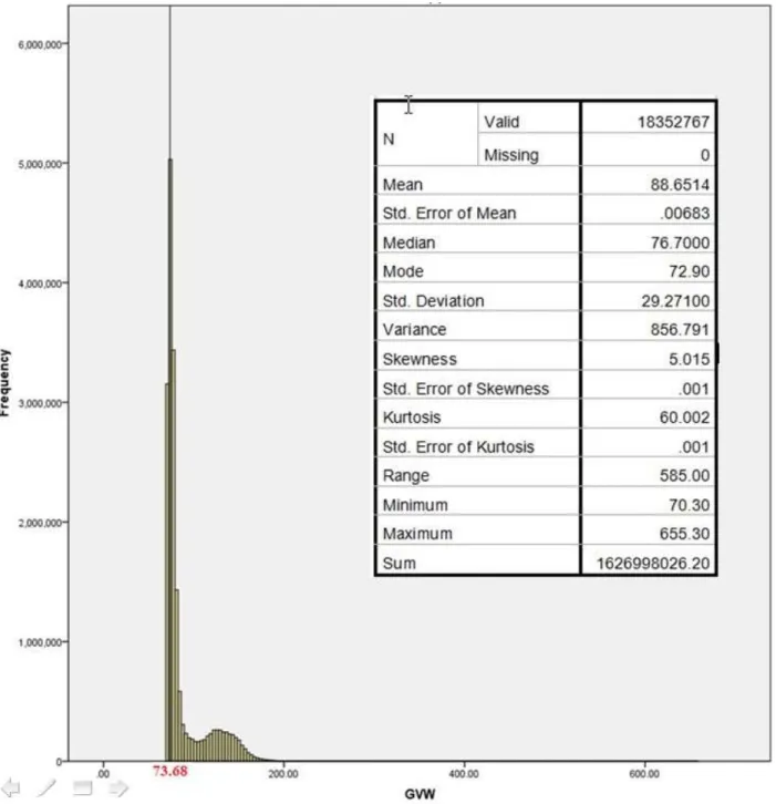
Multiple QC checks are then used to verify data accuracy. In general, these checks include comparing truck percentages by type and GVWs found in the WIM data to historical values or manual counts, and comparing measured axle weights and configurations to reasonably expected values. The first check is to compare vehicle type percentages to expected values at the site if available. The following checks are suggested by NCHRP 683 for the common 5-axle (Class 9 or 3S2) semi-trailer truck data collected: compare the number and proportion of trucks over 100 kips to expected values; compare the mean drive axle weight to the mean values found in NCHRP Report 495 (Fu et al. 2003); compute the mean value for steering axle weight, which is typically between 9 kips and 11 kips; and check mean spacing between drive tandem axles, and compare to expected values. Finally, a histogram of GVW can be developed. The usual distribution is bi-modal, with one peak corresponding to an unloaded vehicle and the second for a loaded vehicle. These peaks can be compared to expected values (typically 30 kips unloaded and from 72 and 80 kips loaded).
Assessing the statistical adequacy of the data involves inspection of the confidence interval of the upper tail of WIM data. Because only a small sample of the entire truck population is collected from WIM data, using this limited data to model the entire population is associated with uncertainty. Of particular concern is the uncertainty associated with the upper tail (heaviest) of the truck weights. This uncertainty is statistically quantifiable with confidence interval evaluation (Ang and Tang 2007). NCHRP 683 recommends that the 95% confidence interval of the upper 5% of truck weights from the WIM data is considered. That is, what range of uncertainty is associated with critical distribution parameters such as mean value and standard deviation, to a 95% level of confidence. Here, the distribution type that best-fits, per standard goodness-of-fit tests, such as Kolmogorov-Smirnov, Chi-square, or Anderson Darling (Ang and Tang 2007), for example, the upper 5% of the Michigan WIM data is determined. Then, the appropriate confidence interval is constructed for mean value and standard deviation. Thus, the range of values representing uncertainty in the mean and standard deviation can be quantified, to a 95% confidence level. An unacceptably wide confidence interval indicates that an inadequate number of data were collected. In this case, additional data collection from these sites is recommended, or to remove the affected sites from the project database.
In NCHRP 683, several different truck placement possibilities that may cause variations in load effect were considered. Here, multiple presence statistics were generated for two “side-by-side” trucks (defined as two trucks in adjacent lanes overlapping by one-half of a truck length or more); two “staggered” trucks (two trucks with an overlap less than one-half of a truck length but a gap between them less than the bridge span); and for “multiple” trucks, where more than one truck side-by-side appears in both lanes.
Convolution was also suggested as a method to generate multiple presence effects, as described in NCHRP 683 and elsewhere (Croce and Salvatore 2001). Here, the single-lane load effect histograms are numerically integrated with the convolution equation, which provides the probability density function (PDF) of two events (i.e. two trucks side-by-side), (fxs), which is
given by:
2( 1) 1( 1) 1 ) (X f X x f x dx fxs s x s x, where and are the PDFs of truck load effects , for lanes 1 and 2. Then, from the resulting PDF, the needed statistical parameters describing two-lane load effects can be directly calculated. However, it was found by (O’Brien and Enright 2011) that since the convolution process assumes independence between truck weights in each lane, which is not necessarily correct, it can lead to misrepresentation of maximum load effects.
NCHRP 495 (Fu et al. 2003) describes a process to evaluate the effect of changing allowable truck weights on the cost of maintaining highway bridges, due to the increased damage caused by increased truck loads. In order to estimate the damage on bridge structures, a process to obtain truck weight and frequency distributions was developed, considering the data obtained from state weight stations.
2.4 MULTIPLE PRESENCE MODELING
The definition of multiple presence is not straightforward, as even holding various other factors such as ADTT and site location constant, the load effect caused by multiple presence varies greatly depending on truck headway distance in adjacent lanes, in the same lane, bridge span, and truck weight correlations as well. Some approaches ignore these complexities and model multiple presence by placing two trucks exactly side-by-side on the analysis bridge, and provide an associated occurrence probability, such as in every 1/15 or 1/30 heavy truck passages, for example, potentially based on WIM data (Moses 2001; AASHTO 2003). These multiple presence
probabilities are directly calculated from the WIM data for various important scenarios such as a ‘side-by-side’, ‘staggered’, or ’multiple’ truck scenario, for various span lengths. In this model, the precise definitions (truck headway distances and overlaps considered) used to characterize multiple presence statistics are determined based on those required to produce a significant increase in load effect over that of a single lane truck load, such as suggested by NCHRP 575 (Sivakumar et al. 2007) and others such as (Fu and You 2009; O’Brien and Enright 2011). Fu and You (2009) used this approach and considered multiple presence to occur if an adjacent truck increased the single-lane truck moment by 20% or more. Based on an analysis of WIM data from New York, they found multiple presence probabilities from 0.4 - 3.5%, as a function of ADTT and bridge span. However, this approach generally will not produce the most accurate multiple presence load effects, as typically, all relevant load information simply cannot be captured using this method, as significant variations in load effect are neglected (Sivakumar et al. 2011; O’Brien and Enright 2011).
Another approach is to directly determine multiple-lane load effects from Monte Carlo simulations of different traffic configurations statistically quantified from the WIM data, as suggested in (O’Brien and Enright 2011; Kwon et al. 2010). This approach is potentially most accurate, but is also most difficult to use and generalize to multiple locations, as a value for multiple presence probability is not directly calculated. This approach also requires a high- resolution timestamp in the WIM data of at least 1/100 second to properly capture the needed traffic patterns. For this simulation model, various truck parameters available from the WIM data are modeled as random variables (RVs), such as truck weights, speeds, and inter-vehicle gaps within and between lanes. These RVs are characterized by fitting the parameters to best-fit analytical probability distributions. In addition to the individual RV parameters, their inter-
relationships are also statistically characterized, which is done from high resolution WIM data by developing the correlation matrix between the RVs for linear relationships, or empirical copulas for more complex non-linear relationships (O’Brien and Enright 2011; Tabatabai et al. 2009).
Croce and Salvatore (2001) presented a more general theoretical stochastic traffic model to account for vehicular interactions. Their proposed model was based on a modified equilibrium renewal process of vehicle arrivals on a bridge, and formulates the problem of traffic actions in terms of the general theory of stochastic processes. An analytical expression for the cumulative distribution functions (CDF)s of the maximum load effect over a given time interval was developed under general assumptions. The resulting CDFs allowed studying multilane traffic effects, as well as the combined effects of traffic and other load actions, while accounting for arbitrary variations in traffic flow.
Later, Obrian and Caprani (2005) studied short to medium span, 2-lane bridges with opposing traffic for events involving more than two trucks simultaneously on the bridge. They statistically modeled vehicle headway distances measured from five days of WIM data collected from the two outermost lanes of a motorway near Auxerre, France. In the simulations, it was found that critical traffic load events are strongly dependent on the assumptions used for the headway distance (the time or distance between the front axle of a leading truck and the front axle of a following vehicle) and gap (the time or distance between the rear axle of the front truck and the front axle of the following truck) between successive trucks. Specifically, it was determined that mean load effect could be altered by 20% to 30% for reasonable gap choices. Headway distances were found to be a function of traffic flow, where headways of less than 1.5 seconds were insensitive to flow and could be fit well to quadratically increasing cumulative distribution functions, while headways from 1.5 to 4.0 seconds were strongly influenced by flow. Inter-truck
headway is influenced by truck driver behavior as well as the number of cars between trucks. They also determined that medium and long span bridge loads are strongly influenced by traffic congestion, where the gaps between vehicles become small and there is no significant dynamic interaction. For short span bridges, however, free-flowing traffic involving a small number of vehicles with dynamic interaction becomes more critical.
One of the most recent and sophisticated multiple presence models is given by O’Brien and Enright (O’Brien and Enright 2011), who carefully studied WIM data from European sites and found subtle but important correlations between vehicle weights, speeds and headway distances. They found that neglecting these correlations as in previous efforts could lead to errors close to 10% in maximum load effect. To properly model the multiple presence effect on a two-lane bridge, it was proposed that the truck traffic model includes three headway, or gap, distributions: in-lane gaps for each lane as well as an inter-lane gap. Moreover, inter-relationships exist between gap distance, vehicle weights, and speeds. To determine maximum lifetime load effect statistics from this model, a smoothed bootstrap simulation approach was used, which re-samples traffic scenarios based on the WIM data and uses kernel functions to introduce additional variation. They concluded that the model produced a better fit to the data than those neglecting the multi-lane correlations.
Some researchers also used PC simulation packages to model the dynamic response of heavy vehicles (Kordani et al. 2014a; Molan and Abdi 2014; Kordani et al. 2014b). Simulation modeling can be defined as another method for the studies related to dynamic effect of vehicles on highway structures; however, calibration should be considered as an important parameter and a precise modeling of driver behavior is required to increase the accuracy of outcomes.
2.5 COLLECTING AND ANALYZING WIM DATA
There are various methods for collecting and analyzing different forms of data in the literature (see (Aguwa, Olya and Monplaisir 2017; Hair, Anderson, Babin and Black 2010; Gelman, Carlin, Stern and Rubin 2014)). The Texas Department of Transportation (TxDOT) developed a procedure to determine equivalent single axle loads (ESALs) from WIM-collected traffic volume and classification data (Lee, C.E. and Souny-Slitine 1998). The system was also used to monitor weekly and monthly data trends such as the proportion of various vehicle classes and lane use. The system analyzed traffic data on-site by the WIM system computer and an Excel spreadsheet for vehicle classification and calculation of ESALs. The method used traffic volume and vehicle class data rather than axle load data directly, but found that the cumulative ESALs at a site depend on the traffic volume and axle loads.
Raz et al. (2004) proposed a data mining approach for automatically detecting anomalies in WIM data. The procedure was useful for automatically detecting unlikely and erroneously classified vehicles, and could identify hardware or software problems in WIM systems.
Monsere et al. (2008) studied methods for collecting, sorting, filtering, and archiving WIM data to permit development of long-term continuous records of high quality. The study used the WIM data archive to monitor WIM sensor health, develop loads for asphalt design and models for bridge rating and deck design. In addition, freight movement was monitored to develop volume, weight, safety, and time demands on highways. Data were analyzed and filtered to handle anomalous results. Axle load spectra and time of occurrence models was developed, and Monte Carlo techniques were used to generate load histories for pavement damage estimates. Moreover, side-by-side vehicular events were quantified using the precise time stamps available in the WIM
data. The long-term record was used to extrapolate the best possible statistical tail for single lane loading cases on bridges.
Pelphery et al. (2008) described a series suggestions for collecting and analyzing WIM data that includes filtering, sorting, quality control, as well as how to use the data in a load factor calibration process. The data were cleaned and filtered to remove records with formatting mistakes, spurious data, and other errors identified by the following criteria: a record does not follow the general format pattern; GVW less than 2 kips or greater than 280 kips; GVW differs from the sum of axle weights by more than 7%; an individual axle is greater than 50 kips; the speed is less than 10 mph or greater than 99 mph; truck length is greater than 200 ft; the sum of the axle spacing lengths are less than 7 ft or greater than the truck length; the first axle spacing is less than 5 ft or any axle spacing is less than 3.4 ft; and the number of axles is greater than 13. Note the similarities to these recommendations and those made by NCHRP 683. A conventional and modified sorting method for the WIM data were then developed and compared. The conventional method sorts vehicles based on their GVW, axle group weights, and truck length. This method accounts for the axle weights and spacing in assigning each vehicle to an appropriate weight table. The method tends to assign more vehicles to higher weight tables than the modified sort. The modified methods sort vehicles based only on their GVW and rear-to- steer axle length, and it does not account for axle groupings. This method assigns more vehicles to lower weight tables than the conventional sort. However, it produces higher coefficients of variation and hence higher live load factors, as compared to the conventional sort, as is thus more conservative overall than the conventional method. In the study, the conventional sort method was used to calculate live load factors, as this was believed to better represent the traffic regulatory and enforcement procedures used.
Additionally, only the top 20% of the truck weight data from each category was considered, as projected from the upper tail of the weight histogram.
2.6 DEVELOPMENT OF TIME-ADJUSTED LOAD EFFECT STATISTICS
From WIM data, load statistics can be directly calculated only for the period of time over which the data were collected. However, it is necessary to statistically quantify the maximum load effects caused by side-by-side events for the time period used for design or evaluation. For design, this time is taken as a 75-year return period according to LRFD (2014). Note that the life time of bridges may vary depending on load, maintenance and weather conditions (Eamon et. al 2014). For evaluation under LRFR, a 2 or 5-year return period is generally used (O’rien and Enright 2010). Various statistical projection techniques have been developed to extrapolate from WIM time periods to design and evaluation time periods.
One approach is to use extreme value theory to project the resulting side-by-side load effect (valid for the time period in which WIM data was collected) to the desired 5 (or 2) year and 75-year time periods. Probabilistically, it is known that the distribution of the largest values of events approaches Extreme Type distributions as the number of load events becomes large. For example, if the upper tail of the WIM load data best fits a normal distribution, the largest values approach an Extreme Type I (Gumbel) distribution; if the upper WIM data best fit a lognormal distribution, the largest values approach a Type II (Frechet) distribution, etc. (Ang and Tang 2007). Once the appropriate distribution is identified, statistics for the mean maximum load effect can be determined for any time period of projection using known distribution relationships. For example, as shown in (Ang and Tang 2007; Sivakumar et al. 2011), if a Type I distribution were considered, the 5-year mean maximum load (for side-by-side trucks) can be determined from: + (√ ) ∗ ∗ ln , where and are the mean and standard deviation computed from k side-by-side events
for the time longer period of time (i.e. N = k*5 if k was measured over 1 year and the desire is to project to a 5 year maximum). Similar relationships are available for the other distribution types as well.
Another projection technique is the plotting approach, where the cumulative distribution
function (CDF) of the n WIM data, given by n
x x F i x 1 ) (
, is plotted on probability paper representing a certain trial distribution type. This is done by scaling the y-axis of the data appropriately such that a straight line will result on the plot if the actual CDF exactly represents the trial distribution. Then, the upper tail of the CDF is extended to load effects representing longer periods of time, by one of various possible extrapolation techniques. This approach was used in MDOT Report RC-1466 (Fu and Van de Lindt 2006) on actual Michigan WIM data, where several distribution types and extrapolation techniques were considered, including linear and nonlinear (polynomial) regression, applied to both the tail end and the entire CDF of the data, on normal, lognormal, and extreme type probability papers. It was found that the best fit could be obtained by representing the data with an Extreme Type I (Gumbel) distribution. However, when used to extrapolate to longer time periods, this approach provided inconsistent results with the projection process used to calibrate the LRFD code, resulting in much higher predicted load effects. Using the obtained results would have required either lowering the target reliability index for Michigan bridges, or an increase in bridge design capacity to meet the target LRFD index (Fu and Van de Lindt 2006).
To avoid this problem, RC-1466 recommended the projection process used for the LRFD code calibration, in which the CDF for the projected data (to 75 years) was developed by raising the CDF of the existing data to the nth power, where n is the ratio of the projected time to the equivalent time over which the WIM data were monitored (Nowak 1999; Fu and Van de Lindt
2006): ( ) = ( ) , where ( ) is the CDF of the time of interest (e.g. 5 or 75 years) and
( ) is the CDF of the WIM data. The benefit of this method is that it allows consistency with LRFD projection, such that Michigan target reliability index need not be adjusted.
To enhance the accuracy of the projection results for any of these techniques (extreme value theory, plotting approach, or LRFD approach), Monte Carlo Simulation has been employed (O’Brien and Enright 2010; Sivakumar et al. 2011; Gindy and Nassif 2006). In this approach, additional load effect data is simulated, although it was found that it is generally not possible to generate the large number of data required to directly calculate statistics for maximum evaluation or design loads with sufficient confidence, due to the computational effort required (Sivakumar et al. 2011; O’Brien and Enright 2011). However, MCS can be used to extend the data pool for a limited time beyond which the data were collected, potentially increasing the accuracy of the projection when extrapolated to longer periods of time. This process been used successfully by a variety of researchers (O’Brien and Caparani 2005, O’Brien and Enright 2010, 2011; Groce and Salvatore 2001), and is suggested in NCHRP 683 as well (Sivakumar et al. 2011).
2.7 LOAD MODEL DEVELOPMENT FOR BRIDGE DESIGN AND RATING
Early work includes that by Ghosn and Moses (1986), who, as a precursor to Nowak (1999) used reliability analysis with data from large scale field measurements of actual truck loadings and bridge responses. The data were used to project to maximum expected live loads in the lifetime of the structure and to calculate a safety index. A target safety index was extracted from these values and a new design procedure was proposed to achieve this target index to provide uniform reliability for the spans considered. The target safety index was derived from average AASHTO performance, and it was suggested that the approach could be extended to allow rating of existing bridges where load conditions were monitored by WIM systems.
Ghosn (2000) considered a reliability-based procedure to determine the optimal allowable loads on highway bridges considering static and dynamic effects and the effect of increasing the legal load limit on bridge safety. The procedure used to select the most appropriate allowable truck weight was developed as follows: choose suitable safety criteria; select an acceptable reliability level; choose a range of typical bridges (designed with different code criteria, span lengths, configurations, material types, and capacity levels); statistically describe the safety margins of these typical bridges (including the likelihood of overloads and simultaneous truck occurrence); calibrate a new allowable truck load; check the effect of the proposed truck loads on the existing network of bridges, and; verify that the number of bridge deficiencies under the new regulation will be acceptable in terms of the additional costs required to maintain the existing bridge network. In this process, the maximum permissible live load moment would be determined by trial and error to satisfy the target safety index for all of the bridge types considered. The allowable truck loads that would produce the permissible live load envelope is then to be determined.
Rather than relying upon WIM, Fu and Hag-Elsafi (2000) suggested that live load model development could be based on granted overload permit data. They presented a method to develop live load models based on the permit data, developed associated models for assessing reliability, and proposed permit-load factors for overload checking.
Miai and Chan (2002) developed a new approach for load model development based on a ‘repeatable’ methodology for short span bridges to obtain extreme daily moments and shears in simply supported bridges and compared the results to the traditional normal probability paper approach used to form the AASHTO LRFD load model. The method involved the following steps: calculate extreme daily bending moments and shear forces based on the WIM data; analyze the data statistically for load model parameters (axle weights, gross vehicle weights and axle spacing);
divide the traffic into two types: loose and dense traffic status; use the Equivalent Base Length for modeling bridge live load models. In the procedure, Monte Carlo simulation was used to simulate the complex interactions of random parameters governing truck loads. Axle spacings were divided into internal and tandem spacings. It was found that axle spacing was best modeled with a lognormal distribution, while axle weights as well as GVW best followed an inverse normal distribution. For ‘loose’ traffic density, the maximum value of axle weight and GVW for bridge design was found to follow an Extreme Type I distribution, and a Weibull distribution for ‘dense’ traffic.
Ghosn et al. (2008) describes how site-specific truck weight and traffic data collected using WIM data can be used to obtain estimates of the maximum live load for a 75-year design life for new bridges as well as the two-year return period for capacity evaluation of an existing bridge. It was determined that data from the upper tails of WIM data histograms from several sites match normal probability distributions, a finding allowing the application of extreme value theory to obtain the statistics of maximum load effect. It was also found that average bridge reliability varies considerably from state to state, and that the reliability levels associated with two-lane load effects, as designed/rated, are significantly higher than the one-lane load effects. This occurs because of the lower number of side-by-side events as well as the lower load effect produced by two-lane events when compared to the conservative multiple presence model used to calibrate the AASHTO LRFD Code. The conservativeness of the LRFD multiple presence assumptions are demonstrated by Ghosn (2008), who considered load data found in California, and determined that the LRFD load factor would require a reduction from 1.75 to 1.2 for the two- lanes loaded case to maintain a consistent reliability level with the one-lane loaded case.
O’Brian et al. (2010) predicted lifetime maximum truck load by using Monte Carlo simulation to simulate traffic representative of measured vehicle data for a given bridge. Such parameters as gross vehicle weight, number of axles, axle spacing, distribution of GVW between axles, and inter-vehicle spacing were included as parameters in the model. The study used WIM systems at two European sites and considered three different methods of modeling GVW, based on histograms of the weight data: parametric fitting, which produced a moderately good fit for most of the GVW range, but significantly underestimated the probabilities in the critical upper tail; nonparametric fitting, which produced a reasonable fit for the range of commonly observed GVWs, but presented problems in the upper region of the histogram where observations are few and there are gaps with no measured data, and GVWs heavier than the maximum measured value cannot be simulated; and semi-parametric fitting, which had the best accuracy in the critical tail region, and was the ultimately recommended approach.
For development of the Eurocode traffic live load model, load effects were estimated by extrapolating from WIM data as well as Monte Carlo simulation. However, each lane was simulated independently (Bruls et al. 1996; O’Connor et al. 2001), limiting the multiple presence model accuracy, similar to the NCHRP 683 model.
In addition to his work on the LRFD Code calibration, Nowak (Nowak et al. 2010) recently considered load models for long-span bridges, and developed a corresponding traffic simulation model for this case. It was found that the maximum load scenario is a traffic jam in which trucks tend to line up in one lane. He noted, however, that trucks are usually separated by lighter vehicles, and in this typical situation, a single overloaded truck did not have a significant effect on total load effect.
Ghosn et al. (2011), used the simplified adjustment procedure suggested in the MBE to develop a load and resistance factor rating method for permit and legal loading for NYSDOT from WIM data. ODOT calibrated live load factors used for design from WIM data (Pelphery et al. 2006), and Wisconsin DOT statistically modeled maximum load effects from WIM data by fitting multi-modal distributions to axle loads and spacings, then using MCS with empirical copulas to model the axle load and spacing relationships (Taatabai et al. 2009).
Missouri DOT recently completed a recalibration of load factors for bridge design and rating, based on local WIM data (Kwon et. al. 2010). Assumptions in the traffic model were that: minimum headway distance is 0.5 s; the time between trucks could be modeled with a shifted exponential distribution; and that 70% of trucks were in the right lane. Maximum load effects were then assumed to follow a Gumbel distribution, and extreme value theory was used for projection to the design maximum load. Similar to previous methods used to characterize multiple presence, the loads in adjacent traffic lanes were treated as independent.
2.8 RELIABILITY ANALYSIS METHODS
For structural reliability problems with well-behaved limit state functions (i.e. generally with mild or no nonlinearities and random variable types close to normal), most probable point of failure (MPP) search or reliability index-based methods are often the first choice for reliability analysis, as they can typically achieve accurate results with much less computational effort than simulation methods such as Monte Carlo simulation (MCS) or one of the various variance reduction techniques (VRTs). The widely-used reliability-index based methods include the first- and second-order reliability methods (FORM, SORM) (Rackwitz and Fiessler 1978; Breitung 1984), with many variants presented in the literature (Chen and Lind 1983; Wu and Wirsching 1987; Fiessler et al. 1979; Hohenbichler et al. 1987; Tvedt 1990; Der Kiureghian et al. 1987;
Ayyub and Haldar 1984, among many others). VRTs such as importance sampling (Rubinstein 1981; Engelund and Rackwitz 1993) and adaptive importance sampling (Wu 1992; Karamchandani et al. 1989), also make use of the MPP concept, and can similarly lead to significant reductions in computational effort over MCS. For ill-behaved or difficult to capture responses, however, such as those which may be discontinuous, highly nonlinear, or that contain multiple ‘local’ reliability indices on the limit state boundary, the most probable point (MPP) search algorithms may fail or produce unstable or erroneous results. In such cases, one must rely upon a greatly reduced selection of techniques, primarily those from the simulation family that do not rely upon an MPP search such as MCS and its advanced variants (Au and Beck 2001; Au et al. 2007; Eamon and Charumas 2011) or stratified sampling methods (Iman and Conover 1980). An alternative common approach is approximating the true limit state function with a response surface (RS), of which many examples exist (Bucher et al. 1990; Gomes et al. 2004; Cheng et al. 2009, etc.) Point integration or point estimation techniques would also be possible, although results may be highly unreliable (Eamon et al. 2005).
The drawback of most sampling techniques is the effort required, particularly for high-reliability problems involving a computationally expensive, implicit limit state function. Similarly, for complex responses (highly nonlinear or discontinuous), it is may be difficult to develop a sufficiently accurate response surface for reliability analysis without expending considerable computational effort.
For the reliability analysis of bridge structures, various bridge characteristics may affect results, such as span length, material type, girder spacing, traffic characteristics, and number of lanes. Generally, the first order MPP methods such as FORM have been found to be sufficiently
accurate for calibration efforts (Nowak 1999). Minimum target reliability indices were set as β=3.5 for design and β=2.5 for operating evaluation (Nowak 1999; Moses 2001).
2.9 RELIABILITY BASED DESIGN OPTIMIZATION
In design optimization, stochastic uncertainty associated with load intensity, material properties, geometric dimensions, etc. is represented by random variables and propagated by mathematical models that quantify variability in responses that depend on such random variables. Probability theory is most commonly used to model stochastic uncertainty in design optimization. This combination of probabilistic modeling and mathematical design optimization framework leads to reliability-based design optimization (RBDO).
Recently, RBDO has been used as an appropriate approach for structural optimization under uncertainty. Deterministic structural optimization problem in RBDO is modified by a non-deterministic one subject to a combined set of non-deterministic and reliability-based design constraints, with a set of designs as well as random variables (Eamon and Rais-Rohani 2009).
There are multiple ways of formulating and solving an RBDO problem (Enevoldsen and Sorensen 1994; Frangopol 1995; Tu et al. 1999; Rais-Rohani and Xie 2005; Kharmanda and Olhoff 2007; Aoues and Chanteaueuf 2010, etc). In its generic form, an RBDO problem seeks to minimize an objective function f(X,Y), subject to a series of probabilistic constraints in the form
ii i a
f PG P
P X,Y 0 ; i1,Np
, side constraints on design variables
NDV , 1 ; Y Y k Y u k k l k with
T n X X X1, 2,..., X as vector of random variables. It is common
to treat the mean values of random variables
X as the design variables. In this approach, the objective function can be written as f(X,Y)a1
f(X,Y)a2
~f(X,Y), where
f and
~fand a2 denoting scalar weighting factors that can be used to balance the requirements for
efficiency and robustness in design (Rao 1992). Different approaches for the evaluation of probabilistic constraints have been developed (Enevoldsen and Sorensen 1994; Tu et al. 1999). More recently, Du and Chen (2004) proposed the replacement of each probabilistic constraint with an equivalent deterministic constraint and the decoupling of reliability analysis and design optimization in each design cycle, whereas Qu and Haftka (2004) suggested the use of a probability safety factor in modeling of each probabilistic constraint.
Various types of optimization algorithms are available. Some of these include Sequential Quadratic Programming (SQP) (Nocedal and Wright 2006), cross entropy methods (Fazlollahtabar and Olya 2013), Calculus-based gradient techniques (Goldberg and Kuo 1987), stochastic dynamic programming (Olya, Fazlollahtabar, and Mahdavi 2013; Olya 2014a; Molan and Abdi 2014), probabilistic dynamic programming with various density functions (Olya, 2014b; Olya & Fazlollahtabar, 2014) and normal density function (Olya, Shirazi, & Fazlollahtabar, 2013), Particle Swarm Optimization (PSO) (Kennedy 2011), Artificial bee colony optimization (Karaboga and Basturk 2007) and genetic algorithms. In some cases, genetic algorithms (GA) have been found to be more reliable for solving multi-objective optimization problems than other common optimization methods (Koumar et. al. 2017). Sakamoto and Oda (1993), combined a genetic algorithm and an optimality criteria method to optimize the layout and cross-sectional area of the trusses by minimizing the weight design of truss structures subjected to displacement constraint. Cors