University of Massachusetts Amherst University of Massachusetts Amherst
ScholarWorks@UMass Amherst
ScholarWorks@UMass Amherst
Doctoral Dissertations Dissertations and Theses
July 2019
Sparsity in Machine Learning: An Information Selecting
Sparsity in Machine Learning: An Information Selecting
Perspective
Perspective
Siwei FengElectrical and Computer Engineering
Follow this and additional works at: https://scholarworks.umass.edu/dissertations_2
Part of the Other Computer Engineering Commons, and the Signal Processing Commons
Recommended Citation Recommended Citation
Feng, Siwei, "Sparsity in Machine Learning: An Information Selecting Perspective" (2019). Doctoral Dissertations. 1550.
https://scholarworks.umass.edu/dissertations_2/1550
This Open Access Dissertation is brought to you for free and open access by the Dissertations and Theses at ScholarWorks@UMass Amherst. It has been accepted for inclusion in Doctoral Dissertations by an authorized administrator of ScholarWorks@UMass Amherst. For more information, please contact
SPARSITY IN MACHINE LEARNING:
AN INFORMATION SELECTING PERSPECTIVE
A Dissertation Outline Presented by
SIWEI FENG
Submitted to the Graduate School of the
University of Massachusetts Amherst in partial fulfillment of the requirements for the degree of
DOCTOR OF PHILOSOPHY May 2019
c
Copyright by Siwei Feng 2019
SPARSITY IN MACHINE LEARNING:
AN INFORMATION SELECTING PERSPECTIVE
A Dissertation Outline Presented by
SIWEI FENG
Approved as to style and content by:
Marco F. Duarte, Chair
Patrick A. Kelly, Member
Dennis L. Goeckel, Member
Jie Xiong, Member
Robert Jackson, Department Chair Electrical and Computer Engineering
ABSTRACT
SPARSITY IN MACHINE LEARNING:
AN INFORMATION SELECTING PERSPECTIVE
MAY 2019
SIWEI FENG
B.Sc., SOOCHOW UNIVERSITY
M.Sc., UNIVERSITY OF MASSACHUSETTS AMHERST Ph.D., UNIVERSITY OF MASSACHUSETTS AMHERST
Directed by: Professor Marco F. Duarte
Today we are living in a world awash with data. Large volumes of data are ac-quired, analyzed and applied to tasks through machine learning algorithms in nearly every area of science, business, and industry. For example, medical scientists analyze the gene expression data from a single specimen to learn the underlying causes of disease (e.g. cancer) and choose the best treatment; retailers can know more about customers’ shopping habits from retail data to adjust their business strategies to bet-ter appeal to customers; suppliers can enhance supply chain success through supply chain systems built on knowledge sharing. However, it is also reasonable to doubt whether all the genes make contributions to a disease; whether all the data obtained from existing customers can be applied to a new customer; whether all shared knowl-edge in the supply network is useful to a specific supply scenario. Therefore, it is crucial to sort through the massive information provided by data and keep what we
really need. This process is referred to as information selection, which keeps the information that helps improve the performance of corresponding machine learning tasks and discards information that is useless or even harmful to task performance. Sparse learning is a powerful tool to achieve information selection. In this thesis, we apply sparse learning to two major areas in machine learning – feature selection and transfer learning.
Feature selection is a dimensionality reduction technique that selects a subset of representative features. Recently, feature selection combined with sparse learning has attracted significant attention due to its outstanding performance compared with traditional feature selection methods that ignore correlation between features. How-ever, they are restricted by design to linear data transformations, a potential draw-back given that the underlying correlation structures of data are often non-linear. To leverage more sophisticated embedding than the linear model assumed by sparse learning, we propose an autoencoder-based unsupervised feature selection approach that leverages a single-layer autoencoder for a joint framework of feature selection and manifold learning. Additionally, we include spectral graph analysis on the projected data into the learning process to achieve local data geometry preservation from the original data space to the low-dimensional feature space.
Transfer learning describes a set of methods that aim at transferring knowledge from related domains to alleviate the problems caused by limited/no labeled training data in machine learnig tasks. Many transfer learning techniques have been pro-posed to deal with different application scenarios. However, due to the differences in data distribution, feature space, label space, etc., between source domain and target domain, it is necessary to select and only transfer relevant information from source domain to improve the performance of target learner. Otherwise, the target learner can be negatively impacted by the weak-related knowledge from source domain, which is referred to as negative transfer. In this thesis, we focus on two transfer learning
scenarios for which limited labeled training data are available in target domain. In the first scenario, no label information is avaible in source data. In the second scenario, large amounts of labeled source data are available, but there is no overlap between the source and target label spaces. The corresponding transfer learning technique to
the former case is called self-taught learning, while that for the latter case is called
few-shot learning. We apply self-taught learning to visual, textal, and audio data. We also apply few-shot learning to wearable sensor based human activity data. For both cases, we propose a metric for the relevance between a target sample/class and a source sample/class, and then extract information from the related samples/classes for knowledge transfer to perform information selection so that negative transfer caused by weakly related source information can be alleviated. Experimental results show that transfer learning can provide better performance with information selection.
TABLE OF CONTENTS
Page ABSTRACT. . . .iv LIST OF TABLES. . . x LIST OF FIGURES. . . .xi CHAPTER 1. INTRODUCTION . . . 11.1 Unsupervised Feature Selection . . . 1
1.2 Transfer Learning . . . 4 1.2.1 Self-Taught Learning . . . 5 1.2.2 Few-Shot Learning . . . 7 1.3 Outline . . . 8 2. BACKGROUND . . . 9 2.1 Notations . . . 9 2.2 Single-Layer Autoencoder . . . 10
2.3 Long-Short Term Memory Network . . . 11
2.4 Sparse Learning-Based Unsupervised Feature Selection . . . 12
2.5 Self-Taught Learning . . . 16
2.6 Human Activity Recognition . . . 18
2.7 Few-Shot Learning . . . 19
3. UNSUPERVISED FEATURE SELECTION. . . 21
3.1 Introduction . . . 21
3.2 Proposed Method . . . 22
3.2.1 Objective Function . . . 22
3.3 Experiments . . . 27
3.3.1 Evaluation Metric . . . 27
3.3.2 Experimental Setup . . . 29
3.3.3 Parameter Sensitivity . . . 30
3.3.4 Feature Selection Illustration . . . 34
3.3.5 Clustering Illustration . . . 34
3.3.6 Performance Comparison . . . 35
4. SELF-TAUGHT LEARNING . . . 40
4.1 Introduction . . . 40
4.2 Proposed Method . . . 41
4.2.1 Knowledge Transfer and Relevance Measure . . . 41
4.2.1.1 Objective Function . . . 41
4.2.1.2 Optimization . . . 45
4.2.2 Classifier Training . . . 48
4.2.2.1 Source Domain Sample Reweighting . . . 49
4.2.2.2 Pseudo-Labeling . . . 49 4.2.2.3 Classifier Training . . . 50 4.3 Experiments . . . 51 4.3.1 Dataset Preparation . . . 51 4.3.2 Experimental Setup . . . 54 4.3.3 Parameter Sensitivity . . . 56 4.3.4 Performance Comparison . . . 58 4.3.5 Discussion . . . 62
4.3.5.1 The Effect of Local Data Structure Preservation . . . 62
4.3.5.2 The Effect of Source Sample Selection . . . 63
5. FEW-SHOT LEARNING . . . 66 5.1 Introduction . . . 66 5.2 Proposed Method . . . 68 5.2.1 Basic Framework . . . 68 5.2.2 Implementation . . . 71 5.3 Experiments . . . 72 5.3.1 Dataset Information . . . 72
5.3.2 Source/Target Split . . . 73
5.3.3 Baselines . . . 74
5.3.4 Performance Comparison . . . 75
6. CONCLUSION AND FUTURE WORK . . . 82
6.1 Conclusion . . . 82
6.2 Future Work . . . 83
LIST OF TABLES
Table Page
3.1 Details of datasets used. . . 28 4.1 Details of datasets used in our experiment. . . 53
4.2 Performance stability of GASTL in classification with respect to
balance parameters λ and γ. Classification accuracy mean (%)
and standard deviation (%) are presented. . . 58
4.3 Performance of GASTL and competing feature selection algorithms
in classification on Caltech101 with SIFTBOW as feature.
Classification accuracy (%) is used as the evaluation metric. . . 59
4.4 Performance of GASTL and competing feature selection algorithms
in classification on Caltech101 with VGG19 as feature.
Classification accuracy (%) is used as the evaluation metric. . . 60
4.5 Performance of GASTL and competing feature selection algorithms
in classification on IMDB. Classification accuracy (%) is used as the evaluation metric. TS = Training sample number in each
target class. . . 61
4.6 Performance of GASTL and competing feature selection algorithms
in classification on Twitter. Classification accuracy (%) is used as the evaluation metric. TS = Training sample number in each
target class. . . 62
4.7 Performance of GASTL and competing feature selection algorithms
in classification on ESC-50. Classification accuracy (%) is used as the evaluation metric. . . 63 5.1 Source/target split for activities . . . 74 5.2 Network Structure for Both Datasets . . . 75
LIST OF FIGURES
Figure Page
3.1 Performance variation of the GAFS w.r.t. dimensionality of subspace
m and the percentage of features selected p(%). . . 31
3.2 Performance variation of the GAFS w.r.t. balance parametersλ and
γ. . . 33
3.3 Feature selection illustration on Yale. Each row corresponds to a
sample human face image and each column refers to percentages of features selected
p∈ {10%,20%,30%,40%,50%,60%,70%,80%,100%} from left to
right. . . 34
3.4 Clustering illustration of data embeddings on hidden layers when
hidden layer size is 2. . . 35
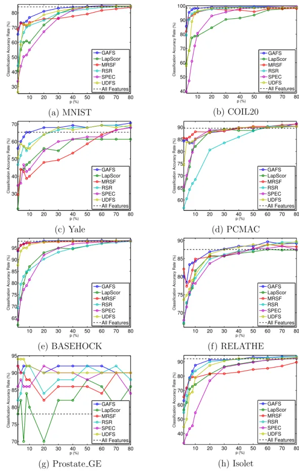
3.5 Classification accuracy w.r.t different unsupervised feature selection
algorithms and the percentage of features selectionp (%) . . . 37
3.6 Clustering accuracy w.r.t different unsupervised feature selection
algorithms and the percentage of features selectionp (%) . . . 38
3.7 Normalized mutual information w.r.t different unsupervised feature
selection algorithms and the percentage of features selection p
(%) . . . 39
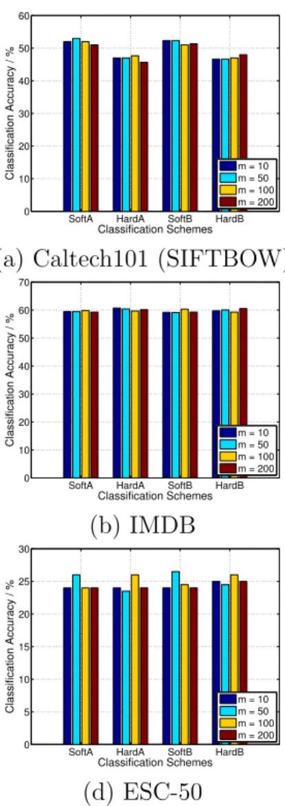
4.1 Performance of GASTL in classification as a function of the hidden
layer size m for varying sizes of the autoencoder hidden layer m.
Classification accuracy (%) is used as the evaluation metric. . . 57
4.2 Comparison of GASTL performance whenγ = 0 and optimal GASTL
performance. Classification accuracy (%) is used as the evaluation metric. Optimal values for γ are shown. . . 64
4.3 Comparison of GASTL performance when all source samples are used for classifier training and optimal GASTL performance.
Classification accuracy (%) is used as the evaluation metric.
Optimal values forp are shown. . . 65 5.1 Basic Framework . . . 68 5.2 Network Structure . . . 69
5.3 Comparison of CDHAR performance with OPP dataset. Source data
and target data are generated from the same participant.
Subfigures in the left column show results when each target class provides one training sample for target network training.
Subfigures in the right column shows results when each target class provides five training samples for target network training.
Classification accuracy (%) is used as the evaluation metric. . . 78
5.4 Comparison of CDHAR performance with OPP dataset. Source data
and target data are generated from the different participants. Subfigures in the left column show results when each target class provides one training sample for target network training.
Subfigures in the right column shows results when each target class provides five training samples for target network training.
Classification accuracy (%) is used as the evaluation metric. . . 79
5.5 Comparison of CDHAR performance with PAMAP2 dataset. Source
data and target data are generated from people from the same group. Subfigures in the left column show results when each target class provides one training sample for target network training. Subfigures in the right column shows results when each target class provides five training samples for target network training.
Classification accuracy (%) is used as the evaluation metric. . . 80
5.6 Comparison of CDHAR performance with PAMAP2 dataset. Source
data and target data are generated from people from the different groups. Subfigures in the left column show results when each target class provides one training sample for target network training. Subfigures in the right column shows results when each target class provides five training samples for target network training. Classification accuracy (%) is used as the evaluation
CHAPTER 1
INTRODUCTION
Machine learning practitioners are always yearning for training data with large volume and variety since it is believed that those can help train models with more useful information characterized and thus leading to better task performance. How-ever, in practice a large dataset is not always a guarantee for good machine learning task performance since there may exist samples and/or features that are redundant or irrelevant to specific machine learning tasks. In other words, models learned with these data may contain useless or even harmful information that negatively affect task performance. To alleviate the negative influence brought by such “bad” information, feature/sample selection is a necessary preprocessing step. Within the significant literatures on feature/sample selection, sparse learning based approaches play an im-portant role due to the selecting nature of sparse learning. In this thesis, sparse learning in unsupervised feature selection and transfer learning is investigated.
1.1
Unsupervised Feature Selection
In recent years, high-dimensional data can be found in many areas such as com-puter vision, pattern recognition, data mining, etc. Hign dimensionality enables data to include more information. However, learning high-dimensional data often suffer from several issues. For example, with a fixed number of training data, a large data dimensionality can cause the so-called Hughes phenomenon, i.e., a reduction in the generalization of the learned models due to overfitting during the training procedure compared with lower dimensional data [1]. Moreover, high-dimensional data tend to
include significant redundancy in adjacent features, or even noise, which leads to large amounts of useless or even harmful information being processed, stored, and trans-mitted [2, 3]. All these issues present challenges to many conventional data analysis problems. Moreover, several papers in the literature have shown that the intrinsic dimensionality of high-dimensional data is actually small [4–6]. Thus, dimensionality reduction is a popular preprocessing step for high-dimensional data analysis, which decreases time for data processing and also improves generalization of learned models. Feature selection [7–12] is a set of frequently used dimensionality reduction
ap-proaches that aim at selecting a subset of input dimensions1. Feature selection has
the advantage of preserving the same feature space as that of raw data. Feature selec-tion methods can be categorized into groups based on different criteria summarized below; refer to [13] for a detailed survey on feature selection.
• Label Availability. Based on the availability of label information, feature selection algorithms can be classified into supervised [7–9], semi-supervised [10– 12], and unsupervised [14–30] methods. Since labeled data are usually expensive and time-consuming to acquire [31, 32], unsupervised feature selection has been gaining more and more attention recently and is the subject of our focus in this work.
• Search Strategy. In terms of selection strategies, feature selection meth-ods can be categorized into filter, wrapper, and embedded methmeth-ods. Wrapper methods [33, 34] are seldom used in practice since they rely on a repetition of feature subset searching and selected feature subset evaluation until some stopping criteria or some desired performance are reached, which requires an exponential search space and thus is computationally prohibitive when feature dimensionality is high. Filter feature selection methods, e.g. Laplacian score
(LapScore) [14] and SPEC [15], assign a score (measuring task relevance, re-dundancy, etc.) to each feature and select those with the best scores. Though convenient to computation, these methods are often tailored specifically for a given task and may not provide an appropriate match to the specific application of interest. Embedded methods combine feature selection and model learning and provide a compromise between the two earlier extremes, as they are more efficient than wrapper methods and more task-specific than filter methods. We focus on embedded feature selection methods.
In recent years, feature selection algorithms aiming at selecting features that pre-serve intrinsic data structure (such as subspace or manifold structure) [16–30] have attracted significant attention due to their good performance and interpretability [13]. In these methods, data are linearly projected onto new spaces through a transforma-tion matrix, with fitting errors being minimized along with some sparse regulariza-tion terms. Feature importance is usually scored using the norms of corresponding rows/columns in the transformation matrix. In some methods [20–25, 28–30], the local data geometric structure, which is usually characterized by nearest neighbor graphs, is also preserved in the low-dimensional projection space. However, one basic assumption of these methods is that the data to be processed lie in or near a com-pletely linear low-dimensional manifold. However, this is not always true in practice, in particular with more sophisticated data.
We propose a novel algorithm for graph and autoencoder-based feature selection (GAFS). In this method, we integrate three objective functions into a single optimiza-tion framework: (i) we use a single-layer autoencoder to reconstruct the input data;
(ii) we use an `2,1-norm penalty on the columns of the weight matrix connecting the
autoencoder’s input layer and hidden layer to provide feature selection; (iii) we pre-serve the local geometric structure of the data through to the corresponding hidden layer activations. Extensive experiments are conducted on image data, audio data,
text data, and biological data. Many experimental results are provided to demon-strate the outstanding performance achieved by the proposed method compared with other state-of-the-art unsupervised feature selection algorithms.
The key contributions are highlighted as follows.
• We propose a novel unsupervised feature selection framework which is based on
an autoencoder and graph data regularization. By using this framework, the information of the underlying data subspace can be leveraged, which loosens the assumption of linear manifold in many relevant techniques.
• We present an efficient solver for the optimization problem underlying the
pro-posed unsupervised feature selection scheme. Our approach relies on an iterative scheme based on the gradient descent of the proposed objective function.
• We provide multiple numerical experiments that showcase the advantages of
the flexible models used in our feature selection approach with respect to the state-of-the-art approaches from the literature.
1.2
Transfer Learning
Supervised learning has excelled in many machine learning tasks such as classifi-cation [3, 35] and regression [36, 37]. However, the success of a supervised learning algorithm requires large-scale labeled training datasets and that both training and
testing data sharing the same label and feature space.2 These conditions limit the
applications of supervised learning methods in practical scenarios since it is expensive to collect eligible training data [38, 39].
Several techniques have been proposed to tackle the limitations of supervised learning methods. Semi-supervised learning [40–42] algorithms use both labeled and
unlabeled data to improve performance when labeled training data are limited. How-ever, many semi-supervised learning algorithms assume that unlabeled data and la-beled data have the same distribution [40, 41] or class labels [42]. The success of semi-supervised learning highly depends on the validity of these assumptions. How-ever, it is still difficult to gather unlabeled data which satisfy these preconditions.
In order to further loosen the restrictions on training data, many transfer learning approaches [43, 44] have been proposed. Transfer learning methods use the knowledge obtained from a source domain to improve the performance on target domain tasks. We mainly focus on two transfer learning techniques: self-taught learning and few-shot learning.
1.2.1 Self-Taught Learning
Self-taught learning [45–53] is the type of transfer learning techniques most simi-lar to semi-supervised learning, which also employs unlabeled data with the attempt to improve supervised learning performance when labeled training data are limited. However, compared with semi-supervised learning, self-taught learning methods have fewer restrictions on unlabeled data, as they allow the label spaces and marginal probability distributions of unlabeled and labeled data to be different. In self-taught learning, unlabeled data are used as source from which the knowledge learned is ap-plied to tasks performed on labeled target data. Such a loose restriction on unlabeled data significantly simplifies learning due to the huge volume of unlabeled data we can access. However, the easily obtained unlabeled data inevitably contain samples with weak relation to the labeled training data, which may even harm the supervised learning performance if we treat them equally as other unlabeled samples during knowledge transfer. This is known as negative transfer. Therefore, it is necessary to select samples that are related to the labeled data to reduce the impact caused by negative transfer.
We propose a novel algorithm for self-taught learning with unlabeled source data which are related to labeled target data to be selected. The algorithm leverages a
linear mapping, a k-nearest neighbor (kNN) graph and a single-layer autoencoder to
obtain a metric for cross domain sample relevance. We refer to this method as graph and autoencoder-based self-taught learning (GASTL). The framework of GASTL in-cludes two modules: a source sample re-weighting module and a classifier training module. In the first module, we assign each unlabeled source sample a weight that
indicates its relevance to labeled target samples.3 In the second module, source
sam-ples with large weights are selected to combine a training set with target data to train a classifier. Each selected source sample is assigned a pseudo-label from the target domain label space to be used during classifier training. The weights of source samples are also used during classifier training. The trained classifier is then used to predict labels of unseen target samples.
The key contributions are as follows:
• We propose a novel metric for the relevance of each source sample to the target
domain in the scenario of self-taught learning based on an autoencoder and graph data regularization. To the best of our knowledge, we are the first to measure source and target sample relevance for self-taught learning problems.
• We propose a novel classifier training scheme with both selected source samples
and target samples as training dataset with the relevance of each source sample to target domain being considered. We are not aware of existing self-taught learning approaches that integrate cross domain sample relevance into classifier training.
3The setting of self-taught learning requires source samples to be unlabeled and target samples
to be labeled. Therefore in the sequel we do not specify the availability of label information for both source and target samples.
• We present an efficient solver for the knowledge transfer optimization problem described above that relies on an iterative scheme based on the gradient descent of the proposed objective function. This solver shows advantages when the model complexity is large.
• Multiple experimental results are provided to demonstrate the performance
im-provements in terms of classification accuracy and insensitivity to parameters achieved by the proposed method compared with state-of-the-art self-taught learning methods and other relevant techniques.
1.2.2 Few-Shot Learning
Few-shot learning [54–56] assumes availability of labeled training data in the tar-get domain as in self-taught learning. Unlike self-taught learning, few-shot learning problems require large amounts of labeled source data whose label spaces have no overlap with that of target domain. Negative transfer also needs to be alleviated in this scenario.
We do not perform few-shot learning on multiple types of data as what we do with self-taught learning. Instead, we focus on human activity recognition with data obtained from wearable sensors such as a smartphone or wristband, which predicts activity type (e.g. walking, swimming, etc.) from the sensor outputs. Human activity recognition has been applied in many tasks such as sleep state detection [57] and smart home sensing [58].
In order to have a better discrimination of different types of activities, models need to be trained with large amounts of data from a diversity of sources. Unfortunately, in practice we do not always have enough data for each activity type. For example, a wearable health care system needs to be retrained if the previously collected activity data are not representative of the new activity type, and it is not likely for users to provide large amount of data for a single activity type. However, there may exist
relevance between new and existing activity data. Therefore, relevant knowledge from exisiting activity data can be used in model training with new data.
The algorithm we propose to perform few-shot learning on human activity recog-nition leverages a deep neural network and a linear mapping to obtain a metric for cross domain class relevance. The framework includes a feature extraction module and source class weighting module. In the first module, we use the a neural network to extract features for both source and target samples. In the second module, cross domain class similarities are measured with the features obtained in the first module and parameters of relevant source classes are used for target domain classifier train-ing. The trained classifier is then used to predict the activity type of unseen target samples.
1.3
Outline
The thesis is organized as follows.
Chapter 2 provides notations for this thesis, the concept of single-layer autoen-coder which plays an important role in algorithms described in Chapter 3 and Chapter 4, and a brief literature review of sparse learning-based unsupervised feature selection, self-taught learning, and few-shot learning. Chapter 3 presents our proposed unsu-pervised feature selection approach. Chapter 4 presents our proposed self-taught learning approach. Chap 5 presents our proposed few-shot learning approach for hu-man activity recognition. Finally, we conclude with a summary of our findings and a discussion of ongoing work in Chapter 6.
CHAPTER 2
BACKGROUND
2.1
Notations
Vectors are denoted by bold lowercase letters while matrices are denoted by bold
uppercase letters. The superscriptT of a matrix denotes the transposition operation.
For a matrix A, A(q) denotes the qth column and A
(p) denotes the pth row, while
A(p,q) denotes the entry at the pth row and qth column. The `
r,p-norm for a matrix
W∈Ra×b is denoted as kWkr,p = a X i=1 b X j=1 |W(i,j)|r !p/r 1/p . (2.1)
The trace of a matrix L∈Ra×a is defined as Tr(L) =Pa
i=1L(i,i). We use1 and 0 to
denote an all-ones and all-zeros matrix or vector of the appropriate size, respectively.
We useX= [X(1),X(2),· · · ,X(n)]∈Rd×nto denote sample sets, whereX(i) ∈Rdis
theith sample in Xfori= 1,2,· · · , n, and where dandn denote data dimensionality
and number of samples in X, respectively.
For notations in transfer learning, we use D to denote a domain andT for a task.
A domain D consists of a feature space X and a marginal probability distribution
P(X) over a sample set X. A task T consists of a label space Y and an objective
predictive function f(X,Y) to predict the corresponding labelsY of a sample set X.
We use Dsrc = {Xsrc, P(Xsrc)} and Tsrc = {Ysrc, f(Xsrc,Ysrc)} to denote the source
domain and task, and use Dtrg ={Xtrg, P(Xtrg)} and Ttrg ={Ytrg, f(Xtrg,Ytrg)} for
2.2
Single-Layer Autoencoder
A single-layer autoencoder is an artificial neural network that aims to learn a
function h(x;Θ) ≈ x with a single hidden layer, where x ∈ Rd is the input data,
h(·) is a nonlinear function, and Θ is a set of parameters. To be more specific, the
workflow of an autoencoder contains two steps:
• Encoding: mapping the input data xto a compressed data representation y∈
Rm:
y=σ(W1x+b1), (2.2)
where W1 ∈ Rm×d is a weight matrix, b1 ∈ Rm is a bias vector, and σ(·) is
an elementary nonlinear activation function. Commonly used activation func-tions include the sigmoid function, the hyperbolic tangent function, the rectified linear unit, etc.
• Decoding: mapping the compressed data representation y to a vector in the
original data space X¯ ∈Rd:
¯
X=σ(W2y+b2), (2.3)
where W2 ∈ Rd×m and b2 ∈ Rd are the corresponding weight matrix and bias
vector, respectively.
The optimization problem brought by the autoencoder is to minimize the difference between the input data and the reconstructed/output data. To be more specific,
given a set of data X = [X(1),X(2),· · · ,X(n)], the parameters W
1, W2, b1, and b2
are adapted to minimize the reconstruction error Pn
i=1kX(i) − X¯(i)k22, where X¯(i)
the reconstruction error is by selecting the parameter values via the backpropagation
algorithm.1
The data reconstruction capability of the autoencoder makes it suitable to capture the essential information of the data while discarding information that is not useful or redundant.
2.3
Long-Short Term Memory Network
A long-short term memory (LSTM) network [60] is a type of recurrent neural network (RNN) which processes time series signals by taking as their input not just the current inputs but also what they have processed earlier in time. Each RNN contains a loop (repeating modules) inside the network structure that allows information to be passed from one step of the network to the next.
RNNs show their limitations when long-term dependencies are needed to be cap-tured. Consider the task of predicting the last word in the text “I come from Jiangsu, a province in China. The closest noun “province” suggests that the last word is proba-bly the name of a country, but if we want to know which country, we need information from further back. When the gap between the position of relevant information and the point where it is needed becomes large, RNNs show their incapabilities to connect in practice.
LSTMs are a special kind of RNN, which are famous for their capabilities to cap-ture long-term dependencies. Compared with the simple repeating modules of most RNNs, which sometimes only contans a single tanh layer, the repeating modules of LSTMs include more complicated interacting layers in their structures. The work-flow of LSTM can be briefly described as follows. The first step is to determine the importance of previous information, which is to decide a status between “completely
forget about this” and “completely keep this”. The next step is to decide what new information to store in the cell state and then replace the old state with a new state. Finally, we decide the information to output.
A stacked LSTM model [61] is a LSTM model with multiple amultiple hidden LSTM layers where each layer contains multiple memory cells. By stacking LSTM hidden layers, a LSTM model can be deeper that makes it capable of tackling more complex problems.
2.4
Sparse Learning-Based Unsupervised Feature Selection
Many unsupervised feature selection methods based on subspace structure preser-vation have been proposed in the past decades. For cases missing class labels, un-supervised feature selection methods select features that are representative of the underlying subspace structure of the data [16]. The basic idea is to use a transforma-tion matrix to project data to a new space and guide feature selectransforma-tion based on the sparsity of the transformation matrix [17]. To be more specific, the generic framework of these methods is based on the optimization
min
W L(Y,WX) +λR(W), (2.4)
where Y = [Y(1),Y(2),· · · ,Y(n)] ∈ Rm×n (m < d) is an embedding matrix in which
Y(i) ∈ Rm for i = 1,2,· · · , n denotes the representation of data point X(i) in the
obtained low-dimensional subspace. L(·) denotes a loss function, andR(·) denotes a
regularization function on the transformation matrix W∈Rm×d. The methods differ
in their choice of embedding Y and loss and regularization functions; some examples
are presented below.
Multi-cluster feature selection (MCFS) [18] and minimum redundancy spectral feature selection (MRSF) [19] are two long-standing and well-known subspace
of each data X is first learned based on spectral clustering. After that, all data points are regressed to the learned embedding through a transformation matrix W ∈ Rm×d = [W(1);W(2);· · · ;W(m)]. The loss function is set to the Frobenius
norm of the linear transformation error and the regularization function is set to the
`1,1 norm of the transformation matrix, which promotes sparsity. Thus, MCFS can
be formulated mathematically as the set of separate optimization problems
min W(q)kY (q)−W(q)Xk2 2+λkW (q)k 1, (2.5)
where W(q) ∈ Rd and Y(q) ∈ Rn are the qth rows of W and Y, respectively, for
q= 1,2,· · · , m. A score for each feature is measured by the maximum absolute value of the corresponding row of the transformation matrix:
M CF S(q) = max
p=1,2,···,d|W
(p,q)|=kW(q)k∞, (2.6)
This score is then used in a filter-based feature selection scheme. MRSF is an
exten-sion of MCFS that changes the regularization function to an `2,1-norm that enforce
column sparsity on the transformation matrix. Ideally, the selected features should be representative enough to keep the loss value close to that obtained when using all
features. In order to achieve feature selection, we expect that W holds a sparsity
property with its columns, which means only a subset of the columns are nonzeros.
We use the`2-norm of a W column to measure the importance of the corresponding
feature, leading to an `2,1-norm regularization function. Furthermore, MRSF ranks
the importance of each feature according to the`2-norm of the corresponding column
of the transformation matrix. Both MCFS and MRSF are able to select features that best preserve the subspace structure of the data due to the application of spectral clustering. However, the performance of these two methods is often degraded by the separate nature of subspace learning and feature selection [29]. In order to address
this problem, many approaches on joint subspace learning and feature selection have been proposed. For example, in Gu et. al. [20] data are linearly projected to a low-dimensional subspace with a transformation matrix, and the local data geometric structure captured by a nearest neighbor graph is preserved in data embeddings on
low-dimensional subspace. In the meanwhile, an`2,1−norm is performed on
transfor-mation matrix to guide feature selection simultaneously. That is, subspace learning and feature selection are not two separate steps but combined into a single framework. Studies like [21–25] made further modifications to [20]: besides combining subspace learning and feature selection into a single framework, these methods also exploit the discriminative information of the data for unsupervised feature selection. For exam-ple, in unsupervised discriminative feature selection (UDFS) [21], data instances are
assumed to come from cclasses. UDFS uses local data geometric structure, which is
based on thek-nearest neighbor set of each data point, to incorporate local data
dis-criminative information into a feature selection framework. Like MCFS and MRFS,
UDFS also assumes the existence of a transformation matrix W ∈ Rm×c that maps
data to a low-dimensional space. The objective function of UDFS is
min
WTWTr(W
TMW) +αkWk
2,1, (2.7)
where M is an elaborate matrix that contains local data discriminative information;
see [21] for details. One drawback of these discriminative exploitation feature selection methods is that the feature selection performance relies on an accurate estimation of number of classes.
Instead of projecting data onto a low-dimensional subspace, some approaches consider combining unsupervised feature selection methods with self-representation. In these methods, each feature is assumed to be representable as a linear combination
of all (other) features, i.e.,X=WX+E, whereW∈Rd×d is a representation matrix
into the same data space so that the relationships between features can be gleaned from the transformation matrix. This type of method can be regarded as a special case of subspace learning-based feature selection methods where the embedding subspace is equal to the original space. Zhu et. al. [26] proposed a regularized self-representation (RSR) model for unsupervised feature selection that sets both the loss function and
the regularization function to`2,1-norms on the representation errorE(for robustness
to outlier samples) and transformation matrixW(for feature selection), respectively.
RSR can therefore be written as
min
W kX−WXk2,1+λkWk2,1. (2.8)
RSR has been extended to non-convex RSR [27], where the regularization function
is instead set to an `2,p-norm for 0 < p < 1. Unsupervised graph self-representation
sparse feature selection (GSR SFS) [28] further extends [27] by changing the loss function to a Frobenius norm, as well as by considering local data geometric structure
preservation on embedding WX through spectral graph analysis. GSR SFS can be
written in the following formulation
min W 1 2||X−WX|| 2 F +λ1Tr(XTWTLWX) +λ2||W||2,1, (2.9)
whereLis the graph Laplacian matrix. Lcan be calculated throughL=D−A, where
Ais the adjacency matrix which stores the similarities between vertices, andD is the
degree matrix which is a diagonal matrix containing information about the degree of vertices. Self-representation based dual-graph regularized feature selection clustering (DFSC) [29] considers the error of self-representation for both the columns and the
rows ofX(i.e., both for features and data samples). Moreover, spectral graph analysis
on both domains is considered. Subspace clustering guided unsupervised feature
with unsupervised feature selection. In addition, SCUFS also exploits discriminative information for feature selection.
2.5
Self-Taught Learning
Transfer learning methods can be classified as homogeneous and heterogeneous.
Homogeneous transfer learning methods assume Xsrc = Xtrg while heterogeneous
transfer learning methods assume Xsrc 6= Xtrg. We focus on homogeneous transfer
learning.
Self-taught learning can be categorized into the group of inductive transfer
learn-ing methods [43], in which Ttrg 6= Tsrc while the domains can be either same or
different. The idea of self-taught learning was first proposed by Raina et. al. [45] and
implemented through dictionary learning and sparse coding.2 To be more specific, a
dictionary is learned using source samples:
min D,Asrc kXsrc−DAsrck2F +β nsrc X i=1 kA(srci)k1, s.t. kD(j)k ≤1,1≤j ≤s, (2.10)
where D ∈ Rd×s is a dictionary with each column as a dictionary element, and
where each column in Asrc ∈ Rs×nsrc represents the sparse coefficient vector of the
corresponding unlabeled source sample from Xsrc ∈ Rd×nsrc. After the dictionary D
is obtained, a new labeled training set{Atrg,Ytrg}in the target domain is computed
through min Atrg kXtrg−DAtrgk2F +β ntrg X i=1 kA(trgi)k1, (2.11)
where each column in Atrg ∈ Rs×ntrg represents the sparse coefficient vector of the
corresponding labeled target sample fromXtrg ∈Rd×ntrg. Finally, a classifier is learned
2We use abbreviation STL to denote the method of [45] in the sequel, while we use the full name
on the new labeled training set by applying a supervised learning algorithm. The idea of self-taught learning has been applied in scenarios such as clustering [46], visual tracking [47], object localization [48, 49], hyperspectral image classification [50], wound infection detection [51], etc.
Wang et. al. [52] propose robust and discriminative self-taught learning (RDSTL) as an extension to STL. Compared with STL, two changes are made in order to increase the robustness of the learning model and make use of supervision information
contained in target samples. The first is to replace the `1-norm loss function used in
STL with an `2,1-norm loss function because the latter is claimed to be more robust
to noise and outliers. The second is to take advantage of label information of target
samples during learning. Assume Xk ∈ Rd×nk and Ak ∈ Rs×nk denote the samples
and corresponding sparse codes belonging to thekth class. We refer to source samples
as belonging to the 0th class and assume that the dataset X is arranged by classes
so that X = [X0,X1,· · · ,XK], where K is the total number of classes in the target
samples, with A following the same setup. Then RDSTL can be written as the
following optimization problem:
min D,AkX−DAk 2 F +β K X k=0 kATkk2,1, s.t. kD(j)k ≤1,1≤j ≤s. (2.12)
Another advantage of imposing `2,1-norm regularization on the representation
coef-ficients is that it makes the learning process insensitive to the dictionary size. This
is because sparsity on rows of A helps select basis vectors in D: a basis vector
contributes little to data representation if the `2-norm value of its corresponding
co-efficient vector is close to 0. Therefore, the final task performance should not be sensitive to the dictionary size once it is large enough.
Li et. al. [53] proposes a self-taught low-rank (S-Low) coding framework which is suitable for both clustering and classification tasks in visual learning. By imposing a low-rank constraint onto the sparse coefficient matrix, S-Low coding is claimed to be able to characterize the global structure information in the target domain. The objective function of S-Low coding is
min D,Asrc,Atrg, Esrc,Etrg kAtrgkγ1 +λ1Mγ2(Esrc) +λ2Mγ2(Etrg) +λ3kAsrck2,1, s.t.Xsrc=DAsrc+Esrc, Xtrg =DAtrg+Etrg, (2.13)
where k · kγ1 denotes the matrix γ-norm with parameter γ1 and Mγ2(·) denotes the
minimax concave penalty norm with parameterγ2. We refer readers to [53] for more
details on the roles and definitions of these two norms.
Though the self-taught learning approaches mentioned above use different schemes for knowledge transfer, they all use the whole source sample set without considering their relevance to target domain, which makes these methods potentially vulnerable to negative transfer.
2.6
Human Activity Recognition
Human activity recognition (HAR) is a technique that aims at learning high-level knowledge about human activities from the low-level sensor inputs [62]. In recent years, the growing ubiquity of sensor-equipped wearables such as smart wristbands and smartphones have significantly promoted researches regarding HAR in the field of pervasive computing [63].
Machine learning algorithms have been widely used in HAR. In the last decade, traditional machine learning tools such as Markov models [64, 65] and decision trees [66, 67] have yielded tremendous progress in HAR. However, traditional machine learning methods suffer from several limitations in HAR using wearables. Most
tra-ditional machine learning algorithms applied in HAR use manually designed features including mean, variance, and frequency, which are shallow and heavily rely on hu-man domain knowledge and experience; furthermore, they are specific to particular tasks. The drawback of these hand-crafted features is two-fold: 1. shallow features can only be used to recognize low-level activities like sitting and standing but are hardly capable for high-level activities like printing papers and attending a seminar [68]; 2. task-specific features can hardly be transferred to different environments or tasks. Therefore, traditional machine learning algorithms cannot handle complex HAR scenarios, and they require one specifically designed model for each task, which increases the time and labor cost to build HAR systems in terms of both labeled data collection and model construction.
In recent years, the application of deep learning methods to HAR has significantly alleviated the drawbacks of traditional machine learning based HAR methods. First, deep neural network can extract high-level features with little or no human design. Second, deep learning models can be reused for similar tasks, which makes HAR model construction more efficient. Different deep learning models such as deep neu-ral networks [69, 70], convolutional neuneu-ral networks [71, 72], autoencoders [73, 74], restricted Boltzmann machines [75, 76], and recurrent neural networks [77, 78] have been applied in HAR. We refer readers to [62] for more details on deep learning based HAR.
2.7
Few-Shot Learning
Few-shot learning (FSL) is a transfer learning technique that applies knowledge from existing data to data from unseen classes which do not have sufficient labeled training data for model training. For example, if we are performing a task of recog-nizing bird species from images, the number of data for some rare species of birds may be insufficient to be used for training. Then the knowledge of existing bird species
can be borrowed for the learning of new species. In this case, the machine learning problem with a classifier for bird images with insufficient amount of training data is treated as a FSL problem. If there is only one image of a bird species, this would be a one-shot learning problem.
The first work for FSL is [79], in which a variational Bayesian framework is pro-posed to represent visual object categories as probabilistic models. Existing object categories, denoted as prior knowledge, is represented as a probability density func-tion on the parameters of these models. While unseen categories, denoted as the posterior model, is obtained by updating the prior with one or more observations. Lim et al. [80] propose a sample-borrowing method for multiclass object detection that adds selected samples from similar categories to the training set in order to increase the number of training data.
In recent years, deep learning based FSL has become the mainstream of FSL due to their unparalleled performance. Initialization based methods [54, 81, 82] focus on the fine-tuning process for new tasks. Finn et al. [81] aims to learn a good initialization for new tasks. Ravi et al. [54] and Munkhdalai [82] replace the weight-update process with an external memory. Hallucination based methods [83–85] learn a data generator from the base classes and use the learned generator to hallucinate data for new classes. Hariharan et al. [83] transfers variance from base class data to new classes. Antoniou et al. [84] uses generative adversarial networks to transfer style from base classes to new classes. Wang et al. [85] integrate the generator into a meta-learning framework for transfer learning purposes. Distance metric learning based methods [55, 56, 86, 87] measure the distance between two images and take advantage of the distance to classify unseen images. Examples of distance metrics include cosine similarity [56], Euclidean distance [55], CNN-based relation module [86], and graph neural network [87].
CHAPTER 3
UNSUPERVISED FEATURE SELECTION
3.1
Introduction
Feature selection is a dimensionality reduction technique that selects a subset of representative features from highdimensional data by eliminating irrelevant and redundant features. Recently, feature selection combined with sparse learning has attracted significant attention due to its outstanding performance compared with tra-ditional feature selection methods that ignores correlation between features. These works first map data onto a low-dimensional subspace and then select features by posing a sparsity constraint on the transformation matrix. However, they are re-stricted by design to linear data transformation, a potential drawback given that the underlying correlation structures of data are often non-linear. To leverage a more sophisticated embedding, we propose an autoencoder-based unsupervised feature se-lection approach that leverages a single-layer autoencoder for a joint framework of feature selection and manifold learning. More specifically, we enforce column sparsity on the weight matrix connecting the input layer and the hidden layer, as in previous work. Additionally, we include spectral graph analysis on the projected data into the learning process to achieve local data geometry preservation from the original data space to the low-dimensional feature space. Extensive experiments are conducted on image, audio, text, and biological data. The promising experimental results validate
the superiority of the proposed method1.
3.2
Proposed Method
In this section, we introduce our proposed graph autoencoder-based unsupervised feature selection (GAFS). Our proposed framework performs broad data structure preservation through a single-layer autoencoder and also preserves local data geo-metric structure through spectral graph analysis. In contrast to existing methods that exploit discriminative information for unsupervised feature selection by impos-ing orthogonal constraints on the transformation matrix [21] or low-dimensional data representation [22, 23], GAFS does not include such constraints. More specifically, we do not add orthogonal constraints on the transformation matrix because feature weight vectors are not necessarily orthogonal with each other in real-world appli-cations [89], allowing GAFS to be applicable to a larger set of appliappli-cations [17]. Furthermore, methods posing orthogonal constraints on low-dimensional data repre-sentations makes a good estimation of number of classes necessary to obtain reliable label indicators for those algorithms; such estimation is difficult to achieve in an unsupervised framework.
3.2.1 Objective Function
The objective function of GAFS includes three parts: a term based on a single-layer autoencoder promoting broad data structure preservation; a term based on spectral graph analysis promoting local data geometric structure preservation; and a regularization term promoting feature selection. As mentioned in Chapter 2.2, a single-layer autoencoder aims at minimizing the reconstruction error between output and input data by optimizing a reconstruction error-driven loss function:
L(Θ) = 1 2n n X i=1 kX(i)−h(X(i);Θ)k22 = 1 2nkX−h(X;Θ)k 2 F, (3.1)
where Θ = [W1,W2,b1,b2], h(X;Θ) = σ(W2·σ(W1X+b1) +b2); we use the
SinceW1 is a weight matrix applied directly on the input data, each column ofW1
can be used to measure the importance of the corresponding data feature. Therefore,
R(Θ) =kW1k2,1 can be used as a regularization function to promote feature selection
as detailed in Chapter 2.4. The objective function for the single-layer autoencoder based unsupervised feature selection can be obtained by combining this regularization function with the loss function of (4.2), providing us with the optimization
min Θ 1 2nkX−h(X;Θ)k 2 F +λkW1k2,1, (3.2)
where λ is a balance parameter.
Local geometric structures of the data often contain discriminative information of neighboring data point pairs [18]. They assume that nearby data points should have similar representations. It is often more efficient to combine both broad and local data information during low-dimensional subspace learning [90]. In order to characterize
the local data geometric structure, we construct ak-nearest neighbor (kNN) graphG
on the data space. The edge weight between two connected data points is determined by the similarity between those two points. We choose cosine distance as similarity
measurement for its simplicity. Therefore the adjacency matrix A for the graph Gis
defined as A(i,j)= X(i)TX(j) kX(i)k 2kX(j)k2 if X(i) ∈ Nk(X(j)) or X(j) ∈ Nk(X(i)), 0 otherwise, (3.3)
where Nk(X(i)) denotes the k-nearest neighborhood set for X(i), and X(i)
T
refers to
the transpose of X(i). The Laplacian matrix L of the graph G is defined as L =
D−A, where D is a diagonal matrix whoseith element on the diagonal is defined as
D(i,i)=Pn
j=1A
In order to preserve the local data geometric structure in the learned subspace (i.e.,
if two data pointsX(i)andX(j)are close in original data space then the corresponding
low-dimensional representations Y(i) and Y(j) are also close in the low-dimensional
embedding space), we set up the following minimization objective:
G(Θ) = 1 2 n X i=1 n X j=1 kY(i)−Y(j)k2 2A (i,j) = 1 2 n X i=1 n X j=1 (Y(i)TY(i)−Y(i)TY(j)−Y(j)TY(i)+Y(j)TY(j))A(i,j) = n X i=1 Y(i)TY(i)D(i,i)− n X i=1 n X j=1 Y(i)TY(j)A(i,j) = Tr(Y(Θ)DY(Θ)T)−Tr(Y(Θ)AY(Θ)T) = Tr(Y(Θ)LY(Θ)T), (3.4)
where Tr(·) denotes the trace operator, Y(i)(Θ) =σ(W1x(i)+b1) fori= 1,2,· · · , n
(and we often drop the dependence onΘfor readability), andY(Θ) = [Y(1)(Θ),Y(2)(Θ),· · · ,Y(n)(Θ)].
Therefore, by combining the single-layer autoencoder based feature selection ob-jective (3.2) and the local data geometric structure preservation into consideration, the resulting objective function of GAFS can be written in terms of the following
minimization with respect to the parameters Θ= [W1,W2,b1,b2]:
ˆ Θ= arg min Θ F(Θ) = arg minΘ L(Θ) +R(Θ) +G(Θ) = arg min Θ 1 2nkX−h(X;Θ)k 2 F +λkW1k2,1+γTr(YLYT) , (3.5)
where λ and γ are two balance parameters. Filter-based feature selection is then
performed using the score function GAF S(q) =kW(1q)k2 based on the weight matrix
W1 from ˆΘ.
3.2.2 Optimization
The objective function of GAFS shown in (4.6) does not have a closed-form
toolbox [92] to solve the GAFS optimization problem. The solver requires the
gradi-ents of the objective function in (4.6) with respect to its parameters Θ.
The gradients for the loss term L(Θ) can be obtained through a back-propagation
algorithm. We defer the details for the derivation of the gradients of the error term, which are standard in the formulation of backpropagation for an autoencoder. The resulting gradients are as follows:
∂L(Θ) ∂W1 = 1 n∆2X T, ∂L(Θ) ∂W2 = 1 n∆3Y T, ∂L(Θ) ∂b1 = 1 n n X i=1 ∆2(i)= 1 n∆21, ∂L(Θ) ∂b2 = 1 n n X i=1 ∆3(i)= 1 n∆31. (3.6)
Each column ∆(2i) and ∆(3i) of ∆2 ∈Rm×n and ∆3 ∈Rd×n, respectively, contains the
error term of the corresponding data point for the hidden layer and the output layer, respectively, having entries as follows:
∆(3p,i)= ( ¯X(p,i)−X(p,i))·X¯(p,i)·(1−X¯(p,i)), ∆(2q,i)= d X p=1 W(2q,p)∆(3p,i) ! ·Y(q,i)·(1−Y(q,i)), (3.7)
for p = 1,2,· · · , d, q = 1,2,· · · , m, and i = 1,2,· · · , n, and where ¯X denotes the reconstructed data output of the autoencoder. Equation (3.7) can also be rewritten in matrix form as
∆3 = (X¯ −X)•X¯ •(1−X¯), ∆2 = (WT2∆3)•Y•(1−Y),
(3.8)
where • denotes the element-wise product operator. In the sequel, we use 1 and
0 to denote an all-ones and all-zeros matrix or vector with of the appropriate size,
The regularization term R(Θ) =kW1k2,1, whose derivative does not exist for its
ith column W(1i) when W1(i) =0 for i= 1,2,· · · , d. In this case,
∂R(Θ)
∂W1
=W1U, (3.9)
where U∈Rd×d is a diagonal matrix whoseith element on the diagonal is
U(i,i)= kW(1i)k2+ −1 , kW(1i)k2 6= 0, 0, otherwise. (3.10)
where is a small constant added to avoid overflow [29]. Since kW1k2,1 is not
dif-ferentiable at 0, we calculate the subgradient for each element in W1 in that case.
That is, for each element in W1, the subgradient at 0 can be an arbitrary value in
the interval [−1,1], and so we set the gradient to 0 for computational convenience.
In summary, the gradients for the regularization term is:
∂R(Θ) ∂W1 =λW1U, ∂R(Θ) ∂W2 =0, ∂R(Θ) ∂b1 =0, ∂R(Θ) ∂b2 =0, (3.11)
The gradients of the graph term G(Θ) = γTr(YLYT) can be obtained in a
straightforward fashion as follows: ∂L(Θ) ∂W1 = ∂Tr(γYLY T) ∂Y · ∂Y ∂Z · ∂Z ∂W1 = 2γ(YL•Y•(1−Y))XT, ∂L(Θ) ∂b1 = ∂Tr(γYLY T) ∂Y · ∂Y ∂Z · ∂Z ∂b1 = 2γ(YL•Y•(1−Y))1, ∂L(Θ) ∂W2 =0, ∂L(Θ) ∂b2 =0. (3.12)
To conclude, the gradients of the GAFS objective function with respect to Θ = [W1,W2,b1,b2] can be written as ∂F(Θ) ∂W1 = 1 n∆2X T +λW 1U+ 2γ(YL•Y•(1−Y))XT, ∂F(Θ) ∂W2 = 1 n∆3Y T, ∂F(Θ) ∂b1 = 1 n∆21+ 2γ(YL•Y•(1−Y))1, ∂F(Θ) ∂b2 = 1 n∆31 (3.13)
3.3
Experiments
In this section, we evaluate the feature selection performance of GAFS in terms of both supervised and unsupervised tasks, e.g. clustering and classification, on several benchmark datasets. We also compare GAFS with other state-of-the-art unsupervised
feature selection algorithms. To be more specific, we first select p representative
features and then perform both clustering and classification on those selected features. The performance of clustering and classification is used as the metric to evaluate
feature selection algorithms. We perform experiments on eight benchmark datasets,2
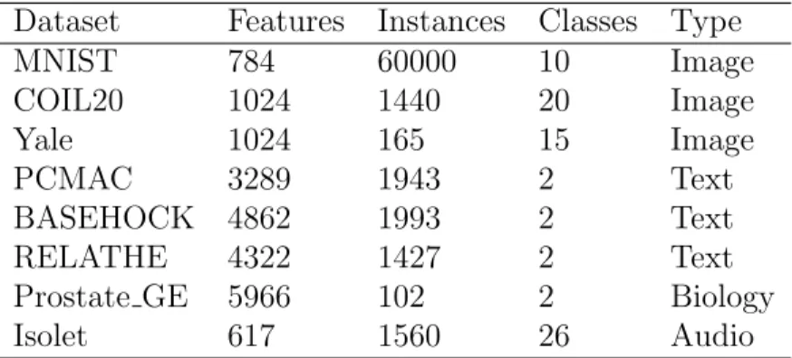
including three image datasets (MNIST, COIL20, Yale), three text datasets (PCMAC, BASEHOCK, RELATHE), one audio dataset (Isolet), and one biological dataset (Prostate GE). Detailed properties of those datasets are summarized in Table 4.1.
3.3.1 Evaluation Metric
We perform both supervised (i.e., classification) and unsupervised (i.e., cluster-ing) tasks on datasets formulated by the selected features in order to evaluate the effectiveness of feature selection algorithms. For classification, we employ softmax classifier for its simplicity and compute the classification accuracy as the evaluation
Dataset Features Instances Classes Type MNIST 784 60000 10 Image COIL20 1024 1440 20 Image Yale 1024 165 15 Image PCMAC 3289 1943 2 Text BASEHOCK 4862 1993 2 Text RELATHE 4322 1427 2 Text Prostate GE 5966 102 2 Biology Isolet 617 1560 26 Audio
Table 3.1. Details of datasets used.
metric for feature selection effectiveness. For clustering, we use k-means clustering
on the selected features and use two different evaluation metrics to evaluate the clus-tering performance of all methods. The first is clusclus-tering accuracy (ACC), defined as ACC = 1 n n X i=1 δ(gi,map(ci)),
wheren is the total number of data samples,δ(·) is defined byδ(a, b) = 1 when a=b
and 0 when a 6= b, map(·) is the optimal mapping function between cluster labels
and class labels obtained using the Hungarian algorithm [93], and ci and gi are the
clustering and ground truth labels of a given data samplexi, respectively. The second
is normalized mutual information (NMI), which is defined as
NMI = MI(C, G)
max(H(C), H(G)),
where C and G are clustering labels and ground truth labels, respectively, MI(C, G)
is the mutual information betweenC andG, andH(C) andH(G) denote the entropy
of C and G, respectively. More details about NMI are available in [94]. For both
ACC and NMI, 20 clustering processes are repeated with random initialization for each case following the setup of [18] and [21], and we report the corresponding mean values of ACC and NMI.
3.3.2 Experimental Setup
In our last experiment, we compare GAFS with LapScore3 [14], SPEC4 [15],
MRSF5 [19], UDFS6 [21], and RSR7 [26]. Among these methods, LapScore and SPEC
are filter feature selection methods which are based on data similarity. LapScore uses spectral graph analysis to set a score for each feature. SPEC is an extension to Lap-Score and can be applied to both supervised and unsupervised scenarios in which schemes of constructing graphs used for data similarity measurement are different. Details on MRSF, UDFS, and RSR can be found in Chapter 2.4. Besides the five methods, we also compare GAFS with the performance of using all features as the baseline.
Both GAFS and compared algorithms include parameters to adjust. In this exper-iment, we fix some parameters and tune others according to a “grid-search” strategy.
For all algorithms, we select p ∈ {2%, 4%, 6%, 8%, 10%, 20%, 30%, 40%, 50%,
60%, 70%, 80%} of all features for each dataset. For all graph-based algorithms,
the number of nearest neighbor in a kNN graph is set to 5. For all algorithms
pro-jecting data onto a low-dimensional space, the space dimensionality is set in the
range of m ∈ {10,20,30,40}. In GAFS, the range for the hidden layer size is set to
match that of the subspace dimensionalitym,8 while the balance parameters are given
ranges λ ∈ {10−4,10−3,10−2,10−1,1} and γ ∈ {0,10−4,5×10−4,10−3,5×10⁻³},
re-spectively. For UDFS, we use the range γ ∈ {10−9,10−6,10−3,1,103,106,109}, and λ
3Available at http://www.cad.zju.edu.cn/home/dengcai/Data/code/LaplacianScore.m 4Available at https://github.com/matrixlover/LSLS/blob/master/fsSpectrum.m 5Available at https://sites.google.com/site/alanzhao/Home
6Available at http://www.cs.cmu.edu/ yiyang/UDFS.rar 7Available at https://github.com/guangmingboy/githubs doc
8We will alternatively use the terminologies subspace dimensionality and hidden layer size in
is fixed to 103. For RSR, we use the rangeλ ∈ {10−3,5×10−3,10−2,5×10−2,10−1,5×
10−1,1,5,10,102}.
For each specific value of p on a certain dataset, we tune the parameters for each
algorithm in order to achieve the best results among all possible combinations. For classification, we report the highest classification accuracy. For clustering, we report the highest average values for both ACC and NMI from 20 repetitions.
3.3.3 Parameter Sensitivity
We study the performance variation of GAFS with respect to the hidden layer
size m and the two balance parameters λ and γ. We show the results on all the 8
datasets in terms of ACC.
We first study the parameter sensitivity of GAFS with respect to subspace
di-mensionality m. Besides the aforementioned manifold dimensionality range m ∈
{10,20,30,40}, which are common for both proposed and comparing algorithms, we
also conducted experiments with hidden layer size values of m∈ {100,200,300,400}
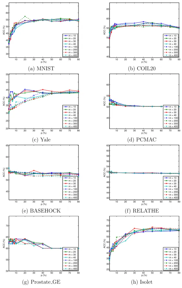
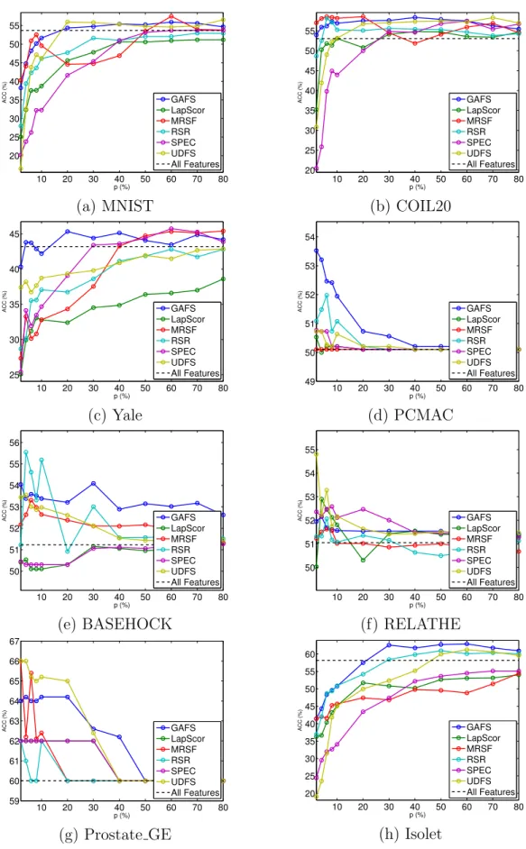
to investigate the performance change for a larger range of reduced dimensionality values. The results in Fig. 4.1 show that the performance of GAFS is not too sensi-tive to hidden layer size on the given datasets, with the exception of Yale, where the
performance with hidden layer size of m ∈ {10,20,30,40} is apparently better than
that with reduced dimensionality m ∈ {100,200,300,400}, while the performance
variations are small in the latter set. One possible reason behind this behavior is that for a human face image dataset like Yale, the differences between data instances can be subtle since they may only lie in a small area of relevance such as eyes, mouth, nose, etc. Therefore, in this case a small subspace dimensionality can be enough for information preservation, while a large subspace dimensionality may introduce redundant information that may harm feature selection performance.
10 20 30 40 50 60 70 80 30 35 40 45 50 55 60 65 p (%) ACC (%) m = 10 m = 20 m = 30 m = 40 m = 100 m = 200 m = 300 m = 400 (a) MNIST 10 20 30 40 50 60 70 80 40 45 50 55 60 65 p (%) ACC (%) m = 10 m = 20 m = 30 m = 40 m = 100 m = 200 m = 300 m = 400 (b) COIL20 10 20 30 40 50 60 70 80 20 25 30 35 40 45 50 55 p (%) ACC (%) m = 10 m = 20 m = 30 m = 40 m = 100 m = 200 m = 300 m = 400 (c) Yale 10 20 30 40 50 60 70 80 45 50 55 60 p (%) ACC (%) m = 10 m = 20 m = 30 m = 40 m = 100 m = 200 m = 300 m = 400 (d) PCMAC 10 20 30 40 50 60 70 80 45 50 55 60 65 p (%) ACC (%) m = 10 m = 20 m = 30 m = 40 m = 100 m = 200 m = 300 m = 400 (e) BASEHOCK 10 20 30 40 50 60 70 80 42 44 46 48 50 52 54 56 58 60 62 p (%) ACC (%) m = 10 m = 20 m = 30 m = 40 m = 100 m = 200 m = 300 m = 400 (f) RELATHE 10 20 30 40 50 60 70 80 50 55 60 65 70 p (%) ACC (%) m = 10 m = 20 m = 30 m = 40 m = 100 m = 200 m = 300 m = 400 (g) Prostate GE 10 20 30 40 50 60 70 80 25 30 35 40 45 50 55 60 65 70 p (%) ACC (%) m = 10 m = 20 m = 30 m = 40 m = 100 m = 200 m = 300 m = 400 (h) Isolet
Figure 3.1. Performance variation of the GAFS w.r.t. dimensionality of subspace
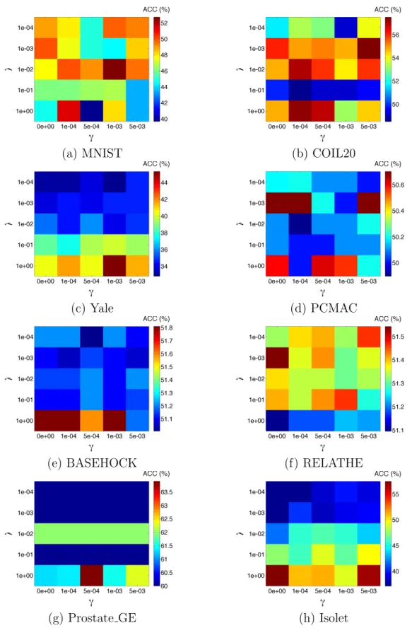
We also study the performance of GAFS on balance parameters λ and γ, with
fixed percentage of selected features and hidden layer size. We set p = 20%, as
Fig. 4.1 shows that the performance stabilizes starting at that value ofp. For subspace
dimensionality, we choosem= 10 since Fig. 4.1 shows that the performance of GAFS
is not sensitive to the value of m. The performance results are shown in Fig. 3.2,
where we find that different datasets present different trends on the ACC values
with respect to λ and γ. However, we also find that the performance differences
on PCMCA, BASEHOCK, and RELATHE are not greater than 0.8%, 0.8%, and 0.4%, respectively. Therefore we cannot make any conclusion on the influence from
two balance parameters on ACC based on these 3 datasets. For the parameter λ,
which controls the column sparsity of W1, we can find that for Yale the performance
monotonically improves as the value of λ increases for each fixed value of γ, even
though the number of selected featuresmis fixed. We believe this is further evidence
that a small number of selected features receiving large score (corresponding to large λ) is sufficient to obtain good learning performance, while having a large number of
highly scoring features (corresponding to small λ) may introduce irrelevant features
to the selection. We also find a similar behavior for Prostate GE and Isolet. For both
MNIST and COIL20, we can find that the overall performance is best when λ= 10−2
and both smaller and larger values of λ degrade the performance. This is because
the diversity among instances of these two datasets is large enough: a large value of
λ may remove informative features, while a small value of λ prevents the exclusion
of small, irrelevant, or redundant features. For the parameter γ, which controls local
data geometric structure preservation, we can find that both large values and small
values of γ degrade performance. On one hand, we can conclude that local data
geometric structure preservation does help improve feature selection performance to a certain degree. On the other hand, large weights on local data geometric structure preservation may also harm feature selection performance.
(a) MNIST (b) COIL20
(c) Yale (d) PCMAC
(e) BASEHOCK (f) RELATHE
(g) Prostate GE (h) Isolet
3.3.4 Feature Selection Illustration
We randomly select five samples from the Yale dataset to illustrate the choices
made by different feature selection algorithms. For each sample,p∈ {10%,20%,30%,40%,50%,60%,70%,80%,100%}
features are selected. Figure 3.3 shows images corresponding to the selected features
(i.e., pixels) for each sample and value of p, with unselected pixels shown in white.
The figure shows that GAFS is able to capture the most discriminative parts on human face such as eyes, nose, and mouse.
Figure 3.3. Feature selection illustration on Yale. Each row corresponds to a sample
human face image and each column refers to percentages of features selected p ∈
{10%,20%,30%,40%,50%,60%,70%,80%,100%} from left to right.
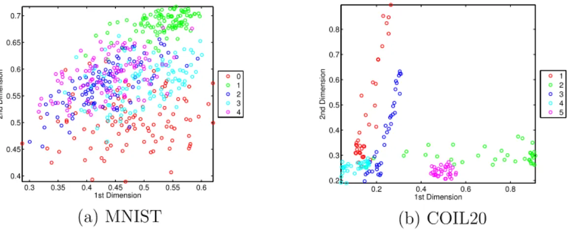
3.3.5 Clustering Illustration
We show a toy example of clustering from the low-dimensional data representation
(i.e., the hidden