A comparison of two parallel algorithms using predictive load balancing
for video compression
CARLOS-JULIAN GENIS-TRIANA
1, ABELARDO RODRIGUEZ-LEON
2and RAFAEL
RIVERA-LOPEZ
2Departamento de Sistemas y Computación
Instituto Tecnológico de Veracruz
Calzada M. A. de Quevedro 2779, Col. Formando Hogar, Veracruz, Ver.
MÉXICO
1
[email protected],
2{arleon,rrivera}@itver.edu.mx
Abstract:- This paper shows a comparison of two parallel algorithms for video compression that use predictive load balancing. One algorithm uses an exhaustive estimation of movements and the other one has an adaptive scheme. These algorithms are based on the H.264 standard of video compression and they are constructed using a Group of Pictures (GOP) level of parallelization. These algorithms are evaluated to determine their speedup when they are executed with a different number of nodes in a cluster processing videos of different types and resolutions. This evaluation is used for determining the equation that is used for calculating the number of nodes required to obtain a video compression in real time.
Key-Words: - parallel programming, load balancing, video compression.
1 Introduction
In recent years, several standards for video compression have been developed (H.264 [1], MPEG4 [2], JPEG2000 [3]), each one with advantages and drawbacks. The main challenge for video compression is to reduce the size of the transmitted video without to loss its quality. Video compression requires high performance systems that permits to reduce the compression-time, and it is in this moment that the multiprocessor systems (tightly-coupled or loosely-coupled) are required. The use of these systems (clusters by example) for video compression requires the implementation of applications using parallel programming [4]. There are several approaches for parallel programing, but Message Passing Interface (MPI) [5] is a “de facto” standard for communication among processes that model a parallel program running on a distributed memory system.
Digital video consists of a sequence of images (frames) and the effect of motion (small and continuous changes) between frames. A sequence of frames is called a "group of pictures" (GOP). In video
compression, GOPs are processed for removing the similarities between consecutive video frames or for reducing irrelevant and redundant information in frames. This redundant information is deleted for the application of predictive models, sensory redundancy or statistic redundancy [6].
Predictive model uses two methods for frame codification: intra-frame, when pixels in a frame are encoded using only the information of this frame, and
inter-frame, when a frame is encoded using the information of contiguous frames. Frames encoded using infra-frame codification are called “I-frames”, frames that are encoded using only a previously displayed reference frame are called “P-frames” and frames that are encoded using both future and previously displayed reference frames are called “ B-frames”.
This paper focuses on developing a comparison between two parallel algorithms for the video compression that use predictive load balancing. These algorithms are based on the H.264 standard of video compression and they are constructed using a parallelization of GOPs. Load distribution used in these algorithms uses two schemes: First, a pre-assignment scheme is applied for the initial allocation of GOPs in nodes of a cluster, then, an on-demand distribution scheme is applied, constructing a schedule based on the complexity analysis of encoding the next GOPs. This schedule sends a heavy GOP to the node that previously codified a lighter GOP.
These algorithms are “predictive algorithms with motion estimation”. One algorithm uses an exhaustive estimation of movements and the other one has an adaptive scheme. These algorithms are evaluated to determine their speedup when they are executed with a different number of nodes of a cluster processing videos of different types and resolutions. This evaluation is used for determining the equation that is used for calculating the number of nodes required to obtain a video compression in real time.
The rest of this paper is organized as follows. In the next section, we describe the predictive load balancing schemes used for these algorithms. Section 3 includes a description of the predictive parallel algorithm with exhaustive motion estimation. Section 4 describes the predictive parallel algorithm with adaptive motion estimation. Finally, we summarize the results of this work in Section 5.
2 Predictive load balancing schemes
The parallelization approach defined in this work uses a video stream that is divided in GOPs of 15 frames. In this approach, a GOP has the pattern IBBPBBPBBPBBP [7]. In this pattern, a “I-frame” indicates the start of a new GOP in the video sequence. The use of this pattern avoids the loss of quality produced in an inter-frame codification and it permits that each GOP can be encoded in different nodes of a cluster.2.1 Pre-assigment scheme
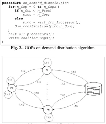
This scheme is used to assign the first group of GOPs to the nodes in a cluster. The computational cost for encoding frames is variable and unpredictable. For a cluster with n_Proc processors, each processor is identified by a number between 0 and n_Proc-1. The number of GOPs (n_Gops) is divided by n_Proc, and this value is identify as n_gop_v. Each processor receives n_gop_v GOPs for encoding. If n_Gops is not multiple of n_Proc, the remaining GOPs (n) are assigned to first n processors. Figure 1 shows a state graph for pre-assigment scheme. Table 1 shows a description of transitions in figure 1.
Fig. 1.- Pre-assigment scheme for GOPs.
2.2 On-demand distribution scheme
In an on-demand distribution scheme, the nodes of the cluster receive the next GOP when it has finished its compression. In this scheme, a dealer-node is selected for coordinating the GOP assignment to the free nodes (encoder-nodes). The objective of this scheme is to reduce the idle time in cluster processors.
Table 1.- Transitions in pre-assigment scheme.
Transition Description
T.1.1, … , T.N.1 Processor 1, …, N calculates the GOP to encode. T.1.2, …, T.N.2 Processor 1, …, N reads the GOP of disk. T.1.3, …, T.N.3 Processor 1, …, N encodes the GOP. T.1.4, …, T.N.4 Processor 1, …, N writes the encoded GOP.
In figure 2 is showed the algorithm used for this distribution scheme. Figure 3 shows a graph for the on-demand distribution scheme and table 3 shows a description of the transitions in figure 3.
procedure on_demand_distribution{ for(n_Gop = 0 to n_Gops){ if(n_Gop < n_Proc) proc = n_Gop; else proc = wait_for_Processor(); Gop_codification(proc,n_Gop); } halt_all_processors(); write_codified_Gops(); }
Fig. 2.- GOPs on-demand distribution algorithm.
Fig. 3.- GOPs on-demand distribution scheme.
3 Predictive parallel algorithm with
exhaustive motion estimation
This algorithm distributes the GOPs using a prediction process applied in each encoder-node. This algorithm uses an exhaustive motion estimation because it searches for blocks with all possible sizes used for the compression process.
Table 2.- Transitions in on-demand distribution scheme.
Transition Description
T.1.0, …, T.N.0 Processor 1, …, N notifies that is available. T.1.1, … , T.N.1 Processor 1, …, N determines the GOP to encode. T.1.2, …, T.N.2 Processor 0 notifies to processor 1, …, N the
number GOP to be encoded.
T.1.3, …, T.N.3 Processor 1, …, N reads the GOP of disk. T.1.4, …, T.N.4 Processor 1, …, N encodes the GOP. T.1.5, …, T.N.5 Processor 1, …, N writes the encoded GOP.
In this algorithm, the dealer-node (processor 0) assigns the GOPs to the encoder-nodes (processors 1, …, N). Encoder-nodes read of disk the GOP assigned and starts the compression process. Before of to finish this compression process, each encoder-node sends to the dealer-node one estimated-time for to finish its compression process.
Just before to finish the compression process in encoder-nodes, dealer-node sends the next GOP number to be codified at each encoder-node, with the aim of to reduce the idle time. This algorithm defines two elements for this prediction process: the GOP-window and the prediction scheme for the compression-time.
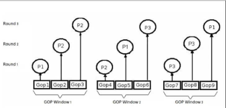
3.1 GOP-window
A “GOP-window” is the size of a group of GOPs in relation with the number of encoder-nodes. In (1) is defined the value of GOP-window (n_gop_v) when
n_Gops is the number of GOPs in the video stream and n_proc is the number of encoder-nodes in a cluster.
(1)
Each encoder-node is assigned to one GOP-window. In each step of codification process, the encoder-nodes are interchanged into the GOP-windows. The load balancing is obtained due that the allocation of encoder-node to the GOP-window is based on the computational cost of the GOP compression-time. In figure 4 is showed an example with three iterations of the assignment process, using nine GOPs grouped in three GOP-windows and using three encoder-nodes.
Fig. 4.- A example with three rounds for GOP-window assignment.
In this example, for the first round of assignment, the heavier GOP-window is the number 2, and the
lightest GOP-window is the number 1. When the first round is finished, the encoder-nodes 1 and 2 are swapped in their GOP-windows. In the second round of assignment, the heavier GOP-window is the number 3, and the lightest GOP-window is the number 2. When this round is finished, the encoder-nodes 1 and 3 are swapped in their GOP-windows.
3.2 Prediction scheme of the compression-time
For predicting the compression-time of one GOP it is necessary to use 16 frames of video stream, but only 15 frames will be stored. Frame 16 is necessary because the frame 15 is a B-frame and its uses both future and previously frames into video stream in its compression process. I-frame only uses one frame in its compression, and P-frame uses two frames in its compression. Figure 5 shows the compression sequence for the IBBPBBPBBPBBPI pattern.
Sequence 1 2 3 4 5 6 7 8 9 10 11 12 13 14 15 16 Frame Type I P B B P B B P B B P B B I B B Frame Number in GOP 0 3 1 2 6 4 5 9 7 8 12 10 11 15 13 14 Fig. 5.- Compression sequence of 16 frames.
The prediction scheme is based on sending two messages to the dealer-node:
•
Estimated-time message: The estimated-time is calculate using the average compression time of each type of frame encoded in a GOP. In the compression process, when the frame 12 is encoded, the estimated-time is calculated. The estimated-time is defined in (2).test = tIavgIr + tPavgPr + tBavgBr (2)
In (2), test is the estimated time, tIavg is the average
compression time for I-frames, Ir is the number of
I-frames uncoded, tP
avg is the average compression
time for P-frames, Pr is the number of P-frames
uncoded, tB
avgis the average compression time for
B-frames, and Br is the number of B-frames
uncoded.
•
Finish-compression message: When the encoder-node has processed the frame 15, the dealer-encoder-node is notifed that is finished. Then, the dealer-node identifies the more complex GOP-window and a encoder-node is assigned.encoder-node, the shortest estimated-time received is used by the dealer-node as a timeout for starting the scheduling process. This scheduling process assigns the encoder-nodes to the GOP-windows using the estimated-times received. Then the encoder-node that finished first is assigned to the heavier GOP-window.
Figure 6 shows a graph for predictive parallel algorithm with exhaustive motion estimation and table 4 shows a description of transitions in figure 6.
Fig. 6.- Predictive parallel scheme with exhaustive motion estimation.
Table 4.- Transitions in predictive parallel scheme with exhaustive motion estimation.
Transition Description
T.0 Processor 0 defines the GOP assignment of first round.
T.1.0, ..., T.N.0 Processor 0 notifies to processor N the number of GOP to encode.
T.1.1, … , T.N.1 Processor 1, …, N reads the GOP of disk. T.1.2, …, T.N.2 Processor 1, …, N encodes the GOP. T.1.3, …, T.N.3 Processor 1, ..., N sends its prediction-time. T.1.4, …, T.N.4 Processor 0 stores the prediction-time.
T.1.5 Processor 0 sets the Timer T.M Timer starts the scheduling.
T.0 Processor 0 defines the GOP assignment of second round.
T.1.6, …, T.N.6 Processor 1, …, N writes the encoded GOP.
4 Predictive parallel algorithm with
adaptive motion estimation
This algorithm is designed for reducing the computational time of the motion estimation [x8]. H.264 standard permits to define the characteristics of motion estimation using several parameters. Using these parameters it is possible to define several
precision
levels. In this case, three levels are used: - E0: Exhaustive search.- E1:Search using 16x16, 16x8, 8x16 and 8x8 blocks.
- E2: Search using only 16x16 blocks.
In a low-motion video, a 16x16 block is sufficient for encoding the video without quality loss. In other hand, in an high-motion video, it is necessary to explore with several blocks sizes. When a video stream is compressed using few blocks, the compression process is faster but the main problem is to define, a priori, the motion conditions in a video stream. In [8] is defined a adaptive level, identified as E-A, that uses a manual assignment of precision levels.
This algorithm was tested using two video streams (Foreman CIF and Stockholm HDTV). In figures 7, 8 and 9 are showed the comparison of compression-time, quality-loss and bit-rate increment for these adaptive levels.
Fig. 7.- Comparison of compression time.
Fig. 8.- Comparison of quality loss.
These results suggest that the use of an adaptive motion estimation is one interesting approach because it reduces the compression time (15%), and the quality-loss and the bit-rate increment are comparable with the other approaches.
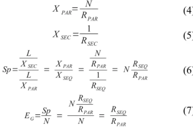
5 Performance analysis
Tests of these predictive parallel algorithms were realized in the Mozart cluster. Mozart has 4 bi-processor nodes with AMD Opteron 246 at 2 GHz interconnected by a switched Gigabit Ethernet. The video sequence used is the Riverbed HDTV. The test sequences of Riverbed have three image resolutions: 720x480, 1280x720 and 1920x1088. Each algorithm is evaluated using 2, 4 and 8 processors and their efficiency is determined (table 5). In this table, it is observed that the average efficiency is similar for all video resolutions and all number of processors. To estimate the number of processors required for real-time encoding, the average efficiency (0.9524) obtained in this analysis is used.
Table 5.- Efficiency of predictive algorithm.
Resolution 2P 4P 8P Average
720x480 0.9545 0.9638 0.9478 0.9554 1280x720 0.9527 0.9525 0.9309 0.9453 1920x1088 0.9633 0.9527 0.9536 0.9565 Average 0.9568 0.9563 0.9441 0.9524
To achieve real-time encoding in a cluster is necessary that the encoded GOPs per second is comparable with the GOPs per second generated by the video source.
The estimation of number of processor is based on the aplication of Little's law [9], showed in equation (3). In this formulation, a job is the process of to encode one GOP in one processor.
N = X*R (3)
The equation terms are:
N: Number of GOPs processed in a cluster, number of processors.
R: Compression-time of a single GOP in a cluster .
X: Number of GOPs encoded per second (compression productivity).
In this analysis, RPAR is the parallel compression
time, RSEC is the sequential compression time, L is the
number of GOPs to be encoded, Sp is the SpeedUp, EG
is the efficiency. Then, the parallel compression productivity is defined in (4), the sequential
productivity is showed in (5), the speedUp is defined in (6) and the efficiency in (7).
XPAR= N RPAR (4) XSEC= 1 RSEC (5) Sp= L XSEC L XPAR = XPAR XSEQ = N RPAR 1 RSEQ = N RSEQ RPAR (6) EG=Sp N = N RSEQ RPAR N = RSEQ RPAR (7) Using equation (7), the parallel compression time is defined in (8) and, using the Little's law, the number of processors is defined in (9). RPAR= RSEQ EG (8) N=RPARXPAR = RSEQ EG XPAR (9)
For to achieve real-time compression are needed to encode 30 frames per second (2 GOPs per second). If, by example, the sequential compression time (RSEC) for
encoding 15 frames with resolution of 720x480 is 252.06 seconds, and it is used the average efficiency for this resolution in table 5 (EG = 0.95), the number
of processors required is :
N = 252.06
0.95 2 = 531 processors
5 Conclusions
In this paper is presented a comparison between two parallel algorithms using predictive load balancing for video compression, the adaptive approach reduces 15% the compression-time in relation with the algorithm with exhaustive estimation of movements. The principal drawback of adaptive motion estimation is the complexity of determining the block size to ensure a little visible quality loss based on the conditions of movement of the video stream.
Using the Little's law, it is possible to determine the number of processor required for to produce real time compression.
As future work, it is necessary to realize more exhaustive tests for to determine the scalability of the algorithm.
References:
[1] T. Wiegand, G.J. Sullivan, G. Bjontegaard and A. Luthra: Overview of the H.264 / AVC Video Coding Standard, in IEEE Trans. on Circuits and Systems for Video Technology, vol. 13, no. 7, 2003, pp. 560-576.
[2] T. Ebrahimi, C. Horne: MPEG-4 natural video coding - An overview, in Signal Processing: Image Communication, 15, 2000, pp-365-385. [3] M. J. Gormish, D. Lee, and M.W. Marcellin:
JPEG 2000: Overview, architecture and applications, in Proc. IEEE Int. Conf. Image Processing, Vancouver, Canada, 2000, vol. II, pp. 29-32.
[4] J.C. Fernandez, M.P. Malumbres: A parallel implementation of H.26L video encoder, in
Lectures Notes on Computer Sciencies, vol. 2400, pp. 830-833, 2002.
[5] D. W. Walker: The Design of a Standard Message Passing Interface for Distributed Memory Concurrent Computers, in Parallel Computing, vol. 20, no. 4, pp. 657-673, 1994.
[6] I. E. G. Richardson: Video Coding Design, Wiley, 2002.
[7] A. Rodriguez, A. González, M.P. Malumbres.: Diseño de un Algoritmo Paralelo para codificación de Vídeo MPEG-4 sobre un cluster de Computadoras Personales, in Memorias del 9o. Congreso Internacional de Investigación en Ciencias Computacionales, Puebla, Mexico, pp. 421-430, 2002.
[8] A. Rodriguez-Leon, M. Perez, A. Gonzalez, J. Peinado, J.C. Fernandez: Paralelización del codificador H.264 con estimación de movimiento adaptiva en clusters de PCs, in Actas de las XVI Jornadas de Paralelismo, JP2005, pp. 591-597, 2005.
[9] J. D. C. Little: A Proof of the Queuing Formula: L =λW, in Operations Research, Vol. 9, No. 3, pp. 383-387, 1961.