Multi-Label Classification Models for the Prediction of Cross-Coupling Reaction Conditions

(1)

doi.org/10.26434/chemrxiv.13087769.v1

Multi-Label Classification Models for the Prediction of Cross-Coupling

Reaction Conditions

Michael Maser, Alexander Cui, Serim Ryou, Travis DeLano, Yisong Yue, Sarah Reisman Submitted date: 14/10/2020 • Posted date: 15/10/2020

Licence: CC BY-NC-ND 4.0

Citation information: Maser, Michael; Cui, Alexander; Ryou, Serim; DeLano, Travis; Yue, Yisong; Reisman, Sarah (2020): Multi-Label Classification Models for the Prediction of Cross-Coupling Reaction Conditions. ChemRxiv. Preprint. https://doi.org/10.26434/chemrxiv.13087769.v1

Machine-learned ranking models have been developed for the prediction of substrate-specific cross-coupling reaction conditions. Datasets of published reactions were curated for Suzuki, Negishi, and C–N couplings, as well as Pauson–Khand reactions. String, descriptor, and graph encodings were tested as input

representations, and models were trained to predict the set of conditions used in a reaction as a binary vector. Unique reagent dictionaries categorized by expert-crafted reaction roles were constructed for each dataset, leading to context-aware predictions. We find that relational graph convolutional networks and

gradient-boosting machines are very effective for this learning task, and we disclose a novel reaction-level graph-attention operation in the top-performing model.

File list

(2)

download file view on ChemRxiv 2020-10-13_ChemRxiv.pdf (2.25 MiB) download file view on ChemRxiv 2020-10-13_ChemRxiv_SI.pdf (3.28 MiB)

(2)

Multi-Label Classification Models for the

Prediction of Cross-Coupling Reaction Conditions

Michael R. Maser,

†,§

Alexander Y. Cui,

‡,§

Serim Ryou,

¶,§

Travis J. DeLano,

†

Yisong Yue,

‡

and Sarah E. Reisman

∗,†

†Division of Chemistry and Chemical Engineering, California Institute of Technology, Pasadena, California, USA

‡Department of Computing and Mathematical Sciences, California Institute of Technology, Pasadena, California, USA

¶Computational Vision Lab, California Institute of Technology, Pasadena, California, USA

§Equal contribution.

E-mail: [email protected]

Abstract

Machine-learned ranking models have been de-veloped for the prediction of substrate-specific cross-coupling reaction conditions. Datasets of published reactions were curated for Suzuki, Negishi, and C–N couplings, as well as Pau-son–Khand reactions. String, descriptor, and graph encodings were tested as input representa-tions, and models were trained to predict the set of conditions used in a reaction as a binary vec-tor. Unique reagent dictionaries categorized by expert-crafted reaction roles were constructed for each dataset, leading to context-aware pre-dictions. We find that relational graph convolu-tional networks and gradient-boosting machines are very effective for this learning task, and we disclose a novel reaction-level graph-attention operation in the top-performing model.

1 Introduction

A common roadblock encountered in organic synthesis occurs when canonical conditions for a given reaction type fail in complex molecule settings.1 Optimizing these reactions frequently requires iterative experimentation that can slow progress, waste material, and add significant costs to research.2 This is especially prevalent

in catalysis, where the substrate-specific nature of reported conditions is often deemed a ma-jor drawback, leading to the slow adoption of new methods.1–3 _{If, however, a transformation’s}

structure-reactivity relationships (SRRs) were well-known or predictable, this roadblock could be avoided and new reactions could see much broader use in the field.4

Machine learning (ML) algorithms have demonstrated great promise as predictive tools for chemistry domain tasks.5 Strong approaches to molecular property prediction6–9 _and

gen-erative design10–13 _{have been developed,}

par-ticularly in the field of medicinal chemistry.14 Some applications have emerged in organic synthesis, geared mainly towards predicting reaction products,15,16 yield,17–20 and selectiv-ity.21–25 _{Significant effort has also been invested}

in computer-aided synthesis planning (CASP)26

and the development of retrosynthetic design algorithms.27–30

To supplement these tools, initial attempts have been made to predict reaction conditions in the forward direction based on the substrates and products involved.31 _{Thus far, studies have}

focused on global datasets with millions of data points of mixed reaction types. Advantages of this approach include ample training data and the ability to query any transformation with a

(3)

single model. However, the sparse representa-tion of individual reacrepresenta-tions is a major drawback, in that reliable predictions can likely only be expected for the most common reactions and conditions within. This precludes the ability to distinguish subtle variations in substrate struc-tures that lead to different condition require-ments, which is critical for SRR modeling.

In recent years, it has become a goal of ours to develop predictive tools to overcome challenges in selecting substrate-specific reaction condi-tions. Towards this end, we recently reported a preliminary study of graph neural networks (GNNs) as multi-label classification (MLC)

mod-els for this task.32 We selected four high-value reaction types from the cross-coupling literature as testing grounds: Suzuki, C–N, and Negishi couplings, as well as Pauson-Khand reactions (PKRs).33 Modeling studies indicated relational graph convolutional networks (R-GCNs)34 _as

uniquely suited for our learning problem. We herein report the full scope of our studies, includ-ing improvements to the R-GCN architecture and an alternative tree-based learning approach using gradient-boosting machines (GBMs).35

2 Approach and Methods

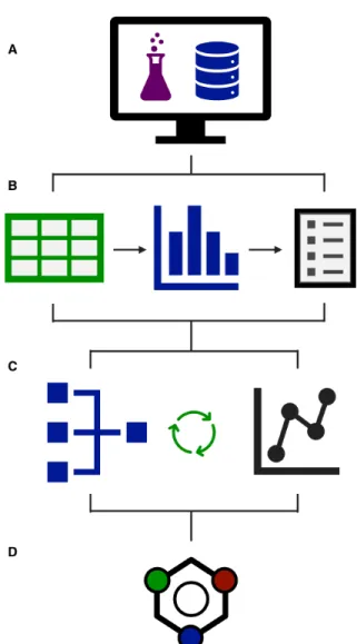
A schematic representation of the overall ap-proach is included in Figure 1. We direct the reader to our initial report32 _{for additional}

pro-cedural explanations.i

2.1 Data

acquisition

and

pre-processing

A summary of the datasets studied here is shown in Table 1. Each dataset was manually pre-processed using the following procedure:

1. Reaction data was exported from

Reaxys®query results (Figure 1A).33,36

2. SMILES strings37_{of coupling partners and}

major products were identified for each reaction entry (i.e., data point).

i_{We make our full modeling and data}

process-ing code freely available at https://github.com/ slryou41/reaction-gcnn.

Figure 1: Schematic modeling workflow. A) Data gathering. B) Tabulation and dictionary construction. C) Iterative model optimization. D) Inference and interpretation.

3. Condition labels including reagents, cat-alysts, solvents, temperatures, etc. were extracted for each data point (Figure 1B). 4. All unique labels were enumerated into a

dataset dictionary, which was sorted by reaction role and trimmed at a threshold frequency to avoid sparsity.

5. Labels were re-indexed within categories and applied to the raw data to construct binary condition vectors for each reaction. We refer to this process as binning. The reactions studied here were chosen for their ubiquity and value in synthesis, breadth 2

(4)

Table 1: Statistical summary of reaction datasets with Reaxys®queries.

name depiction reactions raw labels label bins categories

Suzuki 145,413 3,315 118 5

C–N 36,519 1,528 205 5

Negishi 6,391 492 105 5

PKR 2,749 335 83 8

of known conditions, and range of dataset size and chemical space.ii _{It should be noted that}

certain parameters (e.g. temperature, pressure, etc.) were more fully recorded in some datasets than others. In cases where this data was well-represented, reactions with missing values were simply removed, or in the case of temperature and pressure were assumed to occur ambiently. However, when appropriate, these parameters were dropped from the prediction space to avoid discarding large portions of data.

The Suzuki dataset (Table 1, line 1) was obtained from a search of C–C bond-forming reactions between C(sp2_{) halides or}

pseudo-halides and organoboron species. Data pro-cessing returned 145k reactions with 118 label bins in 5 categories. Similarly, the C–N cou-pling dataset (line 2) details reactions between aryl (pseudo)halides and amines, with 37k reac-tions and 205 bins in 5 categories. The Negishi dataset (line 3) contains C–C bond-forming reac-tions between organozinc compounds and C(sp2₎

(pseudo)halides. After processing, this dataset gave 6.4k reactions with 105 bins in 5 categories. The PKR dataset (line 4) describes couplings of C–C double bonds with C–C triple bonds to form the corresponding cyclopentenones, con-taining 2.7k reactions with 83 bins in 8 cate-gories. For all datasets, atom mapping was used as depicted in Table 1 to ensure only the desired transformation type was obtained.iii Samples of the C–N and Negishi label dictionaries are

ii_{Detailed molecular property distributions for each}

Figure 2: Samples of categorized reaction dic-tionaries for C-N and Negishi datasets.

included in Figure 2, and full dictionaries for all reactions are provided in the SI.

2.2 Model setup

For each dataset, an 80/10/10 train/validation/test split was used in modeling. Training and test sets were kept consistent between model types for sake of comparability. Model inputs were prepared as reactant/product structure tu-ples, with encodings tailored to each learning method. Models were trained using binary

dataset can be found with our previous studies.32

iii_{Given their relative frequency and to maintain}

consis-tent formatting, intramolecular couplings were dropped from the first three reactions but were retained for the PKR dataset.

(5)

Figure 3: Schematic modeling workflow. A) Tree-based methods. String and descriptor vectors for each molecule in a reaction are concatenated and used as inputs to gradient-boosting machines (GBMs). B) Deep learning methods. Molecular graphs are constructed for each molecule in a reaction, which are passed as inputs to a graph convolutional neural network (GCNN). Both model types predict probability rankings for the full reaction dictionary, which are sorted by reaction role and translated to the final output.

cross-entropy loss to output probability scores for all reagent/condition labels in the reaction dictionary (Figure 1C). The top-k ranked labels in each dictionary category were selected as the final prediction, where k is user-determined.

We define an accurate prediction as one where the ground-truth label appears in the top-k pre-dicted labels. Given the variable class-imbalance in each dictionary category,32,38 _{accuracy is}

eval-uated at the categorical level as follows:

Ac = 1 N N X i=1 1[ ˆYi∩Yi], (1)

where ˆYi and Yi are the sets of top-k predicted

and ground truth labels for the i-th sample in category c, respectively. The correct instances

are summed and divided by the number of sam-ples in the test set, N, to give the overall test accuracy in the category, or Ac.39

As a general measure of a model’s performance, we calculate its average error reduction (AER) from a baseline predictor (dummy) that always predicts the top-k most frequently occurring dataset labels in each category:

AER = 1 C C X c=1 Ag_c−Ad_c 1−Ad c , (2) whereAg

c andAdc are the accuracies of the GNN

and dummy model in the c-th category, respec-tively, and C is the number of categories in the dataset dictionary. AER represents a model’s average improvement over the naive approach

(6)

that one might use as a starting point for exper-imental optimization. In other words, AER is the percent of the gap closed between the naive model and a perfect predictor of accuracy 1.

2.3 Model construction

Both tree- and deep learning methods were ex-plored for this MLC task (Figure 3), and their individual development is discussed below.

2.3.1 Gradient-boosting machines

GBMs are decision-tree-based learning algo-rithms that are popular in the ML literature for their performance in modeling numerical data.40

We explored several string and descriptor-based encodings as numerical inputs (see SI) and found that a hybrid encoding scheme provided the greatest learnability (Figure 3A).iv _{The hybrid}

inputs are a concatenation of tokenized SMILES strings for each molecule in a reaction (coupling partners and products), further concatenated with molecular property vectors obtained from the Mordred descriptor calculator.42 _GBMs

con-sistently outperformed other tree-based learners such as random forests (RFs),43 perhaps owing to their use of sequential ensembling to improve in poor-performance regions.40

In our GBM experiments, a separate classifier was trained for all bins in a dataset dictionary, predicting whether or not they should be present in each reaction. Two general strategies have been developed for related MLC tasks, known as the binary relevance method (BM) and classifier chaining (CC).44 The BM approach considers each classifier as an independent model, predict-ing the label of its bin irrespective of the others. Conversely, CCs make predictions sequentially, taking the output of each label as an additional input for the next one, where the optimal order of chaining is a learned parameter.45 While the BM approach is significantly simpler from a com-putational perspective, CCs offer the potential for higher accuracy by modeling interdependen-cies between labels.44

iv_{Gradient boosting was implemented using}

Mi-crosoft’s LightGBM.41

We saw modeling reagent correlations as pru-dent in our studies since they are frequently observed in synthesis. Some examples relevant to this work include using a polar protic solvent with an inorganic base, excluding exogenous lig-and when using a pre-ligated metal source, set-ting the temperature below the boiling point of the solvent, etc. We decided to explore both methods, testing BM against a modern up-date to CCs introduced by Read and coworkers known as classifier trellises (CTs).46 _{In the CT}

method, instead of fully sequential propagation, models are fit in a pre-defined grid structure (the “trellis”), where the output of each

predic-tion is passed to multiple downstream classifiers at once (Figure 3A, center). This eliminates the cost of chain structure discovery, while still benefiting from nesting predictions.44

The ordering of a CT is enforced algorithmi-cally starting from a seed label, chosen randomly or by expert intervention. From Read et al.,46

the trellis is populated by maximizing the mu-tual information (MI) between source and target labels (s`) at each step (`) as follows:

s` = argmaxk∈S

X

j∈pa(`)

I(yj;yk), (3)

where S and pa(`) are the set of remaining la-bels and the available trellis structure at the current step, respectively, andyj and yk are the

j-th and k-th target labels, respectively. Here,

I(yj;yk) represents the MI between labels j and

k based on their co-occurrences in the dataset. The matrix of all pairwise label dependencies

I(Yj;Yk) is constructed as below: I(Yj;Yk) = X yj∈Yj X yk∈Yk p(yj, yk)log p(yj, yk) p(yj)p(yk) , (4) wherep(yj, yk), andp(yj) andp(yk) are the joint

and marginal probability mass functions of yj

and yk, respectively. Yj and Yk represent the

possible valuesyj andykcan each assume, which

for our task of binary classification are both {0,1}. Full MI matrices and optimized trellises for each dataset are included in the SI, and an example is discussed with the results.

(7)

2.3.2 Relational graph convolutional networks

Originally reported by Schlichtkrull et al.,34

R-GCNs are a subclass of message passing neural networks (MPNNs)47 that explicitly model re-lational data such as molecular graphs. This is achieved by constructing sets of relation op-erations, where each relation r ∈ R is specific to a type and direction of edge between con-nected nodes. In our setting, the relations oper-ate on atom-bond-atom triples using a learned, sparse weight matrixW(_rl) in each layerl.34_{In a}

propagation step, each current node representa-tionh(_il) is transformed with all relation-specific neighboring nodes h(_jl) and summed over all re-lations such that:

h(_il+1) =σ   X r∈R X j∈Nr i 1 ci,r W(_rl)h(_jl)+W(₀l)h(_il)  , (5) where Nr

i is the set of applicable neighbors and

σ is an element-wise non-linearity, for us the tanh. The self-relation termW(₀l)h(_il) is added to preserve local node information, andci,r is a

nor-malization constant.34 _{Unlike traditional GCNs,}

R-GCNs intuitively model edge-based messages in local sub-graph transformations.34 _{This is}

potentially very powerful for reaction learning in that information on edge types (i.e., single, double, triple, aromatic, and cyclic bonds) is crucial for modeling reactivity.

Here, we extend the R-GCN architecture with an additional graph attention layer (GAL) at the final readout step inspired by graph atten-tion networks (GATs) from Veliˇckovi´c48 and Busbridge.49_{As described by Veliˇ}_ckovi´_{c et al.,}48

GALs compute pair-wise node attention coeffi-cients αij for each node hi in a graph and its

neighborshj. Two nodes’ features are first

trans-formed via a shared weight matrix W, the re-sults of which are concatenated before applying a learned weight vector and softmax normaliza-tion. The final update rule is simply a linear combination of αij with the newly transformed

node vectors (Whj), summed over all

neighbor-ing nodes and averaged over a set of parallel attention mechanisms.48

In our recent studies,32 _{we observed that}

ex-isting relational GATs (R-GATs)49 _using

atom-level attention layers were less effective for our task than simple R-GCNs.v _Inspired

nonethe-less by the chemical intuition of graph atten-tion, we adapted existing GALs to construct a

reaction-level attention mechanism. Instead of pair-wise αij, we construct self-attention

coeffi-cients αm_i for all nodeshm_i in a molecular graph

hm ={hm₀ , hm₁ , ..., hm_L}. As in GATs, we take a linear combination of αm

i for all Lnodes in hm

after further transformation by matrix Wg:

αm_i =σ(Wshm_i ), ∀i∈ {1,2, ..., L}, (6)

ha_i =αm_i Wghm_i , (7) whereWsis the learned attention weight matrix,

σ is the sigmoid activation function, andha i is

the updated node representation. The convolved graphs ha ₌ _{_ha

0, ha1, ..., haL} for each molecule

m are then concatenated on the node feature axis to give an overall reaction representation

hr _{that we term the attended reaction graph}

(ARG): ARG =hr = " M

k

m=1 hma # , (8)

whereM is the number of molecules in the re-action (reactants and products) and k denotes concatenation. Similar to the attention mecha-nism above, reaction-level attention coefficients

α_ir are then constructed and linearly combined with the ARG nodes hr

i after transformation

with Wv. The final readout vector υr is

ob-tained from the attention layer by summative pooling over the nodes:

αr_i =σ(Wrhr_i), ∀i∈ {1,2, ..., H}, (9) υr = H X i=1 αr_iWvhr_i , (10)

whereH is the total number of nodes and Wris the reaction attention weight matrix. This

con-v_{We found it necessary to reduce the hidden}

dimen-sion of R-GATs to avoid excessive memory requirements relative to other GCNs,48and thus do not make a direct comparison of their performance.

(8)

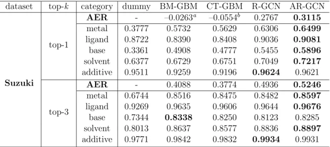
Table 2: Prediction accuracy for all model types on the Suzuki dataset.

dataset top-k category dummy BM-GBM CT-GBM R-GCN AR-GCN

Suzuki top-1 AER - –0.0263a _–0.0554b _0.2767 _0.3115 metal 0.3777 0.5732 0.5629 0.6306 0.6499 ligand 0.8722 0.8390 0.8408 0.9036 0.9081 base 0.3361 0.4908 0.4777 0.5455 0.5896 solvent 0.6377 0.6729 0.6751 0.7049 0.7217 additive 0.9511 0.9259 0.9196 0.9624 0.9621 top-3 AER - 0.4088 0.3774 0.4936 0.5246 metal 0.6744 0.8516 0.8475 0.8482 0.8597 ligand 0.9269 0.9635 0.9606 0.9644 0.9676 base 0.7344 0.8338 0.8250 0.8123 0.8285 solvent 0.8013 0.8637 0.8577 0.8836 0.8897 additive 0.9771 0.9842 0.9832 0.9934 0.9931

a_{AER excluding}_additive_{: 0.0962.} b _{AER excluding}_additive_{: 0.0922.}

struction differs from standard R-GCNs, which output readout vectors for individual molecules and concatenate them to form the ultimate re-action representation. Altogether, we term our hybrid architecture as an attended relational graph convolutional network, or AR-GCN.

In all deep learning experiments, with or with-out attention, the reaction vector readwith-outs were passed to a multi-layer perceptron (MLP) of depth = 2.vi _{The final prediction is made as}

a single output vector with one entry for each label in the reaction dictionary, and the result is translated as described in Section 2.2.

3 Results and discussion

3.1 Model performance

Our modeling pipeline was first tested on the Suzuki coupling dataset, the largest of the four. Table 2 summarizes top-1 and top-3 categori-cal accuracies (Equation 1) and AERs (Equa-tion 2) for the following models: GBMs with no trellising (BM-GBM), GBMs with trellis-ing (CT-GBM), standard R-GCNs as reported by Schlichtkrull et al. (R-GCN),32,34 our AR-GCNs developed here (AR-GCN), and the dummy predictor as a baseline (dummy).

vi_{All NN models were implemented using the Chainer}

Chemistry (ChainerChem) deep learning library.50

For this dataset, GCN models significantly outperformed GBMs across categories for both top-1 and top-3 predictions. While GBMs ac-tually gave negative top-1 AERs over baseline, these scores were dominated by the additive

contribution; excluding this category the BM-and CT-GBMs gave modest 10% BM-and 9% AERs, respectively. Despite struggling with top-1 pre-dictions, GBMs gave significant AERs for top-3, with BM-GBMs at 41% and CT-GBMs at 38%. The AR-GCNs gave the best accuracy of all models, providing 31% and 52% top-1 and top-3 AERs, respectively. AR-GCNs gave roughly 3% AER gain over the R-GCN in both top-1 and top-3 predictions, demonstrating the value of the added attention layer.

A few interesting categorical trends can be seen across model types. For instance, models provide the best error reduction (ER = A

g c−Adc

1−Ad c ,

see Equation 2) in the metal category, with the AR-GCN at 44% and 57% for top-1 and top-3, respectively. Similarly, models perform well in thebase category, where the AR-GCN gave the best top-1 ER and BM-GBMs gave the best top-3 ER. Less consistent ERs between top-1 and top-3 predictions were obtained for the remaining three categories. For example, withsolvents, the AR-GCN improved baseline by 23% in top-1 predictions, but 44% in top-3. Likewise, for AR-GCNligand predictions, a 28% ER was obtained for top-1 versus a 56% gain 7

(9)

Table 3: Prediction accuracy for all model types on the C–N, Negishi, and PKR datasets.

dataset top-k category dummy BM-GBM CT-GBM R-GCN AR-GCN

C–N top-1 AER - –0.0413a _–0.1593b _0.3453 _0.3604 metal 0.2452 0.4825 0.4582 0.5989 0.6162 ligand 0.5219 0.5538 0.5710 0.6981 0.7068 base 0.2479 0.5028 0.5003 0.5932 0.6066 solvent 0.3219 0.4582 0.4524 0.5647 0.5674 additive 0.8904 0.7669 0.7031 0.8984 0.8997 top-3 AER - 0.3568 0.3131 0.5391 0.5471 metal 0.6526 0.7928 0.7772 0.8479 0.8490 ligand 0.6647 0.7933 0.7928 0.8605 0.8688 base 0.6400 0.8008 0.7916 0.8452 0.8370 solvent 0.5677 0.7370 0.7281 0.7973 0.7997 additive 0.9156 0.9290 0.9184 0.9534 0.9559 Negishi top-1 AER - 0.3510 0.2773 0.4439 0.4565 metal 0.2887 0.5444 0.5218 0.6555 0.6730 ligand 0.7879 0.8174 0.7900 0.8724 0.8772 temperature 0.3317 0.6656 0.6527 0.6188 0.6507 solvent 0.6938 0.8562 0.8514 0.8868 0.8915 additive 0.8309 0.8691 0.8401 0.8724 0.8644 top-3 AER - 0.5947 0.5199 0.6590 0.6833 metal 0.5008 0.7771 0.7674 0.8086 0.8517 ligand 0.8549 0.9548 0.9321 0.9522 0.9553 temperature 0.5885 0.9031 0.8772 0.8517 0.8708 solvent 0.8788 0.9321 0.9402 0.9537 0.9537 additive 0.9043 0.9548 0.9354 0.9761 0.9729 PKR top-1 AER - 0.4396 0.4010 0.3973 0.4199 metal 0.4302 0.7901 0.7786 0.7132 0.7057 ligand 0.8792 0.9351 0.9237 0.9057 0.9094 temperature 0.2830 0.5954 0.5649 0.6528 0.6642 solvent 0.3321 0.6183 0.6260 0.6792 0.6981 activator 0.6906 0.8244 0.8015 0.8415 0.8491 CO (g) 0.7245 0.8855 0.8855 0.8717 0.8868 additive 0.9057 0.9008 0.8893 0.8906 0.8491 pressure 0.6528 0.8588 0.8702 0.8491 0.8491 top-3 AERc _- _0.6987 _0.6740 _0.6844 _0.7145 metal 0.7132 0.9351 0.9313 0.9057 0.8906 ligand 0.9019 0.9962 0.9924 0.9849 0.9962 temperature 0.5962 0.8740 0.8321 0.8528 0.8604 solvent 0.5925 0.8779 0.8550 0.8679 0.8981 activator 0.8830 0.9466 0.9275 0.9774 0.9774 CO (g) 1.0000 1.0000 1.0000 1.0000 1.0000 additive 0.9321 0.9885 0.9885 0.9698 0.9736 pressure 0.9623 0.9771 0.9847 0.9849 0.9849

a_{AER excluding} _additive_{: 0.2302.} b _{AER excluding}_additive_{: 0.2282.} c _Excludes _CO(g)_.

(10)

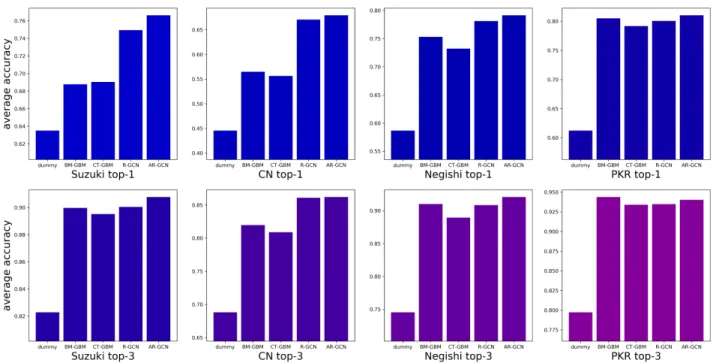
Figure 4: Average top-1 and top-3 categorical accuracies for each model across the four datasets.

in top-3. Finally, although the baseline additive

accuracy is high as the majority of reactions are null in this category, the AR-GCN still gave a 23% top-1 ER and a 70% top-3 ER.

The trends and differences between top-1 and top-3 performance gains are reflective of the fre-quency distributions in each label category.32 These intuitively resemble long-tail or Pareto-type distributions,51 _{with the bulk of the}

cumu-lative density contained in a small number of bins and the remaining bins supporting smaller frequencies. The distribution shapes are likely to influence the relative top-1 and top-3 AERs, where the highly skewed distributions could be more difficult to improve over baseline.

Having demonstrated the utility of our pre-dictive framework, we turned to the remaining datasets to assess its scope. Modeling results for C–N, Negishi, and PKRs are detailed in Table 3 and Figure 4. Notable observations for each dataset are discussed below.

C–N coupling. Similar to the Suzuki results, the AR-GCN was the top performer for C–N couplings in almost all categories, and slightly higher AERs were observed overall. The AR-GCN afforded 36% and 55% 1 and top-3 AERs, respectively, again providing slight

gains over R-GCNs at 35% and 54%. As

above, GBMs struggled with this relatively large

dataset (36,519 reactions) due to difficulties with theadditive category. Models again made strong improvements in the metal and base categories, but also gave consistently strong gains for lig-ands and solvents, especially for top-3 predic-tions. For example, the AR-GCN returned top-3 ERs of 57% for metals, 61% for ligands, 55% forbases, and 54% forsolvents. Note that these ERs correspond to very high accuracies (Ac) of

85%, 87%, 84%, and 80%, respectively.

Negishi coupling. The highest AERs of all modeling experiments came with the Negishi dataset. The AR-GCN again gave the strongest performance, with top-1 and top-3 AERs of 46% and 68%, respectively. However, the R-GCN and even GBM models gave the highest accura-cies in some categories. Interestingly, BM- and CT-GBMs performed significantly better than the GCNs for temperature predictions, though the strongest ER for most models came from the solvent category.

PKR. For the PKR dataset—the smallest of the four—simple BM-GBMs gave the best top-1 AER at 44%, followed closely by the AR-GCN at 42%. Similarly for top-3 predictions, these models gave AERs of 70% and 71%, respec-tively. Compared to the other reactions, GCNs are perhaps more prone to overfitting this small of a dataset,52making tree-based modeling more

(11)

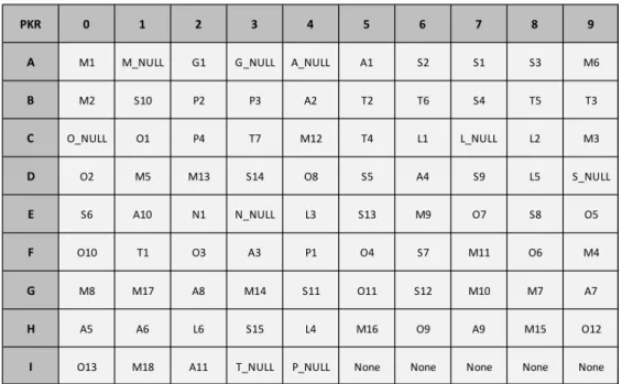
Figure 5: Optimized prediction trellis for the Suzuki dataset.

suitable. It is interesting to note that in gen-eral for PKRs, the GCN models were better at predicting physical parameters like tempera-ture, solvent, and CO(g) atmosphere, whereas GBMs gave better performance for reaction com-ponents such as metal, ligand, and additive.

3.2 Interpretability

3.2.1 Tree methods

Given the results described above, we sought an understanding of the chemical features in-forming our predictions. Tree-based learning is often favored in this regard in that feature im-portances (FIs) can be directly extracted from models. We found that FIs for our GBMs were roughly uniform across the SMILES regions of the encodings. The most informative physical descriptors from the Mordred vectors pertained to two classes: topological charge distributions53

correlated with local molecular dipoles; and Moreau–Broto autocorrelations54 weighted by polarizability, ionization potential, and valence electrons (see SI for detailed rankings). The latter class is particularly intriguing as they are calculated from molecular graphs in what have been described as atom-pair convolutions,55 _not

unlike the GCN models used here.34

An advantage to using CTs is the ability to extract their MI matrices and trellis structures for interpretation.46 The optimized trellis for the Suzuki CT-GBMs is included in Figure 5, where several chemically intuitive features and

category blocks can be noted:

1. Block A0–B4 (blue): The result of M1 (Pd(PPh3)4) is used to predict three more

metals: M2(Pd(OAc)2), M4(Pd(dppf)Cl₂·

DCM), andM5 (Pd(PPh3)2Cl2). Based on

these metal complexes, the probability of using exogenous ligand (L NULL) and L1 (PPh3) is then predicted.

2. Block C0–F2 (green): The use of unligated M6 (Pd2(dba)3) informs the predictions of

ligandsL3 (XPhos),L7 ([(t-Bu)3PH]BF4),

and L13 (Me_{CgPPh). These in turn feed}

the model of unligated M8 (Pd(dba)2),

which then informs L5 (P(o-tolyl)3).

3. Block A6–B9 (purple): Several solvents are connected, where the predictions of S4 (1,4-dioxane) and S7 (PhMe) propagate through S9 (H2O), S2 (EtOH), and S6

(MeCN). These additionally feed classifiers of S1 (THF) and S NULL(neat).

4. Block C7–F8 (red): Four different classes of base are interwoven, includingB6 (CsF) and B13 (KOt-Bu). This informs the pre-diction of B28(LiOH·H2O), which then

goes on to feed models of B18 (DIPEA) and B16 (NaOt-Bu).

As a control experiment,vii_{we withheld the}

prop-agated predictions from the CT-GBMs to test whether the MI was actually being used.56 In-deed, model accuracy dropped off markedly, even below baseline in some categories. While this suggests that CT-GBMs do learn reagent correlations, the sharp performance loss may also indicate overfitting to this information.46

Further studies are necessary to uncover the optimal molecule featurization in combination with CTs, though the results here suggest their promise in modeling structured reaction data.

3.2.2 Deep learning methods

For AR-GCNs, a valuable interpretability fea-ture lies in the learned feafea-ture weightsαr

i

(Equa-tion 9). Intuitively, the weights represent the

vii_{Detailed adversarial control studies for all GBM}

models are included in the SI.56

(12)

Figure 6: AR-GCN attention weight visualization and prediction examples from randomly chosen reactions in each dataset. Darker highlighting indicates higher attention.

model’s assignment of importance on an atom, as they re-scale node features in the final graph layer before inference. When extracted, the weights can be mapped back onto a molecule’s atoms and displayed by color scale using RDKit (Figure 1D).57 _{This gives a visual interpretation}

of the functional groups most heavily informing the predictions. Example visualizations from a random reaction in each dataset and their AR-GCN predictions are included in Figure 6, and several additional random examples for each reaction type can be found in the SI.

In the Suzuki example (Figure 6A), the atten-tion is dominated by the sp3 carbon bearing the Bpin group, with additional contributions from the bis-o-substituted heteroaryl-chloride and its cinnoline nitrogen, all of which could be reason-ably expected to influence reactivity. It is in-teresting that weights on the o-difluoromethoxy

group, the sulfone, and the majority of the prod-uct are suppressed, perhaps indicating that an alkyl nucleophile is sufficient to predict the re-quired conditions. The AR-GCN predictions are correct in each category besides the metal, where the model erroneously identifies the metal source Pd(dppf)Cl2 instead of its ground truth

DCM adduct Pd(dppf)Cl₂·DCM.

Conversely, the weights in the C–N coupling example are more evenly distributed (Figure 6B). Intuitively, the chemically active iodonium ben-zoate is given strong attention in the electrophile, as is the nucleophilic aniline nitrogen. Here, the

m-tetrafluoroethoxy group is also weighted sig-nificantly and these groups are given similar attention in the product. All categories are pre-dicted correctly in this example, though three of them are null.

The Negishi example (Figure 6C) is an inter-11

(13)

esting C(sp3_)–C(sp2_{) coupling of a fully}

substi-tuted alkenyl-iodide and thiophenyl-methylzinc chloride. Like with A, the strongest weights cor-respond to the sp3 _{nucleophilic carbon, though}

similarly strong attention is distributed over the electrophilic alkene including the pendant alco-hols. These weights are again reflected in the product and all five condition categories are pre-dicted correctly, including temperature and use of a LiCl additive.

Lastly, an intramolecular PKR (Figure 6D) showed the most uniformly distributed atten-tion of the four examples. Still, the strongest weights are given to the participating alkyne and alkene, with additional emphasis on the amino ester bridging group. Weights are similarly dis-tributed in the product, though strongest atten-tion is intuitively assigned to the newly formed enone. Here, all 8 categories are predicted cor-rectly including the use of an ambient carbon monoxide atmosphere (CO(g) and pressure).

3.3 Yield Analysis

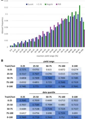
Having explored our models’ chemical feature learning, we lastly investigated the effect of reac-tion yield, as it is a critical feature of synthesis data. Unsurprisingly, plotting the distribution of reaction yields in each dataset showed a uni-formly strong bias towards high-yielding reac-tions (Figure 7A). Given the skewness of the data in this regard, we hypothesized that mod-els would perform best at predicting conditions for high-yielding reactions.

We divided the dataset into quartiles by re-action yield and re-trained the AR-GCN with each sub-set, subsequently testing in each region and on the full test set (Figure 7B). Intuitively, models trained in any yield range tended to give highest accuracy when tested in the same range, occupying the confusion matrix diagonal in Figure 7B (top). To our surprise, however, the standard model trained on the full dataset gave consistently high accuracies, regardless of the test set (bottom row).

Since the yield bins contain varying amounts of data, we re-split the dataset, again ordered by yield but with equal sub-set sizes (Figure 7B bot-tom). A similar trend was observed where the

Figure 7: Performance dependence on reaction yield. A) Distribution of reaction yields for the four datasets. B) AR-GCN average top-1 Ac

values for Suzuki predictions when trained and tested in different yield ranges (top) and dataset quartiles arranged by yield (bottom).

highest accuracies were found on the diagonal and bottom row of the confusion matrix. Inter-estingly, the worst performing model was that trained in the highest yield range and tested in the lowest. We recognize that making “inaccu-rate” predictions on low-yielding reactions offers an avenue for predictive reaction optimization and future studies will explore this objective.

4 Conclusion and Outlook

In summary, we present a multi-label classifica-tion approach to predicting experimental reac-tion condireac-tions for organic synthesis. We suc-cessfully model four high-value reaction types using expert-crafted label dictionaries: Suzuki, C–N, and Negishi couplings, and Pauson–Khand

(14)

reactions. We explore and optimize two model classes: gradient boosting machines and graph convolutional networks. We find that GCN mod-els perform very well in larger datasets, while GBMs show success for smaller datasets.

We report the first use of classifier trellises in molecular machine learning, and find that they are able to incorporate label correlations in modeling. We introduce a novel reaction-level graph attention mechanism that provides significant accuracy gains when coupled with relational GCNs, and construct a hybrid GCN architecture called attended relational GCNs, or AR-GCNs. We further provide an analytical framework for the chemical interpretation of our models, extracting the trellis structures and mutual information matrices of the CT-GBMs, and visualizing the attention weights assigned in AR-GCN predictions.

Experimental studies are currently underway assessing the feasibility of model predictions on novel reactions. Additionally, efforts to apply our modeling framework to less-structured re-action types such as oxidations and reductions are ongoing. Future studies will address the interplay between structure representation and classifier chaining, as well as the extension of our reaction attention mechanism to other tasks. We expect the work herein to be very informa-tive for future condition prediction studies, a highly valuable but underexplored learning task.

Acknowledgement We thank Prof Pietro

Perona for mentorship guidance and helpful project discussions, and Chase Blagden for help structuring the GBM experiments. Fellowship support was provided by the NSF (M.R.M., T.J.D Grant No. DGE- 1144469). S.E.R. is a Heritage Medical Research Institute Investiga-tor. Financial support from Research Corpora-tion is warmly acknowledged.

Supporting Information

Avail-able

This will usually read something like: “Exper-imental procedures and characterization data for all new compounds. The class will

automati-cally add a sentence pointing to the information on-line:

References

(1) Dreher, S. D. Catalysis in medicinal chem-istry. Reaction Chemistry & Engineering

2019, 4, 1530–1535.

(2) Blakemore, D. C.; Castro, L.; Churcher, I.;

Rees, D. C.; Thomas, A. W.;

Wil-son, D. M.; Wood, A. Organic synthesis provides opportunities to transform drug discovery.Nature Chemistry 2018,10, 383– 394.

(3) Mahatthananchai, J.; Dumas, A. M.; Bode, J. W. Catalytic Selective Synthesis.

Angewandte Chemie International Edition

2012, 51, 10954–10990.

(4) Reid, J. P.; Sigman, M. S. Comparing quan-titative prediction methods for the discov-ery of small-molecule chiral catalysts. Na-ture Reviews Chemistry 2018, 2, 290–305.

(5) Butler, K. T.; Davies, D. W.;

Cartwright, H.; Isayev, O.; Walsh, A. Machine learning for molecular and materials science. Nature 2018, 559, 547–555.

(6) Wu, Z.; Ramsundar, B.; Feinberg, E. N.; Gomes, J.; Geniesse, C.; Pappu, A. S.; Leswing, K.; Pande, V. MoleculeNet: a benchmark for molecular machine learning.

Chemical Science 2018, 9, 513–530. (7) Yang, K.; Swanson, K.; Jin, W.; Coley, C.;

Eiden, P.; Gao, H.; Guzman-Perez, A.; Hopper, T.; Kelley, B.; Mathea, M.; Palmer, A.; Settels, V.; Jaakkola, T.; Jensen, K.; Barzilay, R. Analyzing Learned Molecular Representations for Property Prediction. Journal of Chemical Informa-tion and Modeling 2019,59, 3370–3388. (8) Withnall, M.; Lindel¨of, E.; Engkvist, O.;

Chen, H. Building attention and edge mes-sage passing neural networks for bioactivity

(15)

and physical–chemical property prediction.

Journal of Cheminformatics 2020, 12.

(9) Stokes, J. M. et al. A Deep Learning Ap-proach to Antibiotic Discovery. Cell 2020,

180, 688–702.e13.

(10) Blaschke, T.; Olivecrona, M.; Engkvist, O.; Bajorath, J.; Chen, H. Application of Gen-erative Autoencoder in De Novo Molecular Design. Molecular Informatics 2018, 37, 1700123.

(11) Elton, D. C.; Boukouvalas, Z.; Fuge, M. D.; Chung, P. W. Deep learning for molecular design—a review of the state of the art.

Molecular Systems Design & Engineering

2019, 4, 828–849.

(12) Prykhodko, O.; Johansson, S. V.; Kot-sias, P.-C.; Ar´us-Pous, J.; Bjerrum, E. J.; Engkvist, O.; Chen, H. A de novo molec-ular generation method using latent vec-tor based generative adversarial network.

Journal of Cheminformatics 2019,11, 74. (13) Moret, M.; Friedrich, L.; Grisoni, F.; Merk, D.; Schneider, G. Generating Cus-tomized Compound Libraries for Drug Dis-covery with Machine Intelligence.2019, (14) Panteleev, J.; Gao, H.; Jia, L. Recent

ap-plications of machine learning in medicinal chemistry. Bioorganic & Medicinal Chem-istry Letters 2018,28, 2807–2815.

(15) Skoraczy´nski, G.; Dittwald, P.; Miasoje-dow, B.; Szymku´c, S.; Gajewska, E. P.; Grzybowski, B. A.; Gambin, A. Predict-ing the outcomes of organic reactions via machine learning: are current descriptors sufficient? Scientific Reports 2017, 7. (16) Coley, C. W.; Barzilay, R.; Jaakkola, T. S.;

Green, W. H.; Jensen, K. F. Prediction of Organic Reaction Outcomes Using Ma-chine Learning.ACS Central Science2017,

3, 434–443.

(17) Ahneman, D. T.; Estrada, J. G.; Lin, S.; Dreher, S. D.; Doyle, A. G. Predicting re-action performance in C–N cross-coupling

using machine learning.Science 2018,360, 186–190.

(18) Nielsen, M. K.; Ahneman, D. T.; Ri-era, O.; Doyle, A. G. Deoxyfluorination with Sulfonyl Fluorides: Navigating Reac-tion Space with Machine Learning.Journal of the American Chemical Society 2018,

140, 5004–5008.

(19) Sim´on-Vidal, L.; Garc´ıa-Calvo, O.;

Oteo, U.; Arrasate, S.; Lete, E.;

Sotomayor, N.; Gonz´alez-D´ıaz, H. Perturbation-Theory and Machine Learn-ing (PTML) Model for High-Throughput Screening of Parham Reactions: Experi-mental and Theoretical Studies. Journal of Chemical Information and Modeling

2018, 58, 1384–1396.

(20) Granda, J. M.; Donina, L.; Dragone, V.; Long, D.-L.; Cronin, L. Controlling an or-ganic synthesis robot with machine learn-ing to search for new reactivity. Nature

2018, 559, 377–381.

(21) Hughes, T. B.; Miller, G. P.; Swami-dass, S. J. Modeling Epoxidation of Drug-like Molecules with a Deep Machine Learn-ing Network. ACS Central Science 2015,

1, 168–180.

(22) Peng, Q.; Duarte, F.; Paton, R. S. Com-puting organic stereoselectivity – from con-cepts to quantitative calculations and pre-dictions. Chemical Society Reviews 2016,

45, 6093–6107.

(23) Banerjee, S.; Sreenithya, A.; Sunoj, R. B. Machine learning for predicting product distributions in catalytic regioselective reactions. Physical Chemistry Chemical Physics 2018, 20, 18311–18318.

(24) Beker, W.; Gajewska, E. P.; Badowski, T.; Grzybowski, B. A. Prediction of Major Regio-, Site-, and Diastereoisomers in Diels–Alder Reactions by Using Machine-Learning: The Importance of Physi-cally Meaningful Descriptors. Angewandte Chemie International Edition 2019, 58,

4515–4519. 14

(16)

(25) Zahrt, A. F.; Henle, J. J.; Rose, B. T.; Wang, Y.; Darrow, W. T.; Denmark, S. E. Prediction of higher-selectivity catalysts by computer-driven workflow and machine learning. Science 2019, 363, eaau5631. (26) Coley, C. W.; Green, W. H.; Jensen, K. F.

Machine Learning in Computer-Aided Syn-thesis Planning. Accounts of Chemical Re-search 2018,51, 1281–1289.

(27) Segler, M. H. S.; Preuss, M.; Waller, M. P. Planning chemical syntheses with deep neural networks and symbolic AI. Nature

2018, 555, 604–610.

(28) Coley, C. W.; Green, W. H.; Jensen, K. F. RDChiral: An RDKit Wrapper for Han-dling Stereochemistry in Retrosynthetic Template Extraction and Application.

Journal of Chemical Information and Mod-eling 2019, 59, 2529–2537.

(29) Badowski, T.; Gajewska, E. P.; Molga, K.; Grzybowski, B. A. Synergy Between Ex-pert and Machine-Learning Approaches Al-lows for Improved Retrosynthetic Planning.

Angewandte Chemie International Edition

2020, 59, 725–730.

(30) Nicolaou, C. A.; Watson, I. A.; LeMas-ters, M.; Masquelin, T.; Wang, J. Context Aware Data-Driven Retrosynthetic Analy-sis. Journal of Chemical Information and Modeling 2020,

(31) Gao, H.; Struble, T. J.; Coley, C. W.; Wang, Y.; Green, W. H.; Jensen, K. F. Us-ing Machine LearnUs-ing To Predict Suitable Conditions for Organic Reactions. ACS Central Science 2018,4, 1465–1476. (32) Ryou*, S.; Maser*, M. R.; Cui*, A. Y.;

DeLano, T. J.; Yue, Y.; Reisman, S. E. Graph Neural Networks for the Predic-tion of Substrate-Specific Organic Reac-tion CondiReac-tions.arXiv:2007.04275 [cs, LG]

2020,

(33) Huerta, F.; Hallinder, S.; Minidis, A.

Machine Learning to Reduce Reac-tion OptimizaReac-tion Lead Time – Proof

of Concept with Suzuki, Negishi and Buchwald-Hartwig Cross-Coupling Re-actions; preprint ChemRxiv.12613214, 2020.

(34) Schlichtkrull, M.; Kipf, T. N.; Bloem, P.; Berg, R. v. d.; Titov, I.; Welling, M. Mod-eling Relational Data with Graph Convo-lutional Networks. arXiv:1703.06103 [cs, stat] 2017,

(35) Friedman, J. H. Greedy Function Approx-imation: A Gradient Boosting Machine.

The Annals of Statistics 2001, 29, 1189– 1232.

(36) Reaxys. https://new.reaxys.com/, (ac-cessed on May 13, 2019).

(37) Weininger, D. SMILES, a chemical lan-guage and information system. 1. Introduc-tion to methodology and encoding rules.

Journal of Chemical Information and Mod-eling 1988, 28, 31–36.

(38) Cui, Y.; Jia, M.; Lin, T.-Y.; Song, Y.;

Belongie, S. Class-Balanced Loss

Based on Effective Number of Sam-ples. arXiv:1901.05555 [cs] 2019,

(39) Wu, X.-Z.; Zhou, Z.-H. A Unified View of Multi-Label Performance Measures.

arXiv:1609.00288 [cs] 2017,

(40) Natekin, A.; Knoll, A. Gradient boosting machines, a tutorial. Frontiers in Neuro-robotics 2013, 7.

(41) Ke, G.; Meng, Q.; Finley, T.; Wang, T.; Chen, W.; Ma, W.; Ye, Q.; Liu, T.-Y. In

Advances in Neural Information Process-ing Systems 30; Guyon, I., Luxburg, U. V., Bengio, S., Wallach, H., Fergus, R., Vish-wanathan, S., Garnett, R., Eds.; Curran Associates, Inc., 2017; pp 3146–3154. (42) Moriwaki, H.; Tian, Y.-S.; Kawashita, N.;

Takagi, T. Mordred: a molecular descrip-tor calculadescrip-tor.Journal of Cheminformatics

2018, 10, 4.

(43) Breiman, L. Random Forests. Machine Learning 2001, 45, 5–32.

(17)

(44) Zhang, M.-L.; Zhou, Z.-H. A Review on Multi-Label Learning Algorithms. IEEE Transactions on Knowledge and Data

En-gineering 2014, 26, 1819–1837.

(45) Read, J.; Pfahringer, B.; Holmes, G.; Frank, E. Classifier Chains for Multi-label Classification. Machine Learning and Knowledge Discovery in Databases. Berlin, Heidelberg, 2009; pp 254–269.

(46) Read, J.; Martino, L.; Olmos, P.; Lu-engo, D. Scalable Multi-Output Label Pre-diction: From Classifier Chains to Clas-sifier Trellises. Pattern Recognition 2015,

48, 2096–2109.

(47) Gilmer, J.; Schoenholz, S. S.; Riley, P. F.; Vinyals, O.; Dahl, G. E. Neural Mes-sage Passing for Quantum Chemistry.

arXiv:1704.01212 [cs] 2017,

(48) Veliˇckovi´c, P.; Cucurull, G.; Casanova, A.; Romero, A.; Li`o, P.; Bengio, Y. Graph Attention Networks. arXiv:1710.10903 [cs, stat] 2018,

(49) Busbridge, D.; Sherburn, D.; Cavallo, P.; Hammerla, N. Y. Relational Graph Atten-tion Networks. arXiv:1904.05811 [cs, stat]

2019,

(50) Tokui, S.; Oono, K.; Hido, S.; Clayton, J. Chainer: a Next-Generation Open Source Framework for Deep Learning. 2015, (51) Newman, M. E. J. Power laws, Pareto

dis-tributions and Zipf’s law. Contemporary Physics 2005, 46, 323–351.

(52) Zhou, K.; Dong, Y.; Lee, W. S.; Hooi, B.; Xu, H.; Feng, J. Effective Training Strate-gies for Deep Graph Neural Networks.

arXiv:2006.07107 [cs, stat] 2020,

(53) Galvez, J.; Garcia, R.; Salabert, M. T.; Soler, R. Charge Indexes. New Topological Descriptors. Journal of Chemical Informa-tion and Modeling 1994,34, 520–525.

(54) Moreau, G.; Broto, P. The Autocorrelation of a Topological Structure: A New Molecu-lar Descriptor. New Journal of Chemistry

1980,4, 359–360.

(55) Hollas, B. An Analysis of the Autocorrela-tion Descriptor for Molecules. Journal of Mathematical Chemistry 2003,33, 91–101.

(56) Chuang, K. V.; Keiser, M. J. Adversar-ial Controls for Scientific Machine Learn-ing.ACS Chemical Biology 2018,13, 2819– 2821.

(57) Landrum, G. A. RDKit: Open-Source Cheminformatics Software. (accessed Nov 20, 2016).

(18)

Graphical TOC Entry

(19)

download file view on ChemRxiv

(20)

Supporting Information:

Multi-Label Classification Models for the

Prediction of Cross-Coupling Reaction Conditions

Michael R. Maser,

†,§

Alexander Y. Cui,

‡,§

Serim Ryou,

¶,§

Travis J. DeLano,

†

Yisong Yue,

‡

and Sarah E. Reisman

∗,†

†Division of Chemistry and Chemical Engineering, California Institute of Technology, Pasadena, California, USA

‡Department of Computing and Mathematical Sciences, California Institute of Technology, Pasadena, California, USA

¶Computational Vision Lab, California Institute of Technology, Pasadena, California, USA §Equal contribution.

E-mail: [email protected]

S1

Data preparation and reaction dictionaries

Full procedures for data processing are outlined in our previous preprint.S1 An example protocol with full code is included in the associated github repository: https://github.com /slryou41/reaction-gcnn.git in the path: data/data processing example.ipynb. The worked example includes procedures for sorting reagents into categories by reaction role and aggregating into a full reaction dictionary. Final dictionaries for all four datasets as .csv files can be found in the repository path: data/all dictionaries/, and are tabulated below.

(21)

Table S1: Suzuki dataset dictionary.

category bin label dataset name instances

metal M1 tetrakis(triphenylphosphine) palladium(0) 55829 M2 palladium diacetate 16927 M3 (1,1’-bis(diphenylphosphino)ferrocene)palladium(II) dichloride 13723 M4 dichloro(1,1’-bis(diphenylphosphanyl)ferrocene)palladium(II)*CH2Cl2 8918 M5 bis-triphenylphosphine-palladium(II) chloride 8761 M6 tris-(dibenzylideneacetone)dipalladium(0) 5241 M7 palladium dichloride 1512 M8 bis(dibenzylideneacetone)-palladium(0) 1013 M9 dichloro[1,1’-bis(di-t-butylphosphino)ferrocene]palladium(II) 1074 M10 bis(tri-t-butylphosphine)palladium(0) 736 M11 chloro(2-dicyclohexylphosphino-2?,4?,6?- triisopropyl-1,1?-biphenyl)[2-(2?-amino-1,1?-biphenyl?)]palladium(II) 729 M12 bis(di-tert-?butyl(4-?dimethylaminophenyl)?phosphine)?dichloropalladium(II) 711 M13 bis(eta3-allyl-mu-chloropalladium(II)) 559 M14 tris(dibenzylideneacetone)dipalladium(0) chloroform complex 509

M15 palladium 10% on activated carbon 861

M16 sodium tetrachloropalladate(II) 283 M17 palladium 280 M18 (2-dicyclohexylphosphino-2?,4?,6?-triisopropyl- 1,1?-biphenyl)[2-(2?-amino-1,1?-biphenyl)]palladium(II) methanesulfonate 191 M19 bis(benzonitrile)palladium(II) dichloride 179 M20 (1,2-dimethoxyethane)dichloronickel(II) 158 M21 bis(1,5-cyclooctadiene)nickel (0) 155 M22 [1,3-bis(2,6-diisopropylphenyl)imidazol-2-ylidene](3-chloropyridyl)palladium(ll) dichloride 151 M23 (bis(tricyclohexyl)phosphine)palladium(II) dichloride 148 M24 dichloro bis(acetonitrile) palladium(II) 143

M25 Pd EnCat-30TM 137

M26 nickel(II) nitrate hexahydrate 106

M27 palladium(II) trifluoroacetate 106

Continued on next page

(22)

Table S1 – continued from previous page

M28 dichlorobis[1-(dicyclohexylphosphanyl)piperidine]palladium(II) 102 L1 triphenylphosphine 4489 L2 dicyclohexyl-(2’,6’-dimethoxybiphenyl-2-yl)-phosphane 3163 L3 XPhos 2100 L4 tricyclohexylphosphine 1808 L5 tris-(o-tolyl)phosphine 902 L6 tri-tert-butyl phosphine 694 L7 tri tert-butylphosphoniumtetrafluoroborate 616 L8 trisodium tris(3-sulfophenyl)phosphine 556 L9 1,1’-bis-(diphenylphosphino)ferrocene 486 ligand L10 4,5-bis(diphenylphos4,5-bis(diphenylphosphino)-9,9-dimethylxanthenephino)-9,9-dimethylxanthene 424 L11 CyJohnPhos 370 L12 ruphos 293 L13 1,3,5,7-tetramethyl-8-phenyl-2,4,6-trioxa-8-phosphatricyclo[3.3.1.13,7]decane 279 L14 tricyclohexylphosphine tetrafluoroborate 240 L15 johnphos 223 L16 4,4’-di-tert-butyl-2,2’-bipyridine 216 L17 catacxium A 192 L18 trifuran-2-yl-phosphane 183 L19 triphenyl-arsane 182 L20 1,1’-bis(di-tertbutylphosphino)ferrocene 142 L21 2,2’-bis-(diphenylphosphino)-1,1’-binaphthyl 129 L22 Tedicyp 218 L23 bis[2-(diphenylphosphino)phenyl] ether 108 B1 potassium carbonate 48981 B2 sodium carbonate 39769 B3 potassium phosphate 17799 B4 caesium carbonate 13345 B5 sodium hydrogencarbonate 3722 B6 cesium fluoride 2810 B7 sodium hydroxide 2156 B8 potassium hydroxide 2155 B9 potassium fluoride 2097 B10 triethylamine 1370

B11 potassium phosphate tribasic trihydrate 1016

B12 potassium acetate 931

B13 potassium tert-butylate 912

(23)

B14 potassium phosphate monohydrate 826

B15 sodium acetate 418

base B16 sodium t-butanolate 392

B17 barium dihydroxide 374

B18 N-ethyl-N,N-diisopropylamine 336

B19 lithium hydroxide 321

B20 potassium phosphate tribasic heptahydrate 317

B21 diisopropylamine 209

B22 sodium methylate 175

B23 tetrabutyl ammonium fluoride 173

B24 barium hydroxide octahydrate 171

B25 potassium dihydrogenphosphate 166

B26 potassium fluoride dihydrate 156

B27 1,4-diaza-bicyclo[2.2.2]octane 154

B28 lithium hydroxide monohydrate 143

B29 tetra-butylammonium acetate 137

B30 sodium phosphate 133

B31 potassium hydrogencarbonate 131

B32 dipotassium hydrogenphosphate 127

B33 tripotassium phosphate n hydrate 123

B34 cesiumhydroxide monohydrate 112

B35 sodium phosphate dodecahydrate 103

solvent S1 tetrahydrofuran 18113 S2 ethanol 24836 S3 methanol 4374 S4 1,4-dioxane 39107 S5 1,2-dimethoxyethane 19131 S6 acetonitrile 4366 S7 toluene 28304 S8 N,N-dimethyl formamide 15110 S9 water 92175 S10 1-methyl-pyrrolidin-2-one 472 additive A1 tetrabutylammomium bromide 3003 A2 water 1606 A3 lithium chloride 819 A4 hydrogenchloride 780 A5 copper(l) iodide 546 A6 silver(l) oxide 405 A7 copper diacetate 183 A8 dmap 181 A9 Aliquat 336 169

(24)

A10 cetyltrimethylammonim bromide 167

A11 copper(l) chloride 164

A12 potassium bromide 157

A13 trifluoroacetic acid 151

A14 oxygen 148

A15 air 112

A16 18-crown-6 ether 127

A17 sodium dodecyl-sulfate 113

Table S2: C–N dataset dictionary.

M1 copper(l) iodide 8180 M2 tris-(dibenzylideneacetone)dipalladium(0) 6995 M3 palladium diacetate 4668 M4 copper 1875 M5 bis(dibenzylideneacetone)-palladium(0) 1292 M6 copper(I) oxide 932 M7 copper(II) oxide 402 M8 copper(l) chloride 386 M9 copper(I) bromide 348 M10 bis(eta3-allyl-mu-chloropalladium(II)) 433

M11 copper(II) acetate monohydrate 352

M12 (1,1’-bis(diphenylphosphino)ferrocene)palladium(II) dichloride 159 M13 bis(tri-t-butylphosphine)palladium(0) 181 M14 iron(III) chloride 116 M15 copper(II) bis(trifluoromethanesulfonate) 91 M16 copper(ll) bromide 88 M17 bis-triphenylphosphine-palladium(II) chloride 82 M18 copper(II) sulfate 154 M19 bis(acetylacetonate)nickel(II) 78

M20 palladium 10% on activated carbon 71

M21 tetrakis(triphenylphosphine) palladium(0) 68 M22 dichlorobis(tri-O-tolylphosphine)palladium 67 M23 (1,2-dimethoxyethane)dichloronickel(II) 66

M24 palladium dichloride 63

M25 copper(I) thiophene-2-carboxylate 58

M26 cobalt(II) oxalate dihydrate 56

Continued on next page S-5

(25)

M27 copper dichloride 52 metal M28 dichloro(1,3-bis(2,6-bis(3- pentyl)phenyl)imidazolin-2-ylidene)(3-chloropyridyl)palladium(II) 49 M29 chloro[2-(dicyclohexylphosphino)-3

,6-dimethoxy-2?,4?, 6?-triisopropyl- 1,1?-biphenyl] [2-(2-aminoethyl)phenyl]palladium(II) 97 M30 [2-(di-tert-butylphosphino)-2?,4?,6?-triisopropyl- 1,1?-biphenyl][2-((2-aminoethyl)phenyl)]palladium(II) chloride 49 M31 iron(III) oxide 48 M32 C36H45Cl2N3OPd 46

M33 nickel(II) bromide trihydrate 45

M34 copper acetylacetonate 45 M35 C36H43Cl2N3Pd 45 M36 C30H43O2P*C13H12N(1-)*CH3O3S(1-)*Pd(2+) 45 M37 bis(1,5-cyclooctadiene)nickel (0) 45 M38 CuPy2Cl2 42 M39 dichloro(3-chloropyridinyl)(1,3- (diisopropylphenyl)-4,5- bis(dimethylamino)imidazol-2-ylidene)palladium(II) 41 M40 Al2O3*Cu(2+) 40 M41 C33H40ClN3O2Pd 38 M42 dichloro(1,1’-bis(diphenylphosphanyl)ferrocene)palladium(II)*CH2Cl2 36 M43 (1,3-bis(2,6-diisopropylphenyl)-3,4,5,6-tetrahydropyrimidin-2-ylidene)Pd(cinnamyl, 3-phenylallyl)Cl 36 M44 copper(II)iodide 35 L1 2,2’-bis-(diphenylphosphino)-1,1’-binaphthyl 3014 L2 tri-tert-butyl phosphine 2137 L3 4,5-bis(diphenylphos4,5-bis(diphenylphosphino)-9,9-dimethylxanthenephino)-9,9-dimethylxanthene 1995 L4 N,N‘-dimethylethylenediamine 1543 L5 XPhos 830 L6 1,10-Phenanthroline 703 L7 L-proline 620 L8 1,1’-bis-(diphenylphosphino)ferrocene 653 L9 johnphos 444 L10 DavePhos 374

(26)

L11 triphenylphosphine 275 L12 ruphos 266 L13 tri tert-butylphosphoniumtetrafluoroborate 265 L14 tert-butyl XPhos 242 L15 dicyclohexyl-(2’,6’-dimethoxybiphenyl-2-yl)-phosphane 261 L16 trans-1,2-Diaminocyclohexane 724 L17 8-quinolinol 206 L18 CyJohnPhos 192 L19 trans-N,N’-dimethylcyclohexane-1,2-diamine 535 L20 ethylenediamine 175 L21 dimethylaminoacetic acid 167 L22 dicyclohexyl[3,6-dimethoxy-2?,4?,6?-tris(1-methylethyl)[1,1?-biphenyl]-2-yl]phosphine 165 L23 2,2,6,6-tetramethylheptane-3,5-dione 163 L24 1,1’-bi-2-naphthol 162 L25 bis[2-(diphenylphosphino)phenyl] ether 170 L26 1-dicyclohexylphosphino-2-di-tert-butylphosphinoethylferrocene 142 ligand L27 P(i-BuNCH2)3CMe 110 L28 di-tert-butyl2?-isopropoxy-[1,1?-binaphthalen]-2-ylphosphane 108 L29 di-tert-butyl(2,2-diphenyl-1-methyl-1-cyclopropyl)phosphine 104 L30 P(i-BuNCH2CH2)3N 98 L31 N,N-dimethylglycine hydrochoride 96 L32 N-[2-(di(1-adamantyl)phosphino)phenyl]morpholine 92 L33 5-(di-tert-butylphosphino)-1?, 3?, 5?-triphenyl-1?H-[1,4?]bipyrazole 91 L34 2-[2-(dicyclohexylphosphino)-phenyl]-1-methyl-1H-indole 86 L35 4,4’-di-tert-butyl-2,2’-bipyridine 85 L36 tris-(o-tolyl)phosphine 77 L37 2,8,9-tris(2-methylpropyl)-2,5,8,9-tetraaza-1-phosphabicyclo[3.3.3]undecane 75 L38 cis-N,N’-dimethyl-1,2-diaminocyclohexane 74 L39 monophosphine 1,2,3,4,5-pentaphenyl-1’-(di-tert-butylphosphino)ferrocene 55 L40 5-(di(adamantan-1-yl)phosphino)-1?,3?,5?-triphenyl-1?H-1,4?-bipyrazole 55 L41 t-BuBrettPhos 53

(27)

L42 2-(N,N-dimethylamino)athanol 53 L43 tricyclohexylphosphine 46 L44 (E)-3-(dimethylamino)-1-(2-hydroxyphenyl)prop-2-en-1-one 46 L45 di-tert-butylneopentylphosphonium tetrafluoroborate 38 L46 2-di-tertbutylphosphino-3,4,5,6-tetramethyl-2’,4’,6’-triisopropyl-1,1’-biphenyl 37 L47 N,N,N,N,-tetramethylethylenediamine 26 base B1 sodium t-butanolate 9103 B2 potassium carbonate 7129 B3 caesium carbonate 6957 B4 potassium phosphate 3274 B5 potassium tert-butylate 2167 B6 potassium hydroxide 1420 B7 triethylamine 500 B8 lithium hexamethyldisilazane 432 B9 sodium hydroxide 430 B10 sodium hydride 228 B11 sodium carbonate 200

B12 potassium phosphate monohydrate 130

B13 sodium hydrogencarbonate 128 solvent S1 toluene 11970 S2 1,4-dioxane 5273 S3 N,N-dimethyl-formamide 4246 S4 dimethyl sulfoxide 3790 S5 water 2464 S6 tetrahydrofuran 1457 S7 1,2-dimethoxyethane 878 S8 tert-butyl alcohol 841 S9 acetonitrile 780 S10 ethanol 549 S11 5,5-dimethyl-1,3-cyclohexadiene 497 S12 isopropyl alcohol 316 S13 nitrobenzene 315 S14 1-methyl-pyrrolidin-2-one 292 S15 hexane 286 S16 N,N-dimethyl acetamide 281 S17 1,2-dichloro-benzene 254

S18 neat (no solvent) 240

S19 o-xylene 219

(28)

S20 xylene 208 S21 methanol 180 S22 ethyl acetate 163 A1 18-crown-6 ether 455 A2 tetrabutylammomium bromide 372 A3 8-quinolinol 206 A4 dimethylaminoacetic acid 167 A5 1,1’-bi-2-naphthol 162 A6 water 160 A7 sodium sulfate 132 A8 2-(2-methyl-1-oxopropyl)cyclohexanone 121 A9 phenylboronic acid 120 A10 1,3-bis[(2,6-diisopropyl)phenyl]imidazolinium chloride 109

A11 potassium iodide 108

A12 hydrogenchloride 107

A13 ethylene glycol 102

A14 N,N-dimethylglycine hydrochoride 96

A15 1,3-bis[2,6-diisopropylphenyl]imidazolium chloride 95

A16 N-ethylmorpholine 93

A17 tert-butyl alcohol 87

A18 aluminum oxide 84

A19 D-glucose 83

A20 cetyltrimethylammonim bromide 71

A21 1,3-dimethyl-3,4,5,6-tetrahydro-2(1H)-pyrimidinone

68 A22 N’,N’-diphenyl-1H-pyrrole-2-carbohydrazide 63

A23 manganese(II) fluoride 63

A24 dimethyl sulfoxide 55

A25 2-(N,N-dimethylamino)athanol 53

A26 air 48

A27 iron(III) oxide 48

A28 (E)-3-(dimethylamino)-1-(2-hydroxyphenyl)prop-2-en-1-one

46

A29 lithium bromide 44

A30 6,7-dihydro-5H-quinolin-8-one oxime 43

A31 CVT-2537 42

A32 ammonium chloride 42

A33 1-methyl-pyrrolidin-2-one 42

A34 tetra(n-butyl)ammonium hydroxide 40

A35 salicylaldehyde-oxime 39

A36 potassium fluoride on basic alumina 39

(29)

additive

A37 toluene-4-sulfonic acid 38

A38 lithium chloride 38

A39 pipecolic Acid 37

A40 oxygen 37

A41 metformin hydrochloride 37

A42 8-Hydroxyquinoline-N-oxide 37

A43 1-(5,6,7,8-tetrahydroquinolin-8-yl)ethan-1-one 36

A44 tetrabutyl ammonium fluoride 36

A45 N1,N2-bis(thiophen-2-ylmethyl)oxalamide 36 A46 N-phenyl-2-pyridincarboxamide-1-oxide 35 A47 N-((1-oxy-pyridin-2-yl)methyl)oxalamic acid 35

A48 C19H19N5O 35

A49 manganese(II) chloride tetrahydrate 34

A50 1-tetralone oxime 32

A51 N1,N2-bis(2,4,6-trimethoxyphenyl)oxalamide 31

A52 N-methoxy-1H-pyrrole-2-carboxamide 29

A53 ammonia 29

A54 1,2,3-Benzotriazole 29

A55 dimethylenecyclourethane 28

A56 isopropylmagnesium chloride 27

A57 N-(2-cyanophenyl)pyridine-2-carboxamide 27

A58 C20H18N2O2 27

A59 2-acetylcyclohexanone 27

A60 2,6-di-tert-butyl-4-methyl-phenol 26

A61 2-hydroxy-pyridine N-oxide 26

A62 TPGS-750-M 25

A63 N?-phenyl-1H-pyrrole-2-carbohydrazide 25

A64 lanthanum(III) oxide 25

A65 ethylmagnesium bromide 25

A66 ethyl 2-oxocyclohexane carboxylate 25

A67 1,4-dimethyl-1,2,3,4-tetrahydro-5H-benzo[e][1,4]diazepin-5-one

25

A68 tetraethoxy orthosilicate 24

A69 N,N,N’,N’-tetramethylguanidine 24

A70 C20H26N4O4 24

A71 2-methyl-8-quinolinol 24

A72 2-carbomethoxy-3-hydroxyquinoxaline-di-N-oxide 24 A73 1,3-diisopropyl-1H-imidazol-3-ium chloride 24

A74 MOF-199 24

(30)

Table S3: Negishi dataset dictionary.

M1 tetrakis(triphenylphosphine) palladium(0) 1902 M2 tris-(dibenzylideneacetone)dipalladium(0) 572 M3 bis-triphenylphosphine-palladium(II) chloride 418 M4 palladium diacetate 370 M5 bis(dibenzylideneacetone)-palladium(0) 344 M6 (1,1’-bis(diphenylphosphino)ferrocene)palladium(II) dichloride 334 M7 bis(tri-t-butylphosphine)palladium(0) 273 M8 dichloro(1,1’-bis(diphenylphosphanyl)ferrocene)palladium(II)*CH2Cl2 248 M9 dichlorobis[1-(dicyclohexylphosphanyl)piperidine]palladium(II) 168 M10 palladium(l) tri-tert-butylphosphine iodide dimer 101 M11 bis(tricyclohexylphosphine)nickel(II) dichloride 99 M12 [(C10H13-1,3-(CH2P(C6H11)2)2)Pd(Cl)] 87 M13 1,3-bis[(diphenylphosphino)propane]dichloronickel(II) 63 M14 bis(1,5-cyclooctadiene)nickel (0) 56 metal M15 nickel dichloride 56 M16 tris(dibenzylideneacetone)dipalladium(0) chloroform complex 46 M17 dichlorobis(tri-O-tolylphosphine)palladium 46 M18 palladium 44 M19 [1,3-bis(2,6-diisopropylphenyl)imidazol-2-ylidene](3chloro-pyridyl)palladium(II) dichloride 136 M20 C20H20ClN3Ni 42 M21 dichloro(1,3-bis(2,6-bis(3- pentyl)phenyl)imidazolin-2-ylidene)(3-chloropyridyl)palladium(II) 39 M22 bis(triphenylphosphine)nickel(II) chloride 38 M23 C26H24ClN2NiP*0.1C7H8 35 M24 cobalt(II) chloride 34 M25 copper(I) bromide 31 M26 C40H55Cl5N3Pd 30 M27 [1,3-bis(2,6-diisoheptylphenyl)-4,5- dichloroimidazol-2-ylidene](3-chloropyridyl)palladium(II) dichloride 29

M28 dichloro bis(acetonitrile) palladium(II) 29

(31)

M29 palladium(II) trifluoroacetate 27 M30 1,2-bis(diphenylphosphino)ethane nickel(II) chloride 27 M31 C27H22Cl2N3NiP 24 M32 C38H34Br2N4Ni2P2 23 L1 1,1’-bis-(diphenylphosphino)ferrocene 233 L2 dicyclohexyl-(2’,6’-dimethoxybiphenyl-2-yl)-phosphane 196 L3 XPhos 187 L4 triphenylphosphine 161 L5 trifuran-2-yl-phosphane 128 L6 monophosphine 1,2,3,4,5-pentaphenyl-1’-(di-tert-butylphosphino)ferrocene 95 L7 tris-(o-tolyl)phosphine 70 ligand L8 Ruphos 61 L9 2?-(dicyclohexylphophanyl)-N2,N2,N6,N6-tetramethyl[1,1?-biphenyl]-2,6-diamine 37 L10 tripiperidino-phosphine 37 L11 tri tert-butylphosphoniumtetrafluoroborate 35 L12 1,2-bis-(dicyclohexylphosphino)ethane 33 L13 4,5-bis(diphenylphos4,5-bis(diphenylphosphino)-9,9-dimethylxanthenephino)-9,9-dimethylxanthene 31 L14 N,N,N,N,-tetramethylethylenediamine 24 L15 [2,2]bipyridinyl 22 L16 4,4’-di-tert-butyl-2,2’-bipyridine 21 L17 1,2-Ph2-3,4-bis(2,4,6-(t-Bu)3-phenylphophinidene)cyclobutene 20 L18 johnphos 20 L19 tri-tert-butyl phosphine 19 L20 tricyclohexylphosphine 18 temperature T1 -163 - 18 101 T2 18 - 23 2313 T3 23 - 50 643 T4 50 - 61 975 T5 61 - 80 658 T6 80 - 100 673 T7 100 - 120 696 T8 120 - 220 479 S1 tetrahydrofuran 4525 S2 N,N-dimethyl-formamide 1003 S3 1-methyl-pyrrolidin-2-one 674

(32)

solvent S4 toluene 541 S5 1,4-dioxane 335 S6 N,N-dimethyl acetamide 247 S7 hexane 219 S8 diethyl ether 203 S9 water 122 S10 1,2-dimethoxyethane 67 additive A1 lithium chloride 243 A2 zinc 207 A3 copper(l) iodide 154 A4 water 62 A5 diisobutylaluminium hydride 59 A6 tetrabutylammomium bromide 52 A7 ammonium chloride 51 A8 n-butyllithium 46 A9 1-Methylpyrrolidine 42 A10 Li2CoCl4 42

A11 sodium formate 42

A12 hydrogenchloride 36

A13 caesium carbonate 36

A14 zinc diacetate 32

A15 potassium carbonate 30

A16 norborn-2-ene 30

A17 lithium bromide 28

A18 1,3-dimethyl-3,4,5,6-tetrahydro-2(1H)-pyrimidinone

23

A19 methylzinc chloride 22

A20 1-methyl-pyrrolidin-2-one 21

A21 zinc(II) chloride 21

A22 isoquinoline 20

A23 sodium carbonate 19

A24 1-ethyl-2-pyrrolidinone 18

A25 sodium 16

A26 1-methyl-1H-imidazole 15

A27 oxovanadium(V) ethoxydichloride 12

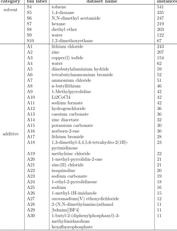
A28 2-(N,N-dimethylamino)athanol 11 A29 [bdmim][BF4] 11 A30 1-butyl-2-(diphenylphosphanyl)-3-methylimidazolium hexafluorophosphate 11 S-13

(33)

Table S4: PKR dataset dictionary.

M1 dicobalt octacarbonyl 614 M2 di(rhodium)tetracarbonyl dichloride 333 M3 chloro(1,5-cyclooctadiene)rhodium(I) dimer 140 M4 [RhCl(CO)dppp]2 92 M5 cobalt(II) bromide 44 M6 palladium dichloride 33 metal M7 dodecacarbonyl-triangulo-triruthenium 32 M8 Co2Rh2 nanoparticles immobilized on charcoal 50

M9 tetracobaltdodecacarbonyl 44

M10 molybdenum hexacarbonyl 23

M11 Rh(dppp)2Cl 19

M12 cobalt nanoparticles on charcoal 36

M13 methylidynetricobalt nonacarbonyl 25 M14 bis(triphenylphosphine)(carbonyl)rhodium chloride 11 M15 PdCl(OHNCCH3C6H4)(C5H5N) 10 M16 bis(1,5-cyclooctadiene)diiridium(I) dichloride 9 M17 diiron nonacarbonyl 9 M18 iron(II) bis(trimethylsilyl)amide 9 ligand L1 1,1,3,3-tetramethyl-2-thiourea 128 L2 1,3-bis-(diphenylphosphino)propane 93 L3 2,2’-bis-(diphenylphosphino)-1,1’-binaphthyl 31 L4 triphenylphosphine 16 L5 tri-n-butylphosphine sulfide 15 L6 (S)-3,5-di-tert-butyl-4-methoxyphenyl-(6,6?- dimethoxybiphenyl-2,2?-diyl)-bis(diphenylphosphine) 12 temperature T1 -98 - 20 83 T2 20 961 T3 20 - 60 299 T4 60 - 77 370 T5 77 - 94 338 T6 94 - 120 395 T7 120 - 180 303 S1 toluene 966 S2 dichloromethane 601 S3 tetrahydrofuran 318 S4 1,2-dichloro-ethane 171 S5 1,2-dimethoxyethane 145 S6 acetonitrile 141 S7 not listed 102

(34)

solvent S8 water 71 S9 benzene 76 S10 para-xylene 136 S11 hexane 43 S12 dimethyl sulfoxide 39 S13 1,4-dioxane 33 S14 dibutyl ether 33 S15 diethyl ether 22 activator A1 4-methylmorpholine N-oxide 420 A2 trimethylamine-N-oxide 212 A3 dimethyl sulfoxide 137 A4 cyclohexylamine 68

A5 n-butyl methyl sulfide 27

A6 silver trifluoromethanesulfonate 23

A7 silver tetrafluoroborate 18

A8 silver hexafluoroantimonate 19

A9 (4-fluorobenzyl)(methyl)sulfide 14

A10 dinitrogen monoxide 14

A11 4-methylmorpholine 4-oxide monohydrate 13

CO (g) G1 carbon monoxide 1169 G2 none 1580 additive O1 4 A molecular sieve 84 O2 zinc 50 O3 hydrogen 40 O4 ethylene glycol 30 O5 cetyltrimethylammonim bromide 22 O6 Celite 17 O7 Triton X(R)-100 37 O8 acetic anhydride 15 O9 lithium chloride 15 O10 water 11 O11 oxygen 10

O12 potassium carbonate 8

O13 triethylsilane 8 pressure P1 37 - 760 35 P2 760 2392 P3 760 - 7600 169 P4 7600 - 7500600 153 S-15

(35)

S2

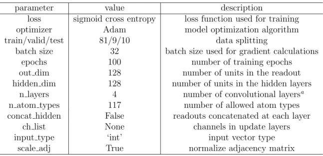
Computational details and hyperparameters

S2.1

Gradient-boosting machines (GBMs)

Numerical inputs for GBM models were constructed by tokenizing SMILES strings for each molecule in a reaction with character–to–number mappings, and calculating chemical descriptor vectors using Mordred.S2 _{Code examples for these processing protocols are provided}

in the associated github repository at the path data/gbm{ }inputs/parsing-cols.ipynb. All GBM classifiers were implemented using Microsoft’s lightGBM.S3 Specific non-default parameter settings are included in Table S5.

Table S5: Computational details and general parameters used for GBM models.

parameter value description

train/valid/test 81/9/10 data splittinga

max depth 7 maximum tree depth for base learners tree method ‘gpu hist’ split continuous features into discrete bins

eval metric ‘aucpr’ evaluation metric

a _{Training, validation, and test sets were identical to those in GCNs.}

S2.1.1 Binary relevance method (BM)

In BM experiments, an independent lightgbm.LGBMClassifier was fit for each label bin in a dataset’s dictionary using the full input representation.

S2.1.2 Classifier trellises (CTs)

In CT experiments, lightgbm.LGBMClassifiers were fit for each label bin in a dataset’s dictionary as part of a grid structure in which predictions are made sequentially and are passed to downstream models as additional inputs (see main text for explanation). Mutual information (MI) matrices were constructed for each dataset’s label dictionary using sci-kit learn’s sklearn.metrics.mutual info score module.S4 Classifier trellises were then constructed following the algorithm reported by Read et al. (see main text and associated code for details).S5 As shown in the example in the main text, each model takes additional