NSUWorks
CEC Theses and Dissertations College of Engineering and Computing2018
Machine Learning Methods for Septic Shock
Prediction
Aiman A. Darwiche
Nova Southeastern University,[email protected]
This document is a product of extensive research conducted at the Nova Southeastern UniversityCollege of Engineering and Computing. For more information on research and degree programs at the NSU College of Engineering and Computing, please clickhere.
Follow this and additional works at:https://nsuworks.nova.edu/gscis_etd
Part of theComputer Sciences Commons
Share Feedback About This Item
This Dissertation is brought to you by the College of Engineering and Computing at NSUWorks. It has been accepted for inclusion in CEC Theses and Dissertations by an authorized administrator of NSUWorks. For more information, please [email protected].
NSUWorks Citation
Aiman A. Darwiche. 2018.Machine Learning Methods for Septic Shock Prediction.Doctoral dissertation. Nova Southeastern University. Retrieved from NSUWorks, College of Engineering and Computing. (1051)
Machine Learning Methods for Septic Shock Prediction
by
Aiman A. Darwiche
A dissertation submitted in partial fulfillment of the requirements for the degree of Doctor of Philosophy
in
Computer Science
College of Engineering and Computing Nova Southeastern University
iii
An Abstract of a Dissertation Submitted to Nova Southeastern University in Partial Fulfillment of the Requirements for the Degree of Doctor of Philosophy
Machine Learning Methods for Septic Shock Prediction by
Aiman A. Darwiche July 2018
Sepsis is an organ dysfunction life-threatening disease that is caused by a dysregulated body response to infection. Sepsis is difficult to detect at an early stage, and when not detected early, is difficult to treat and results in high mortality rates. Developing improved methods for identifying patients in high risk of suffering septic shock has been the focus of much research in recent years. Building on this body of literature, this dissertation develops an improved method for septic shock prediction. Using the data from the MMIC-III database, an ensemble classifier is trained to identify high-risk patients. A robust prediction model is built by obtaining a risk score from fitting the Cox Hazard model on multiple input features. The score is added to the list of features and the Random Forest ensemble classifier is trained to produce the model. The Cox Enhanced Random Forest (CERF) proposed method is evaluated by comparing its predictive accuracy to those of extant methods.
Keywords: Sepsis, Septic Shock, Machine Learning, Prediction, Predictive Model, Classification, Ensemble Classifier
iv
Acknowledgements
When I decided to pursue a Ph.D. in Computer Science, I predicted, without applying any machine learning techniques, that the journey was going to be rough, challenging, but at the same time fulfilling. The mere fact that I started pursuing this goal while maintaining a full-time job as a software developer, meant that the road to success would be an upward battle that required extra efforts, sleepless nights, and sacrifices from all family members. For that, I would like to express my deepest thanks to my wife and kids, my parents, my brother and my sisters, and my sister-in-law for their continued support and patience throughout the whole adventure.
The utmost thanks go to my advisor Dr. Sumitra Mukherjee for his tremendous support and guidance from the day we set out together. His wisdom and knowledge provided the much-needed light to maneuver through the turbulences of the challenging PhD river. I would like also to thank Dr. Michael Laszlo and Dr.Francisco Mitropoulos, the dissertation committee members, who provided precious input that incredibly
v
Table of Contents Abstract iii
Acknowledgments iv List of Tables vii List of Figures ix Chapters 1. Introduction 1 Background 1 Problem Statement 3 Goal 3 Research Question 4
Relevance and Significance 4 Issues 5
Definition of Terms 6 Summary 7
2. Literature Review 8 Introduction 8
Septic Shock Prediction 8 Ensemble Classifiers 12
Types of ensemble classifiers 13 Combining methods 14
Ensemble Classifier Usage in the Medical Field 16 Cox Proportional Hazards Model 17
Random Forest 19
Septic Shock Biomarkers 21
3. Methodology 25
Specific Research Method Employed 25 1. Data Collection 25
2. Features Selection 28
3. Data Cleanup and Preparation 32 4. Prediction Model 35
Summary 42 4. Results 44 Overview 44 Model Results 44
1. Temperature, HR, RR, MAP, and SI Model 45
vi
3. Temperature, RR, Creatinine, Lactate, and WBC Model 47 4. Temperature, HR, Creatinine, Lactate, and WBC Model 48 5. HR, RR, MAP, SBP, and DBP Model 49
6. Temperature, HR, RR, SBP, DBP, SpO2, and GCS Model 49 7. DBP and Albumin Model 50
8. MSI Model 51
9. ageSI, Age, SBP, and Gender Model 52 Selected Model 53
Model Validation 54 Model Comparison 55 Summary 56
5. Conclusions, Implications, Recommendations, and Summary 57 Overview 57 Conclusions 57 Implications 59 Recommendations 60 Summary 61 References 63
vii List of Tables
Tables
1. Features that may feed into classifiers 28 2. Additional Researched Biomarkers 30
3. Final Features that were used feed into classifiers 32 4. Time Dependent Data Set Sample 34
5. Partitioned Data Sets Detailed Counts (patients with multiple admissions) 35 6. Time Dependent Data Set Sample at Time t=20 39
7. Cox Score Calculation Sample 39 8. Confusion Matrix 42
9. Summary of total count of patients, and counts in each class for all models 45 10. Temperature, HR, RR, MAP, and SI Model Coefficients 45
11. Temperature, HR, RR, MAP, and SI Model Confusion Matrix 46 12. Metrics for Temperature, HR, RR, MAP, and SI Model 46
13. Temperature, RR, MAP, Lactate, and WBC Model Coefficients 46 14. Temperature, RR, MAP, Lactate, and WBC Model Confusion Matrix 47 15. Metrics for Temperature, RR, MAP, Lactate, and WBC Model 47 16. Temperature, RR, Creatinine, Lactate, and WBC Model Coefficients 47 17. Temperature, RR, Creatinine, Lactate, and WBC Model Confusion Matrix 47 18. Metrics for Temperature, RR, Creatinine, Lactate, and WBC Model 48 19. Temperature, HR, Creatinine, Lactate, and WBC Model Coefficients 48 20. Temperature, HR, Creatinine, Lactate, and WBC Model Confusion Matrix 48
viii
21. Metrics for Temperature, HR, Creatinine, Lactate, and WBC Model 48 22. HR, RR, MAP, SBP, and DBP Model Coefficients 49
23. HR, RR, MAP, SBP, and DBP Model Confusion Matrix 49 24. Metrics for HR, RR, MAP, SBP, and DBP Model 49
25. Temperature, HR, RR, SBP, DBP, SpO2, and GCS Model Coefficients 50 26. Temperature, HR, RR, SBP, DBP, SpO2, and GCS Model Confusion Matrix 50 27. Metrics for Temperature, HR, RR, SBP, DBP, SpO2, and GCS Model 50 28. DBP and Albumin Model Coefficients 50
29. DBP and Albumin Model Confusion Matrix 51 30. Metrics for DBP and Albumin Model 51 31. MSI Model Coefficients 51
32. MSI Model Confusion Matrix 51 33. Metrics for MSI Model 52
34. ageSI, Age, SBP, and Gender Model Coefficients 52 35. ageSI, Age, SBP, and Gender Model Confusion Matrix 52 36. Metrics for ageSI, Age, SBP, and Gender Model 52 37. Cross Validation Results 55
ix
List of Figures
Figures
1. Patients Selection Criteria 27
2. Cox Model for Temperature, RR, MAP, lactate, and WBC 53 3. Temperature, RR, MAP, lactate, and WBC Model Results 55
Chapter 1
Introduction
Background
Sepsis is an ancient syndrome that has eluded medical practitioners throughout history (Martin, 2012). Hippocrates (460 BC - 370 BC), the Greek physician, talked about rotting flesh and festering wounds as signs of sepsis (Angus & van der Poll, 2013). At a later time, Marcus Terentius Varro, the Roman scholar and writer (116 BC – 27 BC) talked about tiny and invisible airborne creatures that caused dangerous diseases when inhaled (Martin, 2012). Niccolo Machiavelli (1469 – 1527), the Renaissance historian and philosopher, wrote in 1513 about a frenetic fever that was difficult to detect but easy to treat, whereas it would become very difficult to treat but easy to identify at a later stage (Martin, 2012). These syndromes closely matched sepsis (Martin, 2012). With Pasteur and others confirming the germ theory, sepsis was redefined as a systemic infection of the body by pathogenic organisms (germs) that spread in the bloodstream (Angus & van der Poll, 2013). However, despite successfully ridding the body of the invading
pathogens, lots of patients did not survive, which led researchers to believe that the body drove the pathogenesis of sepsis not the germs (Angus & van der Poll, 2013). In 1992, the American College of Chest Physicians (ACCP) and the Society of Critical Care Medicine (SCCM) jointly published a consensus definition of sepsis. Sepsis is a systemic inflammatory response of the body due to a microbial infection (King, Bauzá, Mella, &
Remick, 2014; Martin, 2012; Prucha, Bellingan, & Zazula, 2015). This definition remained in effect until 2016, when The Third International Consensus Definitions for Sepsis and Septic Shock (Sepsis-3) redefined sepsis as a “life-threatening organ
dysfunction caused by a dysregulated host response to infection” (Singer, Deutschman, Seymour, & et al., 2016). In addition, the group of experts of The Third International Consensus found that sepsis and severe sepsis were used interchangeably, thus they eliminated the use of severe sepsis and reclassified the progress of the disease as sepsis that could lead to septic shock (Singer et al., 2016). For the sake of this dissertation, we used both sepsis and severe sepsis diagnosis as they are part of the dataset utilized in this study.
Sepsis is a major worldwide health issue, which leads to death when it progresses to severe sepsis or septic shock (Deepak & Bhat, 2014; Henry, Hager, Pronovost, & Saria, 2015; Marty et al., 2013; Prucha et al., 2015). In the past twenty years, the
occurrence of sepsis is increasing not only in developing countries but in Western Europe and the United States as well (Prucha et al., 2015). In the United States, severe sepsis and septic shock will affect 750,000 patients every year resulting in 30% mortality and $15.4 billion in yearly heath care expenditures (Henry et al., 2015; Lausevic & Lausevic, 2012; Lukaszewski et al., 2008; Nguyen et al., 2014).
Medical professionals and researchers have tried early goal-directed therapy to decrease the percentage of deaths in patients suffering from severe sepsis and septic shock (Thiel et al., 2010). They explored timely interventions that involved fluid resuscitation and appropriate antibiotic administration, which proved to optimize the outcomes and reduce mortality (Nguyen et al., 2014; Sawyer et al., 2011).
Despite the progress that has been achieved in the past ten years to detect septic shock early, and despite the advancements in treatment that resulted in reducing
mortality, the percentage still remains high (Mohan, Shrestha, Guleria, Pandey, & Wig, 2015; Prucha et al., 2015). The need to implement a system that can identify patients with high risk of septic shock is very crucial (Sawyer et al., 2011). In fact, methods that can identify patients who will experience septic shock in the near future can help improve the outcome (Henry et al., 2015).
Problem Statement
The high mortality rate of sepsis is a major problem that faces the medical and research communities (Deepak & Bhat, 2014; Henry et al., 2015; Lausevic & Lausevic, 2012; Marty et al., 2013; Nguyen et al., 2014; Prucha et al., 2015). Identifying septic shock in a timely manner before it happens is crucial in reducing the mortality rate (Henry et al., 2015; Sawyer et al., 2011).
The septic shock prediction problem was modeled as a binary classification task: patients were classified into two groups – those who were at high risk of suffering a Septic Shock and those who were not – based on information available from clinical observations and laboratory test results. The solution was to train an ensemble classifier on available data and to implement a predictive model for this classification task. Goal
The study used the extensive data available from the MIMIC-III database to develop a model to predict septic shock. This work explored the ability of the model to increase the accuracy of septic shock prediction before its onset within a certain
computer-assisted decision support in the intensive care unit (ICU), which could allow medical professionals to reduce mortality among sepsis patients.
To support the goal, the dissertation considered the performance of the predictive model at detecting the patients who might have developed septic shock before its onset. First, a cross-validation technique was used to measure accuracy, sensitivity, and
specificity (Alberg, Park, Hager, Brock, & Diener-West, 2004; Simon, Subramanian, Li, & Menezes, 2011). An iterative k-fold cross-validation technique, with k=10 was used (Beleites, Neugebauer, Bocklitz, Krafft, & Popp, 2013; Refaeilzadeh, Tang, & Liu, 2009). Next, the performance of the model was compared to two different models. The first one was a routine screening protocol for septic shock that uses SIRS criteria,
suspicion of infection, and the presence of either hypotension or hyperlactatemia (Henry et al., 2015). The second evaluation was against the TREWScore model – a leading machine learning model developed by Henry et al. (2015).
Research Question
As mentioned, the goal of this study was to develop a model to predict septic shock using ensemble classification. Ensemble classification is known to increase accuracy; thus, the following research question guided the study:
RQ
How can one develop an ensemble model to predict septic shock with acceptable accuracy?
Relevance and Significance
The importance of this research effort is the detection of septic shock before it occurs; therefore, medical professionals can administer the proper on-time treatment to
the patients to reduce the level of mortality (Deepak & Bhat, 2014; Henry et al., 2015; Lausevic & Lausevic, 2012; Marty et al., 2013; Nguyen et al., 2014; Prucha et al., 2015; Sawyer et al., 2011).
Many researchers had contributed to this topic in the past few years. Ho, Lee, and Ghosh (2012) used the MIMIC-II database to construct three different septic shock predictive models with accuracy rate close to 80%. Another significant model is the Quotient Basis Kernel (QBK), which showed a sensitivity of 79.34%, and a specificity of 83.24% (Ribas Ripoll, Vellido, Romero, & Ruiz-Rodríguez, 2014). Henry et al. (2015) used supervised learning methodologies and the MIMIC-II database to construct the targeted real-time early warning score (TREWScore). The model can detect at-risk patients with an accuracy of 0.83 [95% confidence interval (CI), 0.81 to 0.85] at a specificity of 0.67 and a sensitivity of 0.85 within a median of 28.2 [interquartile range (IQR), 10.6 to 94.2] hours before onset (Henry et al., 2015).
The relevance and significance of this research effort is developing an improved method for septic shock prediction using ensemble classification. This new approach to septic shock prediction will increase the prediction accuracy over the previously
presented techniques. Issues
The MIMIC database offers a valuable source of data for clinical and statistical research, however, it used a non-organized and non-standard coding system that led to features’ redundancy and ambiguity (Abhyankar, Demner-Fushman, & McDonald, 2012). Besides, the complex nature of clinical data typically suffers from noisy and inconsistent data gathering (Ho, Lee, & Ghosh, 2014; Li, Stuart, & Allison, 2015). For
instance, heart rate was electronically monitored but had to be entered manually into the patient’s chart, which led to erroneous or irregular data (Ho et al., 2014). Consequently, a major issue was missing data, which could decrease the dataset size, thus affecting the accuracy of the prediction model (Ho et al., 2014; Li et al., 2015).
Johnson et al. (2016) pointed to the issues that occured during the collection and preprocessing of the clinical data: compartmentalization, corruption, and complexity. Compartmentalization is the distribution of the data across multiple systems, which results in disconnected data that is hard to combine (Johnson et al., 2016). After combining the data, corruption can happen resulting in erronous, missing, or imprecise data (Johnson et al., 2016). Corruption leads to complex data that requires lots of effort to normalize and clean (Johnson et al., 2016). In summary, the available data is noisy and requires significant preprocessing.
Definition of Terms
The following terminologies define measures of predictive accuracy that are used throughout the paper.
True positive (TP)
TP is the prediction or test that correctly identifies the condition when the condition is present (Parikh, Mathai, Parikh, Chandra Sekhar, & Thomas, 2008).
False positive (FP)
FP is the prediction or test that incorrectly identifies the condition when the condition is absent (Parikh et al., 2008).
True negative (TN)
TN is the prediction or test that does not identify the condition when the condition is absent (Parikh et al., 2008).
False negative (FN)
FN is the prediction or test that does not identify the condition when the condition is present (Parikh et al., 2008).
Sensitivity (SN)
SN is the ability of a test to correctly classify a case as positive. It is the probability of testing positive in the presence of a condition (Parikh et al., 2008).
Sensitivity = 𝑇𝑃
𝑇𝑃+𝐹𝑁
Specificity (SP)
SP is the ability to correctly classify a case as negative. It is the probability of testing negative in the absence of a condition (Parikh et al., 2008).
Specificity = 𝑇𝑁
𝑇𝑁+𝐹𝑃
Summary
The study aimed at increasing the prediction accuracy of septic shock before its onset. The prediction model was based on a collection of a comprehensive set of features or biomarkers of sepsis and septic shock. The biomarkers were fitted into the Cox
proportional hazards model to obtain a score at time t. The score was added to the list of biomarkers for the second step. The Random Forest Ensemble was applied to categorize the patients into septic shock class within time t, and a No Septic Shock class. The new method, called the Cox Scored Random Forest (CSRF), was based on features that were medically shown to have high impact on the prediction of septic shock.
Chapter 2
Literature Review
Introduction
Researchers realized the importance of predicting septic shock at an early stage after gaining a good understanding of sepsis. The efforts to predict mortality from septic shock started as a manual process to develop a scoring mechanism that uses the available laboratory test results combined with the physicians’ clinical observations. With the wide availability of computing equipment, the process of prediction benefited from the usage of automation. Later, researchers started utilizing machine learning techniques to predict the onset of septic shock.
Septic Shock Prediction
Early efforts to predict septic shock used the Limulus amebocyte lysate (LAL) assays for endotoxin (a toxin inside a bacterial cell), but the results were not very successful and accurate (Cohen & McConnell, 1988). A future study refuted these findings as clinical diagnoses had not correlated the presence of endotoxin with multiple organ failure (MOF) patients (Yi et al., 2015). Later, Matsusue, Kashihara, and Koizumi (1988) came up with a scoring system known as the Prognostic Index (PI), which is based
on age, pulse rate, blood urea nitrogen, serum albumin, serum cholesterol and serum potassium. Blomkalns (2006) investigated lactic acid or lactate as a biomarker of septic shock. Lactate does not clear in patients with sepsis, which led the researcher to suggest that increased lactate levels could predict septic shock (Blomkalns, 2006). Chen and Kuo (2007) used heart rate variability (HRV) analysis, which is a technique that observes the variation of beats in the heart rhythm, as an indicator of deterioration for patients with sepsis. The relevance of these efforts is identifying features to use in building prediction models.
Lukaszewski et al. (2008) realized the importance of machine learning techniques to predict the onset of septic shock and created several neural network models. These models used different white blood cells tests (leukocyte IL-1, IL-6, IL-8, IL-10, MCP-1, TNF-@, and FasL) to predict septic shock with 83.09% accuracy (Lukaszewski et al., 2008). The usage of machine learning techniques continued with Wang, Wu, and Wang (2010) making a prediction model based on Support Vector Machine (SVM) to detect severe sepsis (Wang et al., 2010).
Thiel et al. (2010) used the Recursive Partitioning And Regression Tree (RPART) analysis to construct a sepsis prediction model, but the model did not result in high accuracy. Researchers at Barnes-Jewish Hospital in St Louis, Missouri developed a real-time computerized sepsis prediction tool (PT) that utilized partitioning regression tree analysis from data collected from routine laboratory and hemodynamic values (Sawyer et al., 2011). Lausevic and Lausevic (2012) conducted a study to determine septic shock using blood levels of C reactive protein (CRP), immunoreactivity phospholipase A2 group II (PLA2-II), IL-6 and IL-10 concentration, in conjunction with evaluations of
prognostic values of the Simplified Acute Physiology Score (SAPS) II, Injury Severity Score (ISS) score values and multiple organ failure (MOF) signs (Lausevic & Lausevic, 2012).
Ho et al. (2012) constructed three different septic shock predictive models: the first model employed multivariate logistic regression, the second one utilized a linear kernel support vector machine (SVM), and the third used regression trees. The models showed good accuracy rate close to 80% (Ho et al., 2012). The significance of their research is filling missing values using imputation techniques such as the mean feature values and matrix factorization-based approaches (Ho et al., 2012). The imputation process increased accuracy and performance and reduced the use of additional laboratory tests and invasive procedures (Ho et al., 2012). Marty et al. (2013) performed a
multivariate logistic regression analysis between the deceased and survivors on lactate clearance and discovered a relation between lactate clearance and concentration and survival status. They concluded that blood lactate concentration and clearance are both an indication of 28-day mortality during severe sepsis or septic shock (Marty et al., 2013).
Researchers at the University of Alabama at Birmingham Hospital developed an automated sepsis detection that would trigger an alert if it met certain criteria based on temperature, respiratory rate, heart rate, and total white blood cell (WBC) count (Nguyen et al., 2014). Deepak and Bhat (2014) presented another effort to predict the outcome of sepsis using C-reactive protein (CRP) and Acute Physiologic and Chronic Health Evaluation (APACHE) II score. Their goal was mainly to contribute a simple, reliable, and inexpensive method utilizing sources that already existed in most medical facilities (Deepak & Bhat, 2014). Ribas Ripoll et al. (2014) presented a sepsis mortality prediction
method using linear algebra, geometry, and statistical inference. They built a kernel for multinomial distributions and named it the Quotient Basis Kernel (QBK), which used the Simplified Acute Physiology Score (SAPS) for ICU patients and the Sequential Organ Failure Assessment (SOFA) to deliver a mortality prediction from sepsis with high accuracy (Ribas Ripoll et al., 2014).
Ho et al. (2014) added a third imputation method to deal with missing data. They incorporated the neighborhood-based imputation that looks for the k-nearest neighbors (KNN) with non-missing data, and takes their mean to fill the missing values (Ho et al., 2014). The significance of the work was allowing models to apply on noisy and
incomplete large datasets (Ho et al., 2014). Mohan et al. (2015) analyzed a two-year range of data of patients with sepsis, who were followed from admission until death or discharge from ICU. Their goal was to help formulate better algorithms by offering observation that led to death from septic shock (Mohan et al., 2015).
Henry et al. (2015) used supervised machine learning techniques that consumed different clinical, vital, and laboratory features stored in the MIMIC-II Clinical Database, to develop a model that classifies patients into two groups, one who were at risk of progressing into septic shock and the other who were not at risk (Henry et al., 2015). Based on the model, they built and validated a targeted real-time early warning score (TREWScore) with an accuracy of 83%, (Henry et al., 2015). Mao et al. (2018) used the Gradient tree boosting as an ensemble technique to construct a prediction model utilizing only six vital signs that are routinely checked and measured at medical facilities: systolic blood pressure, diastolic blood pressure, heart rate, respiratory rate, peripheral capillary oxygen saturation and temperature. Their model classified patients into Shock and No
Shock with an accuracy of 92%, and four hours before the onset of septic shock it predicted the event with a 96% accuracy (Mao et al., 2018).
Ensemble Classifiers
The study of methods to construct ensemble classifiers is a very active area of research within the field of supervised machine learning (Dietterich, 2000;
Ramos-Jimenez, del Campo-Avila, & Morales-Bueno, 2009; Valentini & Masulli, 2002; Zhiwen, Le, Jiming, & Guoqiang, 2015). Single machine learning algorithms or single classifiers search through a space of potential functions or hypotheses to find the best approximation
h to the unknown function f (Dietterich, 2002). The machine learning algorithm determines the best hypothesis by measuring how well a hypothesis h matches the function f using data points in the training set (Dietterich, 2002). On the other hand, ensemble classifiers construct a set of hypotheses then combine them by taking weighted or unweighted vote (Dietterich, 2000, 2002; Valentini & Masulli, 2002). The result of combining the individual decisions improves the overall performance and delivers a more accurate classification (Dietterich, 2000, 2002; Valentini & Masulli, 2002).
Ensemble classifiers work better because they reduce the inaccuracy of single classifiers (Dietterich, 2000, 2002). Single classifiers suffer from three problems that degrade their performance: statistical, computational, and representational (Dietterich, 2000, 2002). The statistical problem is caused byan insufficient training dataset, which may result in finding multiple optimal hypotheses (Dietterich, 2000, 2002; Valentini & Masulli, 2002). If the algorithm chooses the wrong hypothesis, it will lead to incorrect predictions (Dietterich, 2000, 2002; Valentini & Masulli, 2002). The problem can be resolved by combining the results and getting a better approximation (Dietterich, 2000,
2002; Valentini & Masulli, 2002). The computational problem occurs when the
classification algorithm applies local optimization techniques that can get stuck in local minima (optima), hence the algorithm cannot find the best hypothesis (Dietterich, 2000, 2002; Valentini & Masulli, 2002). For example, neural networks employ gradient descent techniques and decision trees apply greedy local optimization approaches in order to minimize error functions over training datasets (Dietterich, 2000, 2002; Valentini & Masulli, 2002). This problem can be reduced or eliminated by applying a weighted combination of the several different local minima (Dietterich, 2000, 2002; Valentini & Masulli, 2002). The representation problem occurs when the space of hypotheses does not contain any good approximation to the unknown function (Dietterich, 2000, 2002; Valentini & Masulli, 2002). In some of these cases, the space can be expanded by
combining hypotheses using a weighted sum, which may allow the algorithm to predict a more accurate approximation (Dietterich, 2000, 2002; Valentini & Masulli, 2002). The above-mentioned problems are all resolved or reduced by ensemble classification (Dietterich, 2000, 2002; Valentini & Masulli, 2002), which make ensemble classifiers more accurate, robust, and stable than single classifiers (Zhiwen et al., 2015).
Types of ensemble classifiers
Ensemble classifiers are divided into two groups: non-generative ensembles and generative ensembles (Abad, Zare-Mirakabad, & Rezaeian, 2014; Valentini & Masulli, 2002). Non-generative ensemble methods do not generate new base learners but rather combine a set of well-built base classifiers in a suitable way (Abad et al., 2014; Valentini & Masulli, 2002). Non-generative ensembles use different combining methods, such as employing majority voting to combine the output of a set of base learners, selecting the
best subset of base learners based on their accuracy, or using the Bayes rule to combine the probabilistic output of a set of classifiers (Abad et al., 2014; Valentini & Masulli, 2002). On the other hand, generative ensemble methods generate base classifier by acting on the base learning algorithm or on the structure of the dataset (Abad et al., 2014;
Valentini & Masulli, 2002). Generative ensembles work actively to improve diversity and accuracy of the base learners (Abad et al., 2014; Valentini & Masulli, 2002). Examples of generative methods include resampling, feature selection, output coding and mixture of experts, test-and-selection, and randomized methods (Abad et al., 2014; Valentini & Masulli, 2002).
Zhiwen et al. (2015) categorized ensemble classifiers from a different perspective. The first category focuses on how to design and build a new classifier ensemble (Zhiwen et al., 2015). Some examples include: developing graph-based multi-label ensemble classifiers, constructing new classifier ensembles by means of weighted instance selection, and designing a new approach that generates ensembles by clustering data at multiple layers (Zhiwen et al., 2015). The second category concentrates on theoretically exploring and analyzing the properties of a classifier ensemble (Zhiwen et al., 2015). One example is eliminating the redundant classifiers in the ensemble by using an instance-based pruning approach (Zhiwen et al., 2015). Another one is improving the efficiency of the ensemble classifiers using rule migration mechanisms (Zhiwen et al., 2015).
Combining methods
One of the main research areas for ensemble classifiers is the methods to combine the base classifiers to form the ensemble (Verma & Rahman, 2012). The most popular
combining methods are bagging, boosting, and random subspace method (Bagheri & Gao, 2012; Ghavidel, Yazdani, & Analoui, 2013).
The bagging method is a sampling-based approach that uses multiple datasets to generate base classifiers and combine them into the ensemble classifier (Ren &
Suganthan, 2012; Valentini & Masulli, 2002; Verma & Rahman, 2012). The training datasets are randomly bootstrapped (drawn with replacement) from the entire training set (Ren & Suganthan, 2012; Valentini & Masulli, 2002; Verma & Rahman, 2012). The aggregation of the base classifiers takes place after performing an average by a majority or weighted vote (Ren & Suganthan, 2012; Valentini & Masulli, 2002; Verma &
Rahman, 2012). Bagging works better for small datasets, and improves performance if the induced classifiers are good and not correlated; however, if smaller datasets are used to train individual classifiers, bagging may slightly reduce the performance of some stable algorithms such as the k-nearest neighbor (Bauer & Kohavi, 1999). Besides, sampling for large datasets based on the bootstrap with replicates of the training datasets is not practical (Verma & Rahman, 2012). Bootstrap replicates of large training sets have similar statistical characteristics, since large sets show the real data distribution well (Skurichina, Kuncheva, & Duin, 2002). This will result in constructing similar classifiers and the ensemble will become less diverse and thus less accurate (Skurichina et al., 2002). The randomness introduced by the sampling process in bagging can affect the performance of the ensemble classifier (Verma & Rahman, 2012).
Boosting is an iterative method that generates the base classifiers sequentially (Bauer & Kohavi, 1999; Valentini & Masulli, 2002; Verma & Rahman, 2012). For new iterations, the learning algorithm uses a different distribution of the training data (Bauer
& Kohavi, 1999; Valentini & Masulli, 2002; Verma & Rahman, 2012). The instance of the training data is assigned a weight in the new iteration based on the performance on the prior iteration (Bauer & Kohavi, 1999; Valentini & Masulli, 2002; Verma & Rahman, 2012). Boosting works on the instances of the training data that are hard to classify (Bauer & Kohavi, 1999; Valentini & Masulli, 2002; Verma & Rahman, 2012). Such instances have higher weights, which indicate that they are not accurately classified and thus will be included in the next iterations (Bauer & Kohavi, 1999; Valentini & Masulli, 2002; Verma & Rahman, 2012). However, boosting does not offer a mechanism to enhance the learning of base classifiers for these instances (Bauer & Kohavi, 1999; Valentini & Masulli, 2002; Verma & Rahman, 2012). The final ensemble classifier is formed by combining the base classifiers using a weighted majority vote (Bauer & Kohavi, 1999; Valentini & Masulli, 2002).
The Random Forest ensemble classifier is based on a collection of tree classifiers (Breiman, 2001; Pal, 2005). Each classifier is generated from a random set of features independently sampled from the input features, and each classifier has a single vote to choose the most popular class to classify the input (Breiman, 2001; Pal, 2005).
Ensemble Classifier Usage in the Medical Field
The use of ensemble classifiers in septic shock prediction has not been established. However, other domains of medical diagnosis benefited from the use of ensemble classifiers to predict progression of diseases and traumatic health situations (Kourou, Exarchos, Exarchos, Karamouzis, & Fotiadis, 2015; Srimani & Koti, 2013). Lavanya and Rani (2012) presented an ensemble classifier based on a hybrid of decision trees that relied on the bagging technique to improve the accuracy of breast cancer
prediction. Kelarev, Stranieri, Yearwood, Abawajy, and Jelinek (2012) used ensemble classification, namely the Random Forest, to build a model that outperformed all base classifiers in predicting cardiac autonomic neuropathy (CAN). Williams, Weakley, Cook, and Schmitter-Edgecombe (2013) used single classification techniques, such as naïve Bayes (NB), C4.5 decision tree (DT), back-propagation neural network (NN), and support vector machine (SVM) to detect mild cognitive impairment and dementia, but suggested exploring ensemble classifiers in future studies (Williams et al., 2013). Ali, Majid, and Khan (2014) built multiple ensemble classifiers using various learning algorithms such as Random Forest (RF), SVM, and KNN that performed very well in their experiments (Ali et al., 2014). To predict cancer survivors, Gupta et al. (2014) built three models, where each is an ensemble of 400 SVMs. The study determined that the use of the ensemble classifiers could boost prediction over conventional methods (Gupta et al., 2014). Yao, Guo, and Yang (2015) proposed an ensemble classification tool, which used Random Forests, to predict protein-protein interaction (PPI) networks. Morino et al. (2015) adopted an ensemble classification that generated accurate predictions when tested on a dataset for prostate cancer patients (Morino et al., 2015).
Cox Proportional Hazards Model
The Cox Proportional Hazards (CPH) model has been widely used for survival analysis for censored data (Bonato et al., 2011; Hothorn, Bühlmann, Dudoit, Molinaro, & Van Der Laan, 2006; Tsujitani, Tanaka, & Sakon, 2012). It is one of the most popular models in statistical analysis (Bonato et al., 2011; Wang, Shen, & Thall, 2014). The CPH model is used extensively in clinical and epidemiological studies to mainly estimate the risk ratio (Lin, Chang, & Liao, 2013).
Lin et al. (2013) used small events per predictive variables (EPVs) in Cox regression models to analyze the relationships between protracted low-dose radiation exposure and incidence of leukemia. Wang et al. (2014) proposed a modified Lasso method for the Cox regression model that used adaptive selections of important single covariates. This method had tremendous numerical advantage, especially for survival analysis in biomedical studies, as it helped in identifying key treatment–biomarker interactions to develop individualized treatments (Wang et al., 2014).
Tolosie and Sharma (2014) used the Cox proportional hazards model for multivariate analysis and model building to identify the factors associated with death from tuberculosis. Jackson and Cox (2014) proposed a method to add robustness to the continuous covariate model in the Cox proportional hazards that automatically guards against extreme values and sets asymptotes for the minimum and maximum hazard ratios. The extended model was very useful in clinical studies (Jackson & Cox, 2014). Xu, Sen, and Ying (2014) investigated the consistency of bootstrapping on the Cox proportional hazards model. Honda and Karl Härdle (2014) concentrated on time-varying coefficient Cox regression models to enhance prediction. Wang et al. (2015) proposed an approach called Time Slicing Cox regression (TS-Cox) based on a combination of time-series feature extraction and time-slicing Cox regression method. The new model was applied to predict mortality in ICUs (Wang et al., 2015). Guilloux, Lemler, and Taupin (2016) used high-dimensional covariates with an adaptive estimator of the baseline function in the Cox model, which performed well with simulation data. Wu, Zheng, and Yu (2016) proposed a statistical method based on a semiparametric Logistic-Cox mixture model that worked reasonably for practical sample sizes. Lee, Hudgens, Cai, and Cole (2016)
considered estimating the parameters in the semiparametric marginal structural Cox model to accommodate the effect of prior treatments in biomedical studies. The estimator allowed consistency and asymptotic normality results (Lee et al., 2016).
Random Forest
The Random Forest ensemble classifier has been used on many datasets spanning different environments and industries. The Random Forest ensemble is preferred over other ensembles because it is simple, can be easily parallelized, is relatively robust to outliers and noise, is faster than bagging or boosting, and supplies valuable inside estimates of error, strength, correlation, and variable importance (Breiman, 2001).
Besides, Breiman (2001) claims that it is as accurate as Adaboost and occasionally better. Cutler et al. (2007) used Random Forest on ecology-based datasets and listed several advantages. Compared to other classifiers, Random Forest has the following advantages: classification with very high accuracy; determination of variable importance; flexibility to do classification, survival analysis, regression, and unsupervised learning; capability to model complicated exchanges among features; and the ability to be used as an algorithm to impute missing values (Cutler et al., 2007).
Random Forest is a nonparametric tree-based ensemble classifier that combines the concepts of adaptive nearest neighbors and bagging to effectively infer data (Chen & Ishwaran, 2012). It is a widespread ensemble learning method, which is highly used in data mining and machine learning (Chen & Ishwaran, 2012). The researchers used Random Forest on high-dimensional genomic data analysis, where the results led them to conclude that it predicted outcome accurately (Chen & Ishwaran, 2012).
Lebedev et al. (2014) used Random Forests to predict the onset of Alzheimer’s. According to the researchers, Random Forests produced the highest accuracies compared to other algorithms due to its abilities to handle non-linear and high-dimensional data, its robustness to noise, its tuning simplicity, and its effectiveness in parallel processing (Lebedev et al., 2014). In another study, Dauwan et al. (2016) built a Random Forest classifier to enhance the accuracy of differentiating the diagnosis of dementia with Lewy bodies (DLB) from Alzheimer’s disease. The Random Forest ensemble is widely and efficiently used in various areas of computational biology (Jia, Liu, Xiao, Liu, & Chou, 2016).
Xia et al. (2015) utilized and enhanced Random Forests to classify hyperspectral images. The ensemble worked efficiently on large data sets with high classification accuracy (Xia et al., 2015). Kulkarni and Lowe (2016) also used Random Forest for analysis of imagery for land cover and achieved excellent accuracy.
Insurance big data analysis is another area that Random Forest ensemble outperformed other classification algorithms, such as SVM (Lin, Wu, Lin, Wen, & Li, 2017). Random Forest was better in terms of accuracy and performance within the imbalanced insurance data, and it improved the accuracy of product marketing in comparison to the non-machine learning approaches (Lin et al., 2017).
Random Forest ensemble proved its superiority in classification and prediction of many areas, such as hyperspectral imagery, medical diagnosis, insurance, and Genomics (Chen & Ishwaran, 2012; Dauwan et al., 2016; Lin et al., 2017; Xia, Ghamisi, Yokoya, & Iwasaki, 2018). The interest in the Random Forest ensemble is a result of its following advantages: high performance and rapid prediction; obliviousness to high-dimensional
features; simple parameter tuning; and ability to rank features’ importance (Xia et al., 2018).
Septic Shock Biomarkers
In 2001, the National Institutes of Health announced a broad definition of
biomarkers as “ a characteristic that is objectively measured and evaluated as an indicator of normal biological processes, pathogenic processes, or pharmacologic responses to a therapeutic intervention.” ("Biomarkers and surrogate endpoints," 2001). Researchers had presented multiple biomarkers for Septic Shock. Rivers et al. (2007) mentioned IL-1ra (150 –30,000 pg/mL), ICAM-1 (2.5–900 ng/ mL), TNF-α (20 –2,000 pg/mL), Caspase-3 (0.1–200 ng/mL), and IL-8 (15–3,000 pg/mL) as biomarkers that change according to Lactate level.
Phua, Koay, and Lee (2008) compared the prognostic utility of biomarkers lactate, procalcitonin (ProCT), and amino-terminal pro-B-type natriuretic peptide (NT-proBNP). The biomarkers were measured together with serum IL-1β, IL-6, IL-10, and TNF-α levels. The researchers concluded that increased lactate levels yielded better prediction than ProCT levels and in turn ProCT were more accurate than NT-proBNP levels. The researchers suggested that serial lactate and ProCT measurements may be used together to enhance the results (Phua et al., 2008). Other studies showed that ProCT is elevated in patients with sepsis, which qualified ProCT as an acceptable biomarker (Azevedo et al., 2012; Becker, Snider, & Nylen, 2010; Kibe, Adams, & Barlow, 2011; McLean, Tang, & Huang, 2015; Riedel, 2012).
Shapiro et al. (2009) defined a panel of biomarkers consisting of neutrophil gelatinase-associated lipocalin, interleukin-1ra, and Protein C. This panel of biomarkers
was a good predictor of severe sepsis, septic shock, and death of patients with suspected sepsis in Emergency Departments (Shapiro et al., 2009).
Lorente et al. (2009) studied the predictive value of Matrix metalloproteinases (MMPs), namely MMP-9 and MMP-10, and tissue inhibitor of matrix
metalloproteinases-1 (TIMP-1). The researchers found that patients with sepsis had higher levels of 10 and TIMP-1, higher 10/TIMP-1 ratios, and lower MMP-9/TIMP-1 ratios than did healthy controls. Sepsis patients who did not survive had lower levels of MMP-9, higher levels of TIMP-1, lower MMP-9/TIMP-1 ratio, higher levels of IL-10, and lower TNF-α/IL-10 ratio than did patients who survived (Lorente et al., 2009).
Mikkelsen et al. (2009) found that serum lactate was linked to death independent of clinically apparent organ dysfunction and shock in ED patients with severe sepsis. In another study, Nguyen et al. (2010) found that early lactate clearance decreased the possibility of a septic shock.
Hattori et al. (2009) investigated protein YKL-40 as a potential biomarker of septic shock. The researchers found that the serum levels of YKL-40 were considerably higher and were positively associated with blood levels of IL-6 in patients at risk of getting a septic shock, which suggested that YKL-40 is a biomarker of sepsis (Hattori et al., 2009).
Sturgess et al. (2010) examineddiastolic dysfunction, particularly E/é (peak early diastolic transmitral/peak early diastolic mitral annular velocity), as an indicator of septic shock. They concluded that E/é can be used as a predictor of survivability among sepsis patients (Sturgess et al., 2010).
Ricciuto et al. (2011) found that lower angiopoietin-1 plasma levels and higher levels of angiopoietin-2 are associated with death in sepsis patients, which suggested that these two can be used as an indicator of septic shock. The combination of myeloid cells-1 (sTREM-1), ProCT, and polymorphonuclear (PMN) CD64 index was studied as a viable bio score for sepsis (Gibot et al., 2012; Reinhart, Bauer, Riedemann, & Hartog, 2012).
Rivers et al. (2013) suggested the following as biomarkers: interleukin 1β (IL-1 β), IL-1ra, IL-6, IL-8, IL-10, intercellular adhesion molecule (ICAM), tumor necrosis factor-α (TNF-α), caspase 3, D-dimer, high-mobility group protein 1 (HMGB1), vascular endothelial growth factor (VEGF), matrix metalloproteinase (MMP), and
myeloperoxidase (MPO).
Berger et al. (2013) used vital signs such as temperature, heart rate (HR), respiratory rate (RR), mean arterial pressure (MAP), and shock index as the features to identify septic shock. Their analysis achieved results similar to SIRS.
Malmir, Bolvardi, and Afzal Aghaee (2014) suggested serum lactate as an
indicator of septic shock. The increased level of lactate in patients arriving at the ER was associated with higher death rate.
Gultepe et al. (2014) claimed to achieve an accuracy of 0.99 by utilizing lactate level, temperature, RR, and MAP, and white blood cells (WBC). The researchers used the naïve Bayes algorithm for classification, Gaussian mixture model for clustering, and hidden Markov model for probability distribution.
Carrara, Baselli, and Ferrario (2015) proposed different models that achieved good accuracy levels. The first model was based on RR, temperature, WBC, creatinine,
and lactate. The second one used HR, creatinine, WBC, temperature, and lactate, while the third model utilized SBP, DBP, MAP, HR, RR and cardiac output.
As biomarkers for septic shock, Prucha et al. (2015) suggested C-reactive protein, procalcitonin, cytokines, Lipopolysaccharide binding protein (LBP), and leukocytes. The authors believed that the accuracy of the biomarkers could help in diagnosing the
progression of the disease, which would help in the choice of the best treatment. A group of researchers suggested GCS, HR, RR, SpO2, temperature, SBP, and
DBP as good indicators of septic shock. They applied machine learning techniques to deliver high accuracy results with mostly vital signs (Desautels et al., 2016). Kelly et al. (2016) suggested another combination of biomarkers consisting of α-2 macroglobulin (A2M) and ProCT.
Holder et al. (2016) associated low DBP and serum albumin with the progression to septic shock. Their study showed that an initial level of serum albumin <3.5 g/dL and DBP <52 mmHg has a significant statistical association with progress from sepsis to septic shock.
Sundén-Cullberg et al. (2017) studied the effect of fever in septic patients in the ER who were later admitted to the ICU. Their findings contradicted the common perceptions and current procedures of care of septic patients. They observed that increased body temperature in the ER lowered the mortality rate and shortened the hospital stay for these patients.
Chapter 3
Methodology
Specific Research Method Employed
The goal of this research was to improve prediction of septic shock by using ensemble classifiers. The objective was to predict the onset of a septic shock within 10 to 95 hours before its occurrence. The proposed solution consisted of data collection, feature selection, data cleanup and preparation, training prediction models, validation process, and results based on out of sample examples.
1. Data Collection
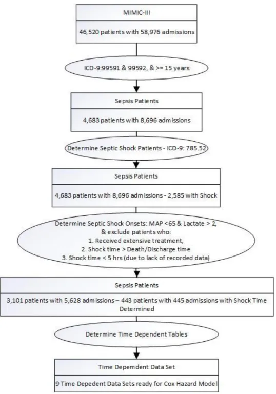
The study used data from the MIMIC-III database v1.3, which is a relational database containing data of ICU patients at Beth Israel Deaconess Medical Center (Goldberger et al., 2000; "MIMIC-III Clinical Database," 2015). MIMIC-III is an open access database developed by the MIT Lab for Computational Physiology, containing de-identified health data for more than 40,000 critical care patients, including demographics, vital signs, laboratory tests, medications, and more (Goldberger et al., 2000; "MIMIC-III Clinical Database," 2015). MIMIC-III is an extension of MIMIC-II and augments it with newly collected data between 2008 – 2012 (Goldberger et al., 2000; "MIMIC-III Clinical Database," 2015). The MIMIC-III database v1.3 has records of 46,520 ICU patients with 58,976 admissions (a patient could have multiple admissions), collected at Beth Israel Deaconess Medical Center between 2001 – 2012 (Goldberger et al., 2000; "MIMIC-III
Clinical Database," 2015). The information included laboratory data, therapeutic intervention profiles such as vasoactive medication drip rates and ventilator settings, nursing progress notes, discharge summaries, radiology reports, provider order entry data, International Classification of Diseases, 9th Revision codes, and, for a subset of patients, high resolution vital sign trends and waveforms (Saeed et al., 2011). The privacy of patients was preserved by removing all Protected Health Information (PHI) in order to comply with Health Insurance Portability and Accountability Act standards (Saeed et al., 2011). The database was opened for free access to researchers on February 2010 through the Internet and was accompanied by a detailed manual and data processing tools (Saeed et al., 2011).
The data of the MIMIC-III is temporal. Most fields are time-stamped. Some fields were updated hourly, while others were updated every four hours. Patients were tracked from the time they entered the ICU, this is time where t=0, until patients got released from the ICU or passed away. The database had 4,683 patients who were diagnosed with sepsis or severe sepsis (ICD-9 codes: 99591 and 99592), and who were 15 years and older. These patients had 8,696 admissions with 2,585 cases resulting in septic shock (ICD-9 code 785.52).
In this dissertation, we treated patients with multiple admissions as separate cases, that is, we included all the admissions of ICUs patients (Verburg, Holman, Dongelmans, de Jonge, & de Keizer, 2018). Each case contributed to the training of the prediction model. The patients’ information and their associated clinical, vital, laboratory test results, and other information were downloaded from the MIT Lab for Computational Physiology as text files, then uploaded to a PostgreSQL database as per instructions and
scripts from the MIT Lab. The required data that included patients’ information, admissions, and chart and lab info were extracted from the PostgreSQL database to a Microsoft SQL Server Database for faster processing. The detailed data selection criteria are shown in figure 1.
2. Features Selection
Based on the literature review and the established medical standards that define septic shock, we started with a comprehensive set of 46 features, which had good
recorded measurements. Only the ones that delivered the best prediction results would be included in the methodology. Table 1 summarizes the list of features:
Table 1
Features that may feed into classifiers
Category Feature Name Feature Description Type Values/Unit Clinical Time since first
antibiotics*
Number of Minutes from time antibiotics was first
administered in the ICU
Numeric Minutes
Clinical 6hr Urine Volume* Total output of urine in the past 6 hours
Numeric mL Clinical Chronic liver disease
and cirrhosis
Presence of chronic liver disease and cirrhosis as specified by ICD-9 code 571
Binary Yes/No
Clinical Cardiac surgery patient
Patient recovering from a cardiac surgery
Binary Yes/No Clinical Immunocompromised A patient who received past
therapy that suppresses resistance to infection as specified by presence of any ICD-9 in V58.65, V58.0, V58.1, 042, 208.0, 202
Binary Yes/No
Clinical SIRS* Currently showing a minimum of two SIRS criteria
Binary Yes/No Clinical Hematological
malignancy
Presence of hematologic malignancy as specified by any ICD-9 code in 200-208
Binary Yes/No
Clinical Chronic heart failure Presence of heart failure as specified by ICD-9 code 428
Binary Yes/No Clinical Chronic organ
insufficiency
Such as chronic liver disease, chronic heart failure, chronic respiratory failure, receiving chronic dialysis as specified by one of the ICD-9 codes 571, 585.6, 428.22, 428.32, 428.42, 518.83
Binary Yes/No
Clinical Diabetes Patience is diabetic as specified by ICD-9 code 250
Clinical Metastatic carcinoma As specified by presence of any ICD-9 codes in 140-165, 170-175, 179-199
Binary Yes/No
Clinical HIV Presence of the human
immunodeficiency virus (HIV)
Binary Yes/No Clinical Dialysis The patient is currently
undergoing dialysis
Binary Yes/No Clinical Chronic renal
insufficiency
The presenceof chronic kidney disease caused by damage to the kidneys
Binary Yes/No
Laboratory BUN/CR* The ratio of BUN/creatinine Numeric 10:1-20:1 Laboratory Arterial pH The pH of the blood measured
by an arterial line
Numeric 7.35-7.45 Laboratory PaO2 Partial pressure of arterial
oxygen
Numeric 75-100 mm Hg Laboratory BUN Blood urea nitrogen Numeric 8-21 mg/dL Laboratory Hepatic SOFA* Hepatic SOFA score
calculated based on the bilirubin concentration
Numeric 1-4
Laboratory WBC White blood cell count Numeric 4-10 x 109/L
Laboratory Renal SOFA* Renal SOFA score calculated on the basis of creatinine concentration
Numeric 1-4
Laboratory Platelets The count of Platelet in the bloodstream
Numeric 150-400 x 109/L
Laboratory Glucose The sugar level in the bloodstream
Numeric 65-110 mg/dL Laboratory Chloride The level of chloride in the
blood
Numeric 95-105 mmol/L Laboratory Lactate The presence of lactic acid in
the body
Numeric 50-150 U/L Laboratory Sodium The level of sodium in the
blood
Numeric 135-145 mmol/L Laboratory PaCO2 The level of Partial pressure of
arterial carbon dioxide
Numeric 35-45 mm Hg Laboratory Creatinine The level of creatinine
(chemical waste product that's produced by your muscle metabolism) in the blood
Numeric 0.8-1.3 mg/dL
Laboratory Potassium The level of potassium in the blood
Numeric 3.5-5 mmol/L Laboratory Hematocrit The percentage of the volume
of whole blood that is made up of red blood cells
Numeric 40%-52% (men), 36%-47% (women) Laboratory Hemoglobin The level of hemoglobin,
which is the protein molecule in red blood cells
Numeric 13-17 g/dL (men), 12-15 g/dL (women) Laboratory Aspartate
aminotransferase
The level of this enzyme in the body
Numeric 5-30 U/L Laboratory C-reactive protein The level of C-reactive protein
(CRP) in the blood
Vital HR Heart rate Numeric 60-100 beats/min Vital SBP Systolic blood pressure Numeric 60-90 mm Hg Vital Shock index* HR/SBP ratio Numeric 0.5-0.7 Vital GCS Glasgow coma score (GCS) Numeric 3-15
Vital RR Respiratory rate Numeric Adults: 12-18 breaths per minute Vital FiO2 Fraction of inspired oxygen Numeric 21%-100%
Vital Neurologic SOFA* Neurologic SOFA score calculated on the basis of GCS
Numeric 1-4 Vital SpO2 The estimation of the oxygen
concentration in the blood
Numeric 96%-100% Vital Admission weight The patient’s weight at
admission
Numeric Kg Vital Hypotension The presence of low blood
pressure symptoms
Binary Yes/No Vital Current weight The continuous measurement
of the patient’s weight Numeric Kg
Vital DBP Diastolic blood pressure Numeric 120-139 mm Hg
Vital Age Age of patient Numeric Years
Note. * Calculated Feature from the electronic health record (EHR)
Additionally, the features listed in Table 2 were extracted from the literature as biomarkers, which can predict septic shock when used individually or as a panel of features. Those features had sparse or no measurements recorded, nevertheless they were listed to raise awareness to start collecting these in future studies.
Table 2
Additional Researched Biomarkers
Biomarker Category IL-1ra Laboratory ICAM-1 Laboratory TNF-α Laboratory Caspase-3 Laboratory IL-8 Laboratory
Procalcitonin (ProCT) Laboratory
Amino-terminal pro-B-type Natriuretic Peptide (NT-proBNP). Laboratory
IL-1β Laboratory
IL-6 Laboratory
IL-10 Laboratory
Lipocalin Laboratory
MMP-9 Laboratory
MMP-10 Laboratory
Tissue Inhibitor of Matrix Metalloproteinases-1 (TIMP-1) Laboratory
TNF-α/IL-10 ratio Calculated
MMP-9/TIMP-1 ratio Calculated
YKL-40 Laboratory
Diastolic Dysfunction (E/é) Clinical
Angiopoietin-1 Laboratory
Angiopoietin-2 Laboratory
sTREM-1, and polymorphonuclear (PMN) CD64 Laboratory
To narrow down the long list, we looked at previous recommendations. Serum lactate was one of the features suggested by many researchers as an indicator of septic shock (Lee & An, 2016; Malmir et al., 2014; Mikkelsen et al., 2009; Phua et al., 2008). Berger et al. (2013) used vital signs such as temperature, heart rate (HR), respiratory rate (RR), mean arterial pressure (MAP), and shock index (SI) as the features to identify septic shock.
Gultepe et al. (2014) utilized temperature, RR, MAP, lactate level, and white blood cells (WBC). As biomarkers for septic shock, Prucha et al. (2015) suggested C-reactive protein, procalcitonin, cytokines, Lipopolysaccharide binding protein (LBP), and WBC. Carrara et al. (2015) proposed 3 different models: first model was based on
temperature, RR, creatinine, lactate, and WBC, the second one used temperature, HR, creatinine, lactate, and WBC, and the third model utilized SBP, DBP, MAP, HR, RR and cardiac output.
GCS, HR, RR, SpO2, temperature, SBP, and DBP were suggested as good
indicators of septic shock (Desautels et al., 2016). Holder et al. (2016) associated low DBP and serum albumin with the progression to septic shock. Sundén-Cullberg et al. (2017) suggested temperature as an indicator of septic shock and concluded that fever slows the process. Modified shock index (MSI) has emerged as an early non-invasive
measure, which is calculated by dividing HR by MAP (Jayaprakash, Gajic, Frank, & Smischney, 2018; Torabi, Moeinaddini, Mirafzal, Rastegari, & Sadeghkhani, 2016). Torabi et al. (2016) introduced a new calculated measure age SI (ageSI), defined as age multiplied by SI, and used it with gender and SBP as predictors. Table 3 summarizes the final set of features.
Table 3
Final Features that were used to feed into classifiers
Category Feature Name Feature Description Type
Laboratory WBC White blood cell count Numeric
Laboratory Lactate The presence of lactic acid in the body Numeric Laboratory Creatinine The level of creatinine (chemical waste product
that's produced by your muscle metabolism) in the blood
Numeric
Laboratory C-reactive protein The level of C-reactive protein (CRP) in the blood
Numeric Laboratory Albumin Albumin test checks liver and kidney function Numeric
Vital HR Heart rate Numeric
Vital SBP Systolic blood pressure Numeric
Vital SI HR/SBP ratio Numeric
Vital GCS Glasgow coma score (GCS) Numeric
Vital RR Respiratory rate Numeric
Vital SpO2 The estimation of the oxygen concentration in
the blood
Numeric
Vital DBP Diastolic blood pressure Numeric
Vital Age Age of patient Numeric
Vital Temperature Body Temperature Numeric
Calculated MAP Mean Arterial Pressure Numeric
Calculated AgeSI SI enhanced with age Numeric
Calculated MSI Modified Shock Index Numeric
3. Data Cleanup and Preparation
MIMIC-III is an extension of MIMIC-II, and inherits all it properties (Goldberger et al., 2000; "MIMIC-III Clinical Database," 2015). The databases have missing values,
duplicate values, and wrongly recorded ones. They required massive attention as they would affect the prediction models (Ho et al., 2012; Ho et al., 2014).
The first step was to extract the data for each feature and place it in a temporary table. The measurements of features were time-stamped, where the time of service was based on the admission date. The difference between the time of measurements and the admission date was binned hourly to unify the measurements across all features
(Desautels et al., 2016; Mao et al., 2018). Outliers and values with wrong data types were eliminated by nulling them out, thus they will be treated as missing values (Ho et al., 2012; Ho et al., 2014). For any hours with multiple values, the mean values were used, and for missing values a carry forward approach was applied, where the latest bin value was propagated till it reached a bin with a value (Desautels et al., 2016; Mao et al., 2018). In case the first value was missing, the imputation followed a carry backward approach (Desautels et al., 2016; Mao et al., 2018).
In the second step, we determined the onset of the septic shock as it was not identified clearly and had to be calculated. As per Singer et al. (2016), the start of septic shock was the first occurrence of: (1) persistent low blood pressure that required the use of vasopressors (compounds that caused the blood vessels to tighten in order to raise blood pressure) to maintain MAP >= 65mmHg, and (2) serum lactate level >2 mmol/L (18mg/dL) even with adequate volume resuscitation. We excluded patients: (1) who received extensive treatment as they would affect the outcome (Henry et al., 2015), (2) whose Shock time > Death/Discharge time, and (3) whose Shock time < 5 hours due to lack of recorded data. The end result was 3,101 patients with 5,628 admissions, which included 443 patients with 445 admissions having septic shock time determined.
The third step was reconstructing the feature tables and transforming them into time-dependent sets (Therneau, Crowson, & Atkinson, 2018). The time-dependent set has the following columns: (a) ID, which defined each subject uniquely; (b) One or more features – one or more columns where each one represented a feature that fed the Cox model; (c) Full Time, which was the time the event or censor (discharge/death) happened; (d) Start – the start of the time bin; (e) Stop – the end of the time bin; and (f) Event, which is the occurrence or not of the event (Therneau et al., 2018). This data frame allowed running the Cox Hazard Model in order to obtain the hazard coefficients for the risk score calculations (Kim, Park, & Kon, 2013). Table 4 illustrated a sample of a time dependent data set for one patient and one feature, where subject_id and hadm_id (hospital admission id) both represented the unique id, Lactate was an input feature, FullTime was the onset of Septic Shock or death/discharge, tStart and tStop were the beginning and end of the hourly time bin, and Shock was the event. The format of a time-dependent data set mandated that at the end of each time bin the event remained zero till the full time was satisfied, then the event would be recorded as either true or false (Therneau et al., 2018).
Table 4
Time Dependent Data Set Sample
subject_id hadm_id Temp RR MAP Lactate WBC FullTime tStart tStop Shock 250 124271 36.39 37 94 1.2 17.6 23 0 1 0 250 124271 36.44 40 94 1.2 17.6 23 1 2 0 250 124271 36.44 38 94 1.2 17.6 23 2 3 0 250 124271 36.67 31 94 1.2 17.6 23 3 4 0 250 124271 37.94 38 94 0.8 17.6 23 4 5 0 250 124271 37.94 39 94 0.8 17.6 23 5 6 0 250 124271 37.94 36 94 0.8 17.6 23 6 7 0 250 124271 37.94 18 94 0.8 17.6 23 7 8 0
250 124271 37.94 23 88 0.8 12.7 23 8 9 0 250 124271 37.94 17 96 0.8 12.7 23 9 10 0 250 124271 37.94 23 77 0.8 12.7 23 10 11 0 250 124271 39 24 90 1.1 12.7 23 11 12 0 250 124271 39 26 97 1.1 12.7 23 12 13 0 250 124271 38.67 24 99 1.1 12.7 23 13 14 0 250 124271 38.67 36 74 1.1 12.7 23 14 15 0 250 124271 36.94 29 101 1.1 12.7 23 15 16 0 250 124271 36.94 33 68 1.1 12.7 23 16 17 0 250 124271 35.67 33 69 1.4 27 23 17 18 0 250 124271 35.67 35 67 1.4 27 23 18 19 0 250 124271 36.44 32 75 1.4 27 23 19 20 0 250 124271 36.44 32 70 3.9 27 23 20 21 0 250 124271 36.5 35 70 3.9 27 23 21 22 0 250 124271 36.5 35 62 3.9 21.5 23 22 23 1
The fourth step was to randomly partition the newly formed dataset into an 80% training set and a 20% test set. For validation purposes, the training set was further partitioned into a 10-fold cross validation sets. Table 5 summarizes the actual numbers of the training and test sets as well as the breakdown of each class.
Table 5
Partitioned Data Sets Detailed Counts (patients with multiple admissions)
Total 0 1
Training Set 4,502 4132 370
Test Set 1126 1051 75
4. Prediction Model
In this dissertation, we developed a prediction model for septic shock based on the features extracted from the MIMIC-III database and were listed in table 3. The prediction model was an extended version of the Random Forest Ensemble called the Cox Enhanced Random Forest (CERF). In this new method, we produced nine preliminary models each consisting of different sets of features from table 3. We generated the Cox hazard
coefficients for each of the nine models. For each model, we calculated Cox risk scores as linear combinations of the features at time t, weighted by multivariate Cox
proportional hazard coefficients (Kim et al., 2013). We added the score to each model and applied the Random Forest ensemble to determine the final classification at t hours before the onset of the shock. We then chose the model that produced the highest accuracy, sensitivity, and specificity as the prediction model for CERF. The detailed steps of the model were as follows:
First step. Based on the literature review, we produced nine preliminary models
consisting of different subsets of features. The features had individually or collectively worked as good predictors of septic shock in previous studies. The preliminary nine models are listed below:
1. Temperature, HR, RR, MAP, and SI (Berger et al., 2013)
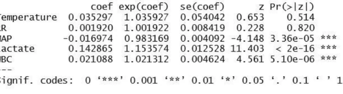
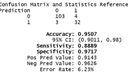
2. Temperature, RR, MAP, Lactate, and WBC (Gultepe et al., 2014)
3. Temperature, RR, Creatinine, Lactate, and WBC (Carrara et al., 2015). 4. Temperature, HR, Creatinine, Lactate, and WBC (Carrara et al., 2015) 5. HR, RR, MAP, SBP, and DBP (Carrara et al., 2015).
6. Temperature, HR, RR, SBP, DBP, SpO2, and GCS (Desautels et al., 2016)
7. DBP and Albumin (Holder et al., 2016) 8. MSI (Jayaprakash et al., 2018)
9. ageSI, Age, SBP, and Gender (Torabi et al., 2016)
Second step. Used the Cox proportional hazards model to obtain the coefficients
(Li, Zhou, Choubey, & Sievenpiper, 2007), based on the nine sets listed in the first step. Each single run was performed on the whole training set for all patients from time of
admission to the time of the event or the censor time (discharged or died without getting the event).
The Cox proportional hazards model is a statistical technique for survival analysis of data (Walters, 2009). Survival models predict hazard at time t as a function of the input variables. In addition, the model allows separating the effects of treatment from other triggering features (Walters, 2009). The Cox proportional hazards (CPH) model is used extensively for survival analysis for censored data (Bonato et al., 2011; Hothorn et al., 2006; Tsujitani et al., 2012). It is one of the most widespread models in statistical analysis (Bonato et al., 2011; Wang et al., 2014). The CPH model is used broadly in clinical studies for risk ratio estimation (Lin et al., 2013). This method had helped researchers achieve good results in medical predictions and risk estimations (Guilloux et al., 2016; Jackson & Cox, 2014; Lee et al., 2016; Tolosie & Sharma, 2014; Wang et al., 2014; Wang et al., 2015; Wu et al., 2016).
The model is specified as follows:
ℎ(𝑡) = ℎ0(𝑡) × 𝑒∑𝑛𝑖=1𝛽𝑖×𝑋𝑖
The quantity h0(t) is the baseline or underlying hazard function and corresponds to the probability of triggering the event, the septic shock, when all the explanatory features are zero (Walters, 2009). Xi represents the ith predictor in the features’ set. The regression coefficients βi give the proportional change in the hazard, related to changes in the
explanatory features. β is assessed with the maximum likelihood estimate (MLE) method, which is the value that makes the feature the most probable. Using the Survival Library in R, the coxph function was used to determine the Cox model including the coefficients (Therneau, 2018).