Regularization Paths for Generalized Linear Models via Coordinate Descent

(1)

January 2010, Volume 33, Issue 1. http://www.jstatsoft.org/

Regularization Paths for Generalized Linear Models

via Coordinate Descent

Jerome Friedman Stanford University Trevor Hastie Stanford University Rob Tibshirani Stanford University Abstract

We develop fast algorithms for estimation of generalized linear models with convex penalties. The models include linear regression, two-class logistic regression, and multi-nomial regression problems while the penalties include`1(the lasso),`2(ridge regression)

and mixtures of the two (the elastic net). The algorithms use cyclical coordinate descent, computed along a regularization path. The methods can handle large problems and can also deal efficiently with sparse features. In comparative timings we find that the new algorithms are considerably faster than competing methods.

Keywords: lasso, elastic net, logistic regression, `1 penalty, regularization path,

coordinate-descent.

1. Introduction

The lasso (Tibshirani 1996) is a popular method for regression that uses an `1 penalty to

achieve a sparse solution. In the signal processing literature, the lasso is also known asbasis pursuit (Chen et al. 1998). This idea has been broadly applied, for example to general-ized linear models (Tibshirani 1996) and Cox’s proportional hazard models for survival data (Tibshirani 1997). In recent years, there has been an enormous amount of research activity devoted to related regularization methods:

1. The grouped lasso (Yuan and Lin 2007;Meieret al.2008), where variables are included or excluded in groups.

2. The Dantzig selector (Candes and Tao 2007, and discussion), a slightly modified version of the lasso.

3. Theelastic net(Zou and Hastie 2005) for correlated variables, which uses a penalty that is part `1, part `2.

(2)

4. `1 regularization paths for generalized linear models (Park and Hastie 2007a).

5. Methods using non-concave penalties, such as SCAD (Fan and Li 2005) and Friedman’s generalized elastic net (Friedman 2008), enforce more severe variable selection than the lasso.

6. Regularization paths for the support-vector machine (Hastie et al. 2004).

7. The graphical lasso (Friedman et al. 2008) for sparse covariance estimation and undi-rected graphs.

Efron et al. (2004) developed an efficient algorithm for computing the entire regularization path for the lasso for linear regression models. Their algorithm exploits the fact that the coef-ficient profiles are piecewise linear, which leads to an algorithm with the same computational cost as the full least-squares fit on the data (see alsoOsborneet al. 2000).

In some of the extensions above (items 2,3, and 6), piecewise-linearity can be exploited as in Efronet al. (2004) to yield efficient algorithms. Rosset and Zhu(2007) characterize the class of problems where piecewise-linearity exists—both the loss function and the penalty have to be quadratic or piecewise linear.

Here we instead focus on cyclical coordinate descent methods. These methods have been proposed for the lasso a number of times, but only recently was their power fully appreciated. Early references includeFu (1998),Shevade and Keerthi (2003) andDaubechieset al.(2004). Van der Kooij(2007) independently used coordinate descent for solving elastic-net penalized regression models. Recent rediscoveries include Friedman et al. (2007) and Wu and Lange (2008). The first paper recognized the value of solving the problem along an entire path of values for the regularization parameters, using the current estimates as warm starts. This strategy turns out to be remarkably efficient for this problem. Several other researchers have also re-discovered coordinate descent, many for solving the same problems we address in this paper—notably Shevade and Keerthi (2003), Krishnapuram and Hartemink (2005), Genkin et al.(2007) and Wuet al. (2009).

In this paper we extend the work of Friedman et al. (2007) and develop fast algorithms for fitting generalized linear models with elastic-net penalties. In particular, our models include regression, two-class logistic regression, and multinomial regression problems. Our algorithms can work on very large datasets, and can take advantage of sparsity in the feature set. We provide a publicly available package glmnet (Friedman et al. 2009) implemented in the R programming system (R Development Core Team 2009). We do not revisit the well-established convergence properties of coordinate descent in convex problems (Tseng 2001) in this article.

Lasso procedures are frequently used in domains with very large datasets, such as genomics and web analysis. Consequently a focus of our research has been algorithmic efficiency and speed. We demonstrate through simulations that our procedures outperform all competitors — even those based on coordinate descent.

In Section2 we present the algorithm for the elastic net, which includes the lasso and ridge regression as special cases. Section3 and 4 discuss (two-class) logistic regression and multi-nomial logistic regression. Comparative timings are presented in Section5.

Although the title of this paper advertises regularization paths for GLMs, we only cover three important members of this family. However, exactly the same technology extends trivially to

(3)

other members of the exponential family, such as the Poisson model. We plan to extend our software to cover these important other cases, as well as the Cox model for survival data. Note that this article is about algorithms for fitting particular families of models, and not about the statistical properties of these models themselves. Such discussions have taken place elsewhere.

2. Algorithms for the lasso, ridge regression and elastic net

We consider the usual setup for linear regression. We have a response variable Y ∈ _R and a predictor vector X ∈ _Rp_{, and we approximate the regression function by a linear model}

E(Y|X =x) = β0 +x>β. We have N observation pairs (xi, yi). For simplicity we assume the xij are standardized:

PN

i=1xij = 0, _N1

PN

i=1x2ij = 1, for j = 1, . . . , p. Our algorithms generalize naturally to the unstandardized case. The elastic net solves the following problem

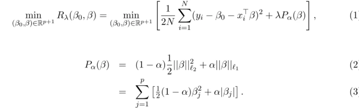
min (β0,β)∈Rp+1 Rλ(β0, β) = min (β0,β)∈Rp+1 " 1 2N N X i=1 (yi−β0−xi>β)2+λPα(β) # , (1) where Pα(β) = (1−α) 1 2||β|| 2 `2+α||β||`1 (2) = p X j=1 ₁ 2(1−α)β 2 j +α|βj| . (3)

Pα is the elastic-net penalty(Zou and Hastie 2005), and is a compromise between the ridge-regression penalty (α = 0) and the lasso penalty (α = 1). This penalty is particularly useful in thepN situation, or any situation where there are many correlated predictor variables.1 Ridge regression is known to shrink the coefficients of correlated predictors towards each other, allowing them to borrow strength from each other. In the extreme case ofk identical predictors, they each get identical coefficients with 1/kth the size that any single one would get if fit alone. From a Bayesian point of view, the ridge penalty is ideal if there are many predictors, and all have non-zero coefficients (drawn from a Gaussian distribution).

Lasso, on the other hand, is somewhat indifferent to very correlated predictors, and will tend to pick one and ignore the rest. In the extreme case above, the lasso problem breaks down. The lasso penalty corresponds to a Laplace prior, which expects many coefficients to be close to zero, and a small subset to be larger and nonzero.

The elastic net withα= 1−εfor some smallε >0 performs much like the lasso, but removes any degeneracies and wild behavior caused by extreme correlations. More generally, the entire family Pα creates a useful compromise between ridge and lasso. As α increases from 0 to 1, for a givenλthe sparsity of the solution to (1) (i.e., the number of coefficients equal to zero) increases monotonically from 0 to the sparsity of the lasso solution.

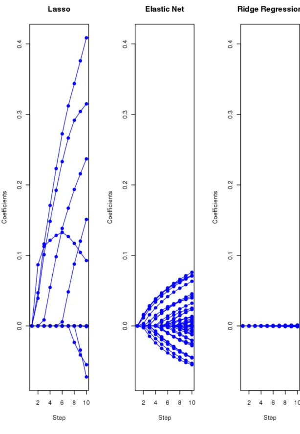
Figure 1 shows an example that demonstrates the effect of varying α. The dataset is from (Golubet al.1999), consisting of 72 observations on 3571 genes measured with DNA microar-rays. The observations fall in two classes, so we use the penalties in conjunction with the

1

Zou and Hastie(2005) called this penalty thenaiveelastic net, and preferred a rescaled version which they

(4)

Figure 1: Leukemiadata: profiles of estimated coefficients for three methods, showing only first 10 steps (values forλ) in each case. For the elastic net,α = 0.2.

(5)

logistic regression models of Section 3. The coefficient profiles from the first 10 steps (grid values forλ) for each of the three regularization methods are shown. The lasso penalty admits at most N = 72 genes into the model, while ridge regression gives all 3571 genes non-zero coefficients. The elastic-net penalty provides a compromise between these two, and has the effect of averaging genes that are highly correlated and then entering the averaged gene into the model. Using the algorithm described below, computation of the entire path of solutions for each method, at 100 values of the regularization parameter evenly spaced on the log-scale, took under a second in total. Because of the large number of non-zero coefficients for the ridge penalty, they are individually much smaller than the coefficients for the other methods. Consider a coordinate descent step for solving (1). That is, suppose we have estimates ˜β0 and

˜

β` for`6=j, and we wish to partially optimize with respect to βj. We would like to compute the gradient at βj = ˜βj, which only exists if ˜βj 6= 0. If ˜βj >0, then

∂Rλ ∂βj |_β_{= ˜}_β =−1 N N X i=1 xij(yi−β˜o−x>i β˜) +λ(1−α)βj+λα. (4)

A similar expression exists if ˜βj <0, and ˜βj = 0 is treated separately. Simple calculus shows (Donoho and Johnstone 1994) that the coordinate-wise update has the form

˜ βj ← S 1 N PN i=1xij(yi−y˜i(j)), λα 1 +λ(1−α) (5) where

y˜_i(j) = ˜β0 +P_`6=jxi`β˜` is the fitted value excluding the contribution from xij, and hence yi −y˜

(j)

i the partial residual for fitting βj. Because of the standardization,

1

N

PN

i=1xij(yi −y˜ (j)

i ) is the simple least-squares coefficient when fitting this partial residual toxij.

S(z, γ) is the soft-thresholding operator with value sign(z)(|z| −γ)+ =    z−γ ifz >0 andγ <|z| z+γ ifz <0 andγ <|z| 0 ifγ ≥ |z|. (6)

The details of this derivation are spelled out in Friedman et al.(2007).

Thus we compute the simple least-squares coefficient on the partial residual, apply soft-thresholding to take care of the lasso contribution to the penalty, and then apply a pro-portional shrinkage for the ridge penalty. This algorithm was suggested by Van der Kooij (2007).

2.1. Naive updates

Looking more closely at (5), we see that

yi−y˜(ij) = yi−yˆi+xijβ˜j

(6)

where ˆyi is the current fit of the model for observationi, and hence ri the current residual. Thus 1 N N X i=1 xij(yi−y˜_i(j)) = 1 N N X i=1 xijri+ ˜βj, (8)

because the xj are standardized. The first term on the right-hand side is the gradient of the loss with respect to βj. It is clear from (8) why coordinate descent is computationally efficient. Many coefficients are zero, remain zero after the thresholding, and so nothing needs to be changed. Such a step costsO(N) operations— the sum to compute the gradient. On the other hand, if a coefficient does change after the thresholding, ri is changed inO(N) and the step costsO(2N). Thus a complete cycle through allpvariables costsO(pN) operations. We refer to this as thenaive algorithm, since it is generally less efficient than thecovariance updating algorithm to follow. Later we use these algorithms in the context of iteratively reweighted least squares (IRLS), where the observation weights change frequently; there the naive algorithm dominates.

2.2. Covariance updates

Further efficiencies can be achieved in computing the updates in (8). We can write the first term on the right (up to a factor 1/N) as

N X i=1 xijri =hxj, yi − X k:|_β˜_k|>0 hxj, xkiβ˜k, (9)

wherehxj, yi=PNi=1xijyi. Hence we need to compute inner products of each feature withy initially, and then each time a new feature xk enters the model (for the first time), we need to compute and store its inner product with all the rest of the features (O(N p) operations). We also store thepgradient components (9). If one of the coefficients currently in the model changes, we can update each gradient inO(p) operations. Hence with m non-zero terms in the model, a complete cycle costsO(pm) operations if no new variables become non-zero, and costsO(N p) for each new variable entered. Importantly, O(N) calculations do not have to be made at every step. This is the case for all penalized procedures with squared error loss. 2.3. Sparse updates

We are sometimes faced with problems where theN×pfeature matrixXis extremely sparse. A leading example is from document classification, where the feature vector uses the so-called “bag-of-words” model. Each document is scored for the presence/absence of each of the words in the entire dictionary under consideration (sometimes counts are used, or some transformation of counts). Since most words are absent, the feature vector for each document is mostly zero, and so the entire matrix is mostly zero. We store such matrices efficiently in

sparse column format, where we store only the non-zero entries and the coordinates where they occur.

Coordinate descent is ideally set up to exploit such sparsity, in an obvious way. TheO(N) inner-product operations in either the naive or covariance updates can exploit the sparsity, by summing over only the non-zero entries. Note that in this case scaling of the variables will

(7)

not alter the sparsity, but centering will. So scaling is performed up front, but the centering is incorporated in the algorithm in an efficient and obvious manner.

2.4. Weighted updates

Often a weight wi (other than 1/N) is associated with each observation. This will arise naturally in later sections where observations receive weights in the IRLS algorithm. In this case the update step (5) becomes only slightly more complicated:

˜ βj ← SPN i=1wixij(yi−y˜i(j)), λα PN i=1wix2ij +λ(1−α) . (10)

If the xj are not standardized, there is a similar sum-of-squares term in the denominator (even without weights). The presence of weights does not change the computational costs of either algorithm much, as long as the weights remain fixed.

2.5. Pathwise coordinate descent

We compute the solutions for a decreasing sequence of values for λ, starting at the smallest value λmax for which the entire vector ˆβ = 0. Apart from giving us a path of solutions, this

scheme exploitswarm starts, and leads to a more stable algorithm. We have examples where it is faster to compute the path down to λ(for smallλ) than the solution only at that value for λ.

When ˜β = 0, we see from (5) that ˜βj will stay zero if _N1|hxj, yi| < λα. Hence N αλmax =

max`|hx`, yi|. Our strategy is to select a minimum value λmin = λmax, and construct a

sequence ofK values of λ decreasing fromλmax toλmin on the log scale. Typical values are

= 0.001 andK = 100.

2.6. Other details

Irrespective of whether the variables are standardized to have variance 1, we always center each predictor variable. Since the intercept is not regularized, this means that ˆβ0 = ¯y, the

mean of the yi, for all values ofα and λ.

It is easy to allow different penalties λj for each of the variables. We implement this via a penalty scaling parameter γj ≥ 0. If γj > 0, then the penalty applied to βj is λj = λγj. If γj = 0, that variable does not get penalized, and always enters the model unrestricted at the first step and remains in the model. Penalty rescaling would also allow, for example, our software to be used to implement the adaptive lasso(Zou 2006).

Considerable speedup is obtained by organizing the iterations around theactive setof features— those with nonzero coefficients. After a complete cycle through all the variables, we iterate on only the active set till convergence. If another complete cycle does not change the active set, we are done, otherwise the process is repeated. Active-set convergence is also mentioned in Meieret al. (2008) and Krishnapuram and Hartemink (2005).

(8)

3. Regularized logistic regression

When the response variable is binary, the linear logistic regression model is often used. Denote by G the response variable, taking values in G = {1,2} (the labeling of the elements is arbitrary). The logistic regression model represents the class-conditional probabilities through a linear function of the predictors

Pr(G= 1|x) = 1

1 +e−(β0+x>β), (11) Pr(G= 2|x) = 1

1 +e+(β0+x>β) = 1−Pr(G= 1|x).

Alternatively, this implies that

logPr(G= 1|x)

Pr(G= 2|x) =β0+x

>_β. ₍₁₂₎

Here we fit this model by regularized maximum (binomial) likelihood. Let p(xi) = Pr(G= 1|xi) be the probability (11) for observationiat a particular value for the parameters (β0, β),

then we maximize the penalized log likelihood max (β0,β)∈Rp+1 " 1 N N X i=1 I(gi = 1) logp(xi) +I(gi= 2) log(1−p(xi)) −λPα(β) # . (13)

Denoting yi =I(gi = 1), the log-likelihood part of (13) can be written in the more explicit form `(β0, β) = 1 N N X i=1 yi·(β0+x>i β)−log(1 +e(β0+x > iβ)), (14)

a concave function of the parameters. The Newton algorithm for maximizing the (unpe-nalized) log-likelihood (14) amounts to iteratively reweighted least squares. Hence if the current estimates of the parameters are ( ˜β0,β˜), we form a quadratic approximation to the

log-likelihood (Taylor expansion about current estimates), which is

`Q(β0, β) =− 1 2N N X i=1 wi(zi−β0−x>i β)2+C( ˜β0,β˜)2 (15) where zi = β˜0+x>i β˜+ yi−p˜(xi) ˜ p(xi)(1−p˜(xi)) , (working response) (16) wi = p˜(xi)(1−p˜(xi)), (weights) (17)

and ˜p(xi) is evaluated at the current parameters. The last term is constant. The Newton update is obtained by minimizing`Q.

Our approach is similar. For each value of λ, we create an outer loop which computes the quadratic approximation `Q about the current parameters ( ˜β0,β˜). Then we use coordinate

descent to solve the penalized weighted least-squares problem min

(β0,β)∈Rp+1

{−`Q(β0, β) +λPα(β)}. (18) This amounts to a sequence of nested loops:

(9)

outer loop: Decrementλ.

middle loop: Update the quadratic approximation `Q using the current parameters ( ˜β0,β˜). inner loop: Run the coordinate descent algorithm on the penalized weighted-least-squares

problem (18).

There are several important details in the implementation of this algorithm.

When p N, one cannot run λ all the way to zero, because the saturated logistic regression fit is undefined (parameters wander off to±∞in order to achieve probabilities of 0 or 1). Hence the default λsequence runs down toλmin=λmax>0.

Care is taken to avoid coefficients diverging in order to achieve fitted probabilities of 0 or 1. When a probability is within ε= 10−5 of 1, we set it to 1, and set the weights to

ε. 0 is treated similarly.

Our code has an option to approximate the Hessian terms by an exact upper-bound. This is obtained by setting thewiin (17) all equal to 0.25 (Krishnapuram and Hartemink 2005).

We allow the response data to be supplied in the form of a two-column matrix of counts, sometimes referred to as grouped data. We discuss this in more detail in Section4.2. The Newton algorithm is not guaranteed to converge without step-size optimization

(Leeet al. 2006). Our code does not implement any checks for divergence; this would slow it down, and when used as recommended we do not feel it is necessary. We have a closed form expression for the starting solutions, and each subsequent solution is warm-started from the previous close-by solution, which generally makes the quadratic approximations very accurate. We have not encountered any divergence problems so far.

4. Regularized multinomial regression

When the categorical response variable G has K > 2 levels, the linear logistic regression model can be generalized to a multi-logit model. The traditional approach is to extend (12) toK−1 logits

log Pr(G=`|x)

Pr(G=K|x) =β0`+x

>_β

`, `= 1, . . . , K −1. (19)

Here β` is a p-vector of coefficients. As in Zhu and Hastie (2004), here we choose a more symmetric approach. We model

Pr(G=`|x) = e β0`+x>β` PK k=1eβ0k+x >_β k (20) This parametrization is not estimable without constraints, because for any values for the parameters {β0`, β`}K1 , {β0`−c0, β` −c}K1 give identical probabilities (20). Regularization

(10)

We fit the model (20) by regularized maximum (multinomial) likelihood. Using a similar notation as before, let p`(xi) = Pr(G=`|xi), and let gi ∈ {1,2, . . . , K} be the ith response. We maximize the penalized log-likelihood

max {β0`,β`}K1∈RK(p+1) " 1 N N X i=1 logpgi(xi)−λ K X `=1 Pα(β`) # . (21)

Denote byY the N ×K indicator response matrix, with elements yi`=I(gi =`). Then we can write the log-likelihood part of (21) in the more explicit form

`({β0`, β`}K1 ) = 1 N N X i=1 " _K X `=1 yi`(β0`+x>i β`)−log K X `=1 eβ0`+x>iβ` !# . (22)

The Newton algorithm for multinomial regression can be tedious, because of the vector nature of the response observations. Instead of weights wi as in (17), we get weight matrices, for example. However, in the spirit of coordinate descent, we can avoid these complexities. We perform partial Newton steps by forming a partial quadratic approximation to the log-likelihood (22), allowing only (β0`, β`) to vary for a single class at a time. It is not hard to show that this is

`Q`(β0`, β`) =− 1 2N N X i=1 wi`(zi`−β0`−x>i β`)2+C({β˜0k,β˜k}K1 ), (23) where as before zi` = β˜0`+x>i β˜`+ yi`−p˜`(xi) ˜ p`(xi)(1−p˜`(xi)) , (24) wi` = p˜`(xi)(1−p˜`(xi)), (25)

Our approach is similar to the two-class case, except now we have to cycle over the classes as well in the outer loop. For each value ofλ, we create an outer loop which cycles over `

and computes the partial quadratic approximation `Q` about the current parameters ( ˜β0,β˜).

Then we use coordinate descent to solve the penalized weighted least-squares problem min

(β0`,β`)∈Rp+1

{−`Q`(β0`, β`) +λPα(β`)}. (26)

This amounts to the sequence of nested loops: outer loop: Decrementλ.

middle loop (outer): Cycle over`∈ {1,2, . . . , K,1,2. . .}.

middle loop (inner): Update the quadratic approximation `Q` using the current parame-ters {β˜0k,β˜k}K1 .

inner loop: Run the co-ordinate descent algorithm on the penalized weighted-least-squares problem (26).

(11)

4.1. Regularization and parameter ambiguity

As was pointed out earlier, if {β0`, β`}1K characterizes a fitted model for (20), then {β0`−

c0, β`−c}K1 gives an identical fit (cis ap-vector). Although this means that the log-likelihood

part of (21) is insensitive to (c0, c), the penalty is not. In particular, we can always improve

an estimate{β0`, β`}K1 (w.r.t. (21)) by solving min c∈Rp K X `=1 Pα(β`−c). (27)

This can be done separately for each coordinate, hence

cj = arg min t K X `=1 ₁ 2(1−α)(βj`−t) 2₊_α_|_β j`−t| . (28)

Theorem 1 Consider problem (28) for values α∈[0,1]. Let β¯j be the mean of theβj`, and

β_jM a median of theβj` (and for simplicity assume β¯j ≤β_jM. Then we have

cj ∈[ ¯βj, βjM], (29)

with the left endpoint achieved if α= 0, and the right if α= 1.

The two endpoints are obvious. The proof of Theorem 1 is given in Appendix A. A con-sequence of the theorem is that a very simple search algorithm can be used to solve (28). The objective is piecewise quadratic, with knots defined by the βj`. We need only evaluate solutions in the intervals including the mean and median, and those in between. We recenter

the parameters in each index set j after eachinner middle loop step, using the the solution

cj for eachj.

Not all the parameters in our model are regularized. The interceptsβ0` are not, and with our penalty modifiers γj (Section 2.6) others need not be as well. For these parameters we use mean centering.

4.2. Grouped and matrix responses

As in the two class case, the data can be presented in the form of a N ×K matrix mi` of non-negative numbers. For example, if the data are grouped: at each xi we have a number of multinomial samples, with mi` falling into category `. In this case we divide each row by the row-sum mi =P`mi`, and produce our response matrix yi` =mi`/mi. mi becomes an observation weight. Our penalized maximum likelihood algorithm changes in a trivial way. The working response (24) is defined exactly the same way (using yi` just defined). The weights in (25) get augmented with the observation weightmi:

wi`=mip˜`(xi)(1−p˜`(xi)). (30)

Equivalently, the data can be presented directly as a matrix of class proportions, along with a weight vector. From the point of view of the algorithm, any matrix of positive numbers and any non-negative weight vector will be treated in the same way.

(12)

5. Timings

In this section we compare the run times of the coordinate-wise algorithm to some competing algorithms. These use the lasso penalty (α= 1) in both the regression and logistic regression settings. All timings were carried out on an Intel Xeon 2.80GH processor.

We do not perform comparisons on the elastic net versions of the penalties, since there is not much software available for elastic net. Comparisons of ourglmnet code with theR package elasticnet will mimic the comparisons with lars (Hastie and Efron 2007) for the lasso, since elasticnet (Zou and Hastie 2004) is built on thelarspackage.

5.1. Regression with the lasso

We generated Gaussian data withN observations andppredictors, with each pair of predictors

Xj, Xj0 having the same population correlation ρ. We tried a number of combinations of N

and p, withρ varying from zero to 0.95. The outcome values were generated by

Y =

p

X

j=1

Xjβj+k·Z (31)

whereβj = (−1)jexp(−2(j−1)/20),Z ∼N(0,1) and k is chosen so that the signal-to-noise ratio is 3.0. The coefficients are constructed to have alternating signs and to be exponentially decreasing.

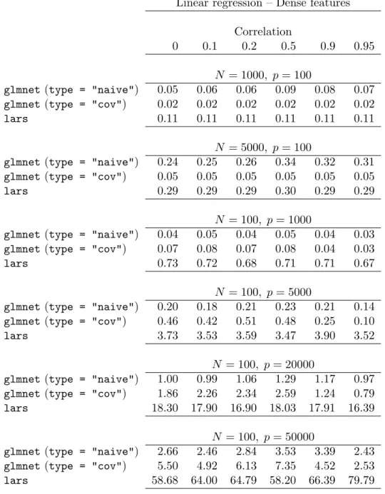
Table1shows the average CPU timings for the coordinate-wise algorithm, and thelars proce-dure (Efronet al.2004). All algorithms are implemented asRfunctions. The coordinate-wise algorithm does all of its numerical work inFortran, while lars (Hastie and Efron 2007) does much of its work in R, calling Fortran routines for some matrix operations. However com-parisons inFriedmanet al. (2007) showed thatlars was actually faster than a version coded entirely inFortran. Comparisons between different programs are always tricky: in particular thelarsprocedure computes the entire path of solutions, while the coordinate-wise procedure solves the problem for a set of pre-defined points along the solution path. In the orthogonal case, lars takes min(N, p) steps: hence to make things roughly comparable, we called the latter two algorithms to solve a total of min(N, p) problems along the path. Table 1 shows timings in seconds averaged over three runs. We see that glmnet is considerably faster than lars; the covariance-updating version of the algorithm is a little faster than the naive version

whenN > pand a little slower whenp > N. We had expected that high correlation between

the features would increase the run time ofglmnet, but this does not seem to be the case. 5.2. Lasso-logistic regression

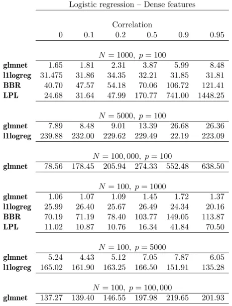
We used the same simulation setup as above, except that we took the continuous outcomey, defined p = 1/(1 + exp(−y)) and used this to generate a two-class outcome z with Pr(z = 1) =p, Pr(z = 0) = 1−p. We compared the speed of glmnet to the interior point method l1logreg (Koh et al. 2007b,a), Bayesian binary regression (BBR, Madigan and Lewis 2007; Genkinet al.2007), and the lasso penalized logistic programLPLsupplied by Ken Lange (see Wu and Lange 2008). The latter two methods also use a coordinate descent approach. The BBR software automatically performs ten-fold cross-validation when given a set of λ

(13)

Linear regression – Dense features Correlation

0 0.1 0.2 0.5 0.9 0.95

N = 1000, p= 100

glmnet (type = "naive") 0.05 0.06 0.06 0.09 0.08 0.07 glmnet (type = "cov") 0.02 0.02 0.02 0.02 0.02 0.02

lars 0.11 0.11 0.11 0.11 0.11 0.11

N = 5000, p= 100

lars 0.29 0.29 0.29 0.30 0.29 0.29

N = 100, p= 1000

lars 0.73 0.72 0.68 0.71 0.71 0.67

N = 100, p= 5000

lars 3.73 3.53 3.59 3.47 3.90 3.52

N = 100, p= 20000

lars 18.30 17.90 16.90 18.03 17.91 16.39

N = 100, p= 50000

lars 58.68 64.00 64.79 58.20 66.39 79.79

Table 1: Timings (in seconds) forglmnet andlars algorithms for linear regression with lasso penalty. The first line is glmnet using naive updating while the second uses covariance updating. Total time for 100λvalues, averaged over 3 runs.

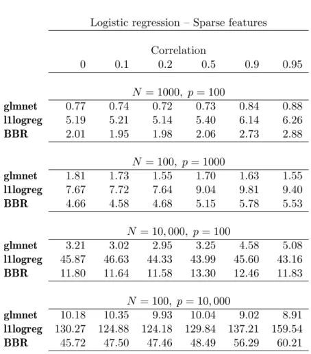
same 100 λ values for all. Table 2 shows the results; in some cases, we omitted a method when it was seen to be very slow at smaller values for N orp. Again we see that glmnet is the clear winner: it slows down a little under high correlation. The computation seems to be roughly linear inN, but grows faster than linear in p. Table 3 shows some results when the feature matrix is sparse: we randomly set 95% of the feature values to zero. Again, the glmnetprocedure is significantly faster than l1logreg.

(14)

Logistic regression – Dense features Correlation 0 0.1 0.2 0.5 0.9 0.95 N = 1000, p= 100 glmnet 1.65 1.81 2.31 3.87 5.99 8.48 l1logreg 31.475 31.86 34.35 32.21 31.85 31.81 BBR 40.70 47.57 54.18 70.06 106.72 121.41 LPL 24.68 31.64 47.99 170.77 741.00 1448.25 N = 5000, p= 100 glmnet 7.89 8.48 9.01 13.39 26.68 26.36 l1logreg 239.88 232.00 229.62 229.49 22.19 223.09 N = 100,000, p= 100 glmnet 78.56 178.45 205.94 274.33 552.48 638.50 N = 100, p= 1000 glmnet 1.06 1.07 1.09 1.45 1.72 1.37 l1logreg 25.99 26.40 25.67 26.49 24.34 20.16 BBR 70.19 71.19 78.40 103.77 149.05 113.87 LPL 11.02 10.87 10.76 16.34 41.84 70.50 N = 100, p= 5000 glmnet 5.24 4.43 5.12 7.05 7.87 6.05 l1logreg 165.02 161.90 163.25 166.50 151.91 135.28 N = 100, p= 100,000 glmnet 137.27 139.40 146.55 197.98 219.65 201.93

Table 2: Timings (seconds) for logistic models with lasso penalty. Total time for tenfold cross-validation over a grid of 100λvalues.

5.3. Real data

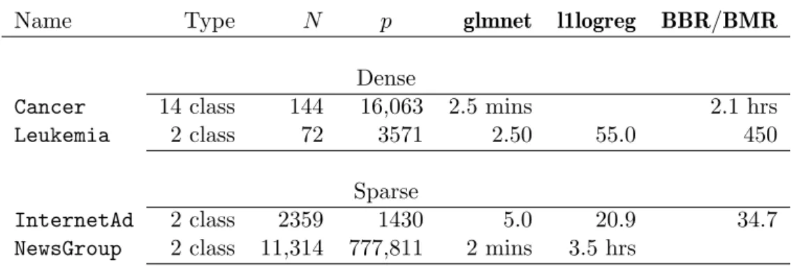
Table4 shows some timing results for four different datasets.

Cancer (Ramaswamyet al.2002): gene-expression data with 14 cancer classes. Here we compare glmnet withBMR(Genkin et al. 2007), a multinomial version ofBBR. Leukemia (Golub et al. 1999): gene-expression data with a binary response indicating

type of leukemia—AMLvs ALL. We used the preprocessed data ofDettling(2004). InternetAd (Kushmerick 1999): document classification problem with mostly binary

features. The response is binary, and indicates whether the document is an advertise-ment. Only 1.2% nonzero values in the predictor matrix.

(15)

Logistic regression – Sparse features Correlation 0 0.1 0.2 0.5 0.9 0.95 N = 1000, p= 100 glmnet 0.77 0.74 0.72 0.73 0.84 0.88 l1logreg 5.19 5.21 5.14 5.40 6.14 6.26 BBR 2.01 1.95 1.98 2.06 2.73 2.88 N = 100, p= 1000 glmnet 1.81 1.73 1.55 1.70 1.63 1.55 l1logreg 7.67 7.72 7.64 9.04 9.81 9.40 BBR 4.66 4.58 4.68 5.15 5.78 5.53 N = 10,000, p= 100 glmnet 3.21 3.02 2.95 3.25 4.58 5.08 l1logreg 45.87 46.63 44.33 43.99 45.60 43.16 BBR 11.80 11.64 11.58 13.30 12.46 11.83 N = 100, p= 10,000 glmnet 10.18 10.35 9.93 10.04 9.02 8.91 l1logreg 130.27 124.88 124.18 129.84 137.21 159.54 BBR 45.72 47.50 47.46 48.49 56.29 60.21

Table 3: Timings (seconds) for logistic model with lasso penalty and sparse features (95% zero). Total time for ten-fold cross-validation over a grid of 100λvalues.

NewsGroup (Lang 1995): document classification problem. We used the training set cultured from these data by Koh et al.(2007a). The response is binary, and indicates a subclass of topics; the predictors are binary, and indicate the presence of particular tri-gram sequences. The predictor matrix has 0.05% nonzero values.

All four datasets are available online with this publication as savedRdata objects (the latter two in sparse format using theMatrixpackage, Bates and Maechler 2009).

For theLeukemiaand InternetAddatasets, theBBRprogram used fewer than 100λvalues so we estimated the total time by scaling up the time for smaller number of values. The InternetAd and NewsGroup datasets are both sparse: 1% nonzero values for the former, 0.05% for the latter. Againglmnet is considerably faster than the competing methods. 5.4. Other comparisons

When making comparisons, one invariably leaves out someones favorite method. We left out our own glmpath (Park and Hastie 2007b) extension of lars for GLMs (Park and Hastie 2007a), since it does not scale well to the size problems we consider here. Two referees of

(16)

Name Type N p glmnet l1logreg BBR/BMR Dense

Cancer 14 class 144 16,063 2.5 mins 2.1 hrs

Leukemia 2 class 72 3571 2.50 55.0 450

Sparse

InternetAd 2 class 2359 1430 5.0 20.9 34.7

NewsGroup 2 class 11,314 777,811 2 mins 3.5 hrs

Table 4: Timings (seconds, unless stated otherwise) for some real datasets. For theCancer, Leukemiaand InternetAd datasets, times are for ten-fold cross-validation using 100 values ofλ; forNewsGroupwe performed a single run with 100 values of λ, withλmin= 0.05λmax.

MacBook Pro HP Linux server

glmnet 0.34 0.13

penalized 10.31

OWL-QN 314.35

Table 5: Timings (seconds) for the Leukemia dataset, using 100 λ values. These timings were performed on two different platforms, which were different again from those used in the earlier timings in this paper.

an earlier draft of this paper suggested two methods of which we were not aware. We ran a single benchmark against each of these using theLeukemiadata, fitting models at 100 values ofλin each case.

OWL-QN: Orthant-Wise Limited-memory Quasi-Newton Optimizer for `1-regularized

Objectives (Andrew and Gao 2007a,b). The software is written in C++, and available from the authors upon request.

The Rpackage penalized(Goeman 2009b,a), which fits GLMs using a fast implementa-tion of gradient ascent.

Table5 shows these comparisons (on two different machines); glmnet is considerably faster in both cases.

6. Selecting the tuning parameters

The algorithms discussed in this paper compute an entire path of solutions (in λ) for any particular model, leaving the user to select a particular solution from the ensemble. One general approach is to use prediction error to guide this choice. If a user is data rich, they can set aside some fraction (say a third) of their data for this purpose. They would then evaluate the prediction performance at each value ofλ, and pick the model with the best performance.

(17)

−6 −5 −4 −3 −2 −1 0 24 26 28 30 32 log(Lambda)

Mean Squared Error

● ● ● ● ● ● ● ● ● ● ● ● ● ● ● ● ● ● ● ● ● ● ● ● ● ● ● ● ● ● ● ● ● ● ● ● ● ● ● ● ● ● ● ● ● ● ● ● ● ● ● ● ● ● ● ● ● ● ● ● ● ● ● ● ● ● ● ● ● ● ● ● ● ● 99 99 97 95 93 75 54 21 12 5 2 1 Gaussian Family −9 −8 −7 −6 −5 −4 −3 −2 0.8 0.9 1.0 1.1 1.2 1.3 1.4 log(Lambda) De viance ● ● ● ● ● ● ● ● ● ● ● ● ● ● ● ● ● ● ● ● ● ● ● ● ● ● ● ● ● ● ● ● ● ● ● ● ● ● ● ● ● ● ● ● ● ● ● ● ● ● ● ● ● ● ● ● ● ● ● ● ● ● ● ● ● ● ● ● ● ● ● ● ● ● ● ● ● 100 98 97 88 74 55 30 9 7 3 2 Binomial Family −9 −8 −7 −6 −5 −4 −3 −2 0.20 0.30 0.40 0.50 log(Lambda) Misclassification Error ● ● ● ● ● ● ● ● ● ● ● ● ● ● ● ● ● ● ● ● ● ● ● ● ● ● ● ● ● ● ● ● ● ● ● ● ● ● ● ● ● ● ● ● ● ● ● ● ● ● ● ● ● ● ● ● ● ● ● ● ● ● ● ● ● ● ● ● ● ● ● ● ● ● ● ● ● 100 98 97 88 74 55 30 9 7 3 2 Binomial Family

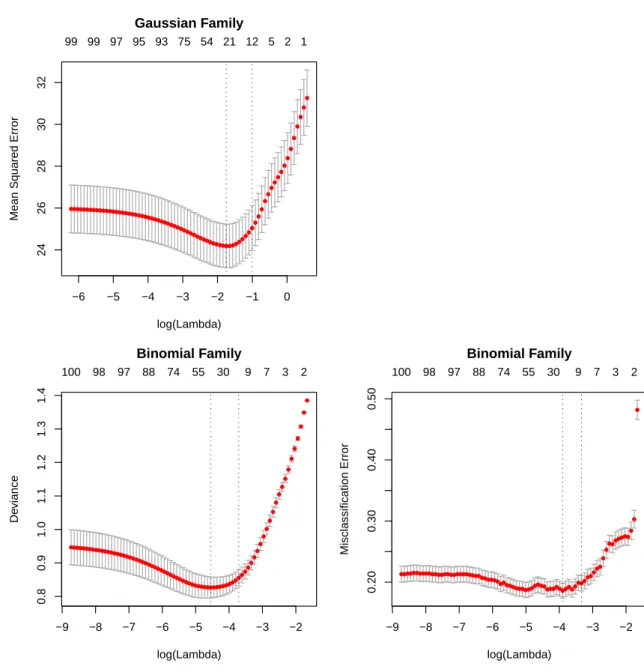
Figure 2: Ten-fold cross-validation on simulated data. The first row is for regression with a Gaussian response, the second row logistic regression with a binomial response. In both cases we have 1000 observations and 100 predictors, but the response depends on only 10 predictors. For regression we use mean-squared prediction error as the measure of risk. For logistic regression, the left panel shows the mean deviance (minus twice the log-likelihood on the left-out data), while the right panel shows misclassification error, which is a rougher measure. In all cases we show the mean cross-validated error curve, as well as a one-standard-deviation band. In each figure the left vertical line corresponds to the minimum error, while the right vertical line the largest value of lambda such that the error is within one standard-error of the minimum—the so called “one-standard-error” rule. The top of each plot is annotated with the size of the models.

(18)

Alternatively, they can use K-fold cross-validation (Hastie et al. 2009, for example), where the training data is used both for training and testing in an unbiased way.

Figure2 illustrates cross-validation on a simulated dataset. For logistic regression, we some-times use the binomial deviance rather than misclassification error, since the latter is smoother. We often use the “one-standard-error” rule when selecting the best model; this acknowledges the fact that the risk curves are estimated with error, so errs on the side of parsimony (Hastie et al.2009). Cross-validation can be used to selectα as well, although it is often viewed as a higher-level parameter and chosen on more subjective grounds.

7. Discussion

Cyclical coordinate descent methods are a natural approach for solving convex problems with`1 or`2 constraints, or mixtures of the two (elastic net). Each coordinate-descent step

is fast, with an explicit formula for each coordinate-wise minimization. The method also exploits the sparsity of the model, spending much of its time evaluating only inner products for variables with non-zero coefficients. Its computational speed both for large N and p are quite remarkable.

An R-language package glmnet is available under general public licence (GPL-2) from the ComprehensiveRArchive Network athttp://CRAN.R-project.org/package=glmnet. Sparse data inputs are handled by theMatrixpackage. MATLABfunctions (Jiang 2009) are available fromhttp://www-stat.stanford.edu/~tibs/glmnet-matlab/.

Acknowledgments

We would like to thank Holger Hoefling for helpful discussions, and Hui Jiang for writing the

MATLABinterface to our Fortranroutines. We thank the associate editor, production editor

and two referees who gave useful comments on an earlier draft of this article.

Friedman was partially supported by grant DMS-97-64431 from the National Science Foun-dation. Hastie was partially supported by grant DMS-0505676 from the National Science Foundation, and grant 2R01 CA 72028-07 from the National Institutes of Health. Tibshirani was partially supported by National Science Foundation Grant DMS-9971405 and National Institutes of Health Contract N01-HV-28183.

References

Andrew G, Gao J (2007a). OWL-QN: Orthant-Wise Limited-Memory Quasi-Newton Op-timizer for L1-Regularized Objectives. URL http://research.microsoft.com/en-us/ downloads/b1eb1016-1738-4bd5-83a9-370c9d498a03.

Andrew G, Gao J (2007b). “Scalable Training of L1-Regularized Log-Linear Models.” In

ICML ’07: Proceedings of the 24th International Conference on Machine Learning, pp. 33–40. ACM, New York, NY, USA. doi:10.1145/1273496.1273501.

Bates D, Maechler M (2009). Matrix: Sparse and Dense Matrix Classes and Methods.

(19)

Candes E, Tao T (2007). “The Dantzig Selector: Statistical Estimation When p is much Larger thann.”The Annals of Statistics,35(6), 2313–2351.

Chen SS, Donoho D, Saunders M (1998). “Atomic Decomposition by Basis Pursuit.” SIAM Journal on Scientific Computing,20(1), 33–61.

Daubechies I, Defrise M, De Mol C (2004). “An Iterative Thresholding Algorithm for Lin-ear Inverse Problems with a Sparsity Constraint.” Communications on Pure and Applied Mathematics,57, 1413–1457.

Dettling M (2004). “BagBoosting for Tumor Classification with Gene Expression Data.”

Bioinformatics,20, 3583–3593.

Donoho DL, Johnstone IM (1994). “Ideal Spatial Adaptation by Wavelet Shrinkage.”

Biometrika,81, 425–455.

Efron B, Hastie T, Johnstone I, Tibshirani R (2004). “Least Angle Regression.”The Annals of Statistics,32(2), 407–499.

Fan J, Li R (2005). “Variable Selection via Nonconcave Penalized Likelihood and its Oracle Properties.”Journal of the American Statistical Association,96, 1348–1360.

Friedman J (2008). “Fast Sparse Regression and Classification.” Technical report, Depart-ment of Statistics, Stanford University. URLhttp://www-stat.stanford.edu/~jhf/ftp/ GPSpub.pdf.

Friedman J, Hastie T, Hoefling H, Tibshirani R (2007). “Pathwise Coordinate Optimization.”

The Annals of Applied Statistics,2(1), 302–332.

Friedman J, Hastie T, Tibshirani R (2008). “Sparse Inverse Covariance Estimation with the Graphical Lasso.”Biostatistics,9, 432–441.

Friedman J, Hastie T, Tibshirani R (2009). glmnet: Lasso and Elastic-Net Regularized Generalized Linear Models. Rpackage version 1.1-4, URLhttp://CRAN.R-project.org/ package=glmnet.

Fu W (1998). “Penalized Regressions: The Bridge vs. the Lasso.”Journal of Computational and Graphical Statistics,7(3), 397–416.

Genkin A, Lewis D, Madigan D (2007). “Large-scale Bayesian Logistic Regression for Text Categorization.”Technometrics,49(3), 291–304.

Goeman J (2009a). “L1 Penalized Estimation in the Cox Proportional Hazards Model.”

Biometrical Journal. doi:10.1002/bimj.200900028. Forthcoming.

Goeman J (2009b). penalized: L1 (Lasso) and L2 (Ridge) Penalized Estimation in GLMs and in the Cox Model. R package version 0.9-27, URL http://CRAN.R-project.org/ package=penalized.

Golub T, Slonim DK, Tamayo P, Huard C, Gaasenbeek M, Mesirov JP, Coller H, Loh ML, Downing JR, Caligiuri MA, Bloomfield CD, Lander ES (1999). “Molecular Classification of Cancer: Class Discovery and Class Prediction by Gene Expression Monitoring.” Science, 286, 531–536.

(20)

Hastie T, Efron B (2007). lars: Least Angle Regression, Lasso and Forward Stagewise.

Rpackage version 0.9-7, URL http://CRAN.R-project.org/package=Matrix.

Hastie T, Rosset S, Tibshirani R, Zhu J (2004). “The Entire Regularization Path for the Support Vector Machine.”Journal of Machine Learning Research,5, 1391–1415.

Hastie T, Tibshirani R, Friedman J (2009). The Elements of Statistical Learning: Prediction, Inference and Data Mining. 2nd edition. Springer-Verlag, New York.

Jiang H (2009). “A MATLABImplementation ofglmnet.” Stanford University, URL http:: //www-stat.stanford.edu/~tibs/glmnet-matlab/.

Koh K, Kim SJ, Boyd S (2007a). “An Interior-Point Method for Large-Scale L1-Regularized Logistic Regression.”Journal of Machine Learning Research,8, 1519–1555.

Koh K, Kim SJ, Boyd S (2007b). l1logreg: A Solver for L1-Regularized Logistic Regression.

Rpackage version 0.1-1. Avaliable from Kwangmoo Koh ([email protected]).

Krishnapuram B, Hartemink AJ (2005). “Sparse Multinomial Logistic Regression: Fast Al-gorithms and Generalization Bounds.” IEEE Transactions on Pattern Analysis and Ma-chine Intelligence, 27(6), 957–968. Fellow-Lawrence Carin and Senior Member-Mario A. T. Figueiredo.

Kushmerick N (1999). “Learning to Remove Internet Advertisements.” In AGENTS ’99: Proceedings of the Third Annual Conference on Autonomous Agents, pp. 175–181. ACM, New York, NY, USA. ISBN 1-58113-066-X. doi:10.1145/301136.301186.

Lang K (1995). “NewsWeeder: Learning to Filter Netnews.” In A Prieditis, S Russell (eds.),

Proceedings of the 12th International Conference on Machine Learning, pp. 331–339. San Francisco.

Lee S, Lee H, Abbeel P, Ng A (2006). “Efficient L1 Logistic Regression.” In Proceedings of the Twenty-First National Conference on Artificial Intelligence (AAAI-06). URL https: //www.aaai.org/Papers/AAAI/2006/AAAI06-064.pdf.

Madigan D, Lewis D (2007).BBR,BMR: Bayesian Logistic Regression. Open-source stand-alone software, URLhttp://www.bayesianregression.org/.

Meier L, van de Geer S, B¨uhlmann P (2008). “The Group Lasso for Logistic Regression.”

Journal of the Royal Statistical Society B,70(1), 53–71.

Osborne M, Presnell B, Turlach B (2000). “A New Approach to Variable Selection in Least Squares Problems.”IMA Journal of Numerical Analysis,20, 389–404.

Park MY, Hastie T (2007a). “L1-Regularization Path Algorithm for Generalized Linear

Mod-els.”Journal of the Royal Statistical Society B,69, 659–677.

Park MY, Hastie T (2007b). glmpath: L1 Regularization Path for Generalized Lin-ear Models and Cox Proportional Hazards Model. R package version 0.94, URL http: //CRAN.R-project.org/package=glmpath.

(21)

Ramaswamy S, Tamayo P, Rifkin R, Mukherjee S, Yeang C, Angelo M, Ladd C, Reich M, Lat-ulippe E, Mesirov J, Poggio T, Gerald W, Loda M, Lander E, Golub T (2002). “Multiclass Cancer Diagnosis Using Tumor Gene Expression Signature.” Proceedings of the National Academy of Sciences,98, 15149–15154.

RDevelopment Core Team (2009).R: A Language and Environment for Statistical Computing.

RFoundation for Statistical Computing, Vienna, Austria. ISBN 3-900051-07-0, URLhttp: //www.R-project.org/.

Rosset S, Zhu J (2007). “Piecewise Linear Regularized Solution Paths.” The Annals of Statistics,35(3), 1012–1030.

Shevade K, Keerthi S (2003). “A Simple and Efficient Algorithm for Gene Selection Using Sparse Logistic Regression.”Bioinformatics,19, 2246–2253.

Tibshirani R (1996). “Regression Shrinkage and Selection via the Lasso.”Journal of the Royal Statistical Society B,58, 267–288.

Tibshirani R (1997). “The Lasso Method for Variable Selection in the Cox Model.”Statistics in Medicine,16, 385–395.

Tseng P (2001). “Convergence of a Block Coordinate Descent Method for Nondifferentiable Minimization.”Journal of Optimization Theory and Applications,109, 475–494.

Van der Kooij A (2007). Prediction Accuracy and Stability of Regrsssion with Optimal Scaling Transformations. Ph.D. thesis, Department of Data Theory, University of Leiden. URL https://openaccess.leidenuniv.nl/dspace/handle/1887/12096.

Wu T, Chen Y, Hastie T, Sobel E, Lange K (2009). “Genome-Wide Association Analysis by Penalized Logistic Regression.”Bioinformatics,25(6), 714–721.

Wu T, Lange K (2008). “Coordinate Descent Procedures for Lasso Penalized Regression.”

The Annals of Applied Statistics,2(1), 224–244.

Yuan M, Lin Y (2007). “Model Selection and Estimation in Regression with Grouped Vari-ables.”Journal of the Royal Statistical Society B,68(1), 49–67.

Zhu J, Hastie T (2004). “Classification of Expression Arrays by Penalized Logistic Regression.”

Biostatistics,5(3), 427–443.

Zou H (2006). “The Adaptive Lasso and its Oracle Properties.” Journal of the American Statistical Association,101, 1418–1429.

Zou H, Hastie T (2004). elasticnet: Elastic Net Regularization and Variable Selection.

Rpackage version 1.02, URLhttp://CRAN.R-project.org/package=elasticnet.

Zou H, Hastie T (2005). “Regularization and Variable Selection via the Elastic Net.”Journal of the Royal Statistical Society B,67(2), 301–320.

(22)

A. Proof of Theorem

1

We have cj = arg min t K X `=1 ₁ 2(1−α)(βj`−t) 2₊_α_|_β j`−t| . (32)

Supposeα∈(0,1). Differentiating w.r.t. t(using a sub-gradient representation), we have K

X

`=1

[−(1−α)(βj`−t)−αsj`] = 0 (33)

wheresj` = sign(βj`−t) ifβj`6=t andsj`∈[−1,1] otherwise. This gives

t= ¯βj+ 1 K α 1−α K X `=1 sj` (34)

It follows thattcannot be larger thanβ_jM since then the second term above would be negative and this would imply thattis less than ¯βj. Similarlytcannot be less than ¯βj, since then the second term above would have to be negative, implying thatt is larger thanβ_jM.

Affiliation: Trevor Hastie

Department of Statistics Stanford University

California 94305, United States of America E-mail: [email protected]

URL:http://www-stat.stanford.edu/~hastie/

Journal of Statistical Software

http://www.jstatsoft.org/ published by the American Statistical Association http://www.amstat.org/

Volume 33, Issue 1 Submitted: 2009-04-22