Sparse Robust Regression for Explaining Classifiers

(1)

for

Explaining Classifiers

Anton Björklund, 37664

Masters Thesis in Computer Science Supervisors: Kai Puolamäki

Emilia Oikarinen Jan Westerholm Faculty of Science and Engineering Åbo Akademi University

(2)

Abstract

A common characteristic of many datasets is the presence of outliers, items that do not follow the same structure as the rest of the data. If the outliers are not taken into account it will have negative consequences when the dataset is used, such as leading to the wrong conclusions. The field of robust statistics is concerned with finding and dealing with the outliers. This thesis introduces a novel algorithm for robust regression called _slise, Sparse LInear Subset Explanations. _slise is able to ignore outliers by finding the largest subset of data items that can be represented by a linear model to a given accuracy.

In this thesis_sliseis compared to existing robust regression methods both theoretically and empirically. We find that _slise is as robust as state-of-the-art methods and is faster on large datasets, which is important with regards to the ever-growing sizes of modern datasets.

One of the most interesting applications for _slise is to explain outcomes from black box models. With the increased use of machine learning these kinds of models become more and more prevalent, but in many situations the opaque-ness limits their usefulopaque-ness. Thus recently there have been a lot of research into explaining outcomes from black box models. _slise gives explanations in the form of local explanations. Local explanations are only valid for one item or a subset of all possible items but this enables the explanations to focus on the important features for those specific items.

Similar to many other local explanation methods _slisegives explanations in the form of linear models that locally approximate the black box model. An advantage with _slise is that no new data or new outcomes are required contrary to many existing methods that have data-specific mutation processes. This allows_sliseto account for constraint and structures inherent to the data, such as conservation laws in physical systems.

(3)

Preface

The algorithm that is presented in this thesis was first introduced in a paper [9] and I would like to thank my co-authors of that paper Andreas Henelius, Emilia Oikarinen, Kimmo Kallonen, and Kai Puolamäki. Furthermore, the work leading up to both the paper and this thesis has been done in the Ex-ploratory Data Analysis group at University of Helsinki and I am grateful for that opportunity. A further thanks to my colleagues for providing a pleasant work environment.

I would also like to thank my supervisors Kai Puolamäki, Emilia Oikarinen, and Jan Westerholm for all the great advise and insights during the writing of this thesis.

Finally, all of this have been possible due to the financial support by Academy of Finland (decisions 326280 and 326339). Also crucial for honing the algorithm presented in this thesis are the computational resources provided by Finnish Grid and Cloud Infrastructure [22].

(4)

2.2.2 Types of Explanations . . . 10 2.2.3 Interpretability . . . 12 2.2.4 Related Methods . . . 13 3 SLISE 16 3.1 Problem Definition . . . 16 3.1.1 Breakdown Value . . . 17 3.1.2 Explaining Classifiers . . . 18 3.1.3 Complexity . . . 18 3.2 Numerical Optimisation . . . 19 3.2.1 Graduated Optimisation . . . 19 3.2.2 Stopping Criteria . . . 20

(5)

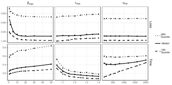
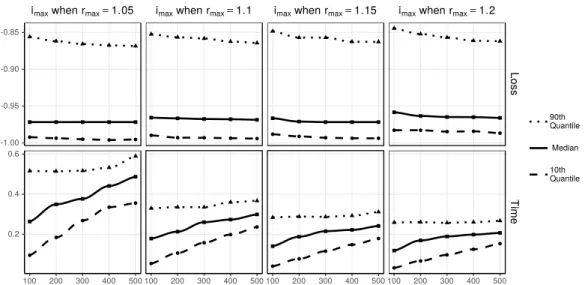
3.2.3 Approximation Ratio . . . 21 3.3 Algorithm . . . 22 3.3.1 Initialisation . . . 22 3.3.2 Optimisation . . . 24 3.3.3 Complexity . . . 25 4 Experiments 27 4.1 Parameters . . . 29 4.1.1 Initialisation . . . 29 4.1.2 Iterations . . . 31 4.1.3 Summary . . . 33 4.2 Robust Regression . . . 33 4.2.1 Scalability . . . 34 4.2.2 Robustness . . . 35 4.2.3 Optimality . . . 36 4.3 Explanations . . . 37 4.3.1 Classification of Text . . . 38 4.3.2 Classification of Images . . . 39

4.3.3 Classification of Particle Jets . . . 45

5 Conclusion 47 5.1 Weaknesses and Mitigations . . . 47

5.2 Future Work . . . 48 5.3 Open Source . . . 49 6 Sammanfattning 50 6.1 Robust regression . . . 50 6.2 Förklaringar . . . 51 6.3 Algoritm . . . 52 6.4 Experiment . . . 52 6.5 Slutsatser . . . 53 7 Bibliography 54

(6)

Abbreviations

Anchors Local explanations based on rules [50] (Explainer) C-Steps Concentration steps [54] (Optimisation)

CNN Convolutional Neural Network (Classifier)

EMNIST Extended MNIST [15]: Dataset of handwritten letters (Dataset) F1-Score Measure of classification quality (Evaluation)

Fast-LTS Faster _lts [54] (Robust Regression)

FCGI Finnish Grid and Cloud Infrastructure [22] (Computer Cluster) GDPR General Data Protection Regulation [3] (EU Regulation) IMDB Internet Movie DataBase [41] (Dataset)

L1-Norm Sum of absolute values, ∥x∥₁ =∑

i|xi| (Regularisation) L2-Norm Sum of squared values, ∥x∥₂ =∑

ix2i (Regularisation) LAD Least Absolute Deviation (Regression)

LAD-LASSO _lad with _lasso regularisation [66] (Regression) LASSO Least Absolute Shrinkage and Selection Operator [62]

(Regularisation)

LIME Local Interpretable Model-agnostic Explanations [49] (Explainer) LORE LOcal Rule-based Explanations [27] (Explainer)

LR Logistic Regression (Classifier)

LTS Least Trimmed Squares [52] (Robust Regression)

(7)

MES Model Explanation System [63] (Explainer) MM-Estimator Robust _m-estimator [67] (Robust Regression) MM-LASSO _mm-estimator with _lasso regularisation [59]

(Robust Regression)

MNIST Dataset of handwritten digits [36] (Dataset) NN Neural Network (Classifier)

OLS Ordinary Least-Squares (Regression)

Quasi-Newton Approximation of the Newton method (Optimisation) S-Estimator Robust estimates of scales [51] (Robust Regression) SHAP SHapley Additive exPlanations [40] (Explainer)

SLISE Sparse LInear Subset Explanations [9] (Robust Regression) Sparse-LTS _fast-lts with _lasso regularisation [4] (Robust Regression) SVM Support Vector Machine [16] (Classifier)

(8)

1. Introduction

Practically all real-world datasets contain outliers, items that do not adhere to the same structure as the rest of the data. These outliers are problematic when modelling or analysing the data, since even a single outlier can have a large negative impact on the outcome [32]. It is thus important to use methods that are robust to outliers. In this thesis I present a novel robust regression method termed _slise, Sparse LInear Subset Explanations. Specifically, _slise finds the largest subset of data items that can be represented by a linear model to a given accuracy.

Modern datasets tend to be quite large, both in terms of the number of items and in the number of variables. Efficient algorithms are crucial, espe-cially for interactive use, and _slise is able to outperform many of the existing robust regression methods on large datasets (shown in Section 4.2). Having many variables not only affects the running time, but also the interpretabil-ity. Sparse models (models where some of the coefficients are zero) are easier to interpret since the zero-coefficients can be ignored [38]. _slise uses _lasso regularisation [62] to produce sparse models.

Another feature of modern data science is the increased use of black box models, such as neural networks. These kinds of models are used since they can handle more complex data and thus provide better predictions. The downside is that the inner workings of black box models are often incomprehensible. Thus there is a growing need of explanations for what the models are doing. The Explanation part of the the name _slise comes from that one of the most interesting applications of _sliseis to explain outcomes from black box models. Existing explanation methods usually aim for either explaining everything the black box model might do (a global explanation, i.e., turn it into a trans-parent model) or just explaining individual decisions (local explanations). The explanations provided by _sliseare local and _slise does not require any mod-ifications to the black box models for it to work.

(9)

explained and then fitting a simpler model to this “neighbourhood”. The simple model approximates the black box model (locally) and is presented as the explanation. _slise does not require the user to design “reasonable” data-perturbations, but instead uses real data to fit the simple model. Specifically, slisefindsthe largest subset of data items that can be approximated by a linear model centred on a selected item. This has the added benefit that the subset can be used to measure how widely applicable the same explanation is to different items.

1.1 Disclosure

This thesis is based on a paper [9] where the _slise algorithm was introduced for the first time. I am the first author of that paper and have contributed to all parts of both the paper and the algorithm. This includes the design, the implementation, and the writing. This thesis is a new and stand-alone text but it shares some content with the paper, namely some definitions, some proofs, and some experimental results.

Compared to the paper [9] this thesis contains more theory and related works for the two main domains, robust regression and opaque model expla-nations. The thesis also includes improvements to the algorithm in the form of more proofs and different initialisation alternatives (of at least one is more robust). Furthermore the thesis extends the experiments with new parameter experiments and more ways of utilising explanations.

1.2 Contributions and Structure

This thesis presents a novel robust regression method, _slise, that can be used for explaining black box decisions. The problem _slisesolves can be described as finding the largest subset of data items that can be represented by a linear model to a given accuracy. This problem is NP-hard but _slise is able to solve it with a constant approximation ratio. Empiric evaluations on both real and synthetic datasets show that _sliseoutperforms some state-of-the-art robust regression methods. Furthermore _slise provides sensible explanations for black box models and extends existing explanation methods primarily in the use of real data instead of mutations.

(10)

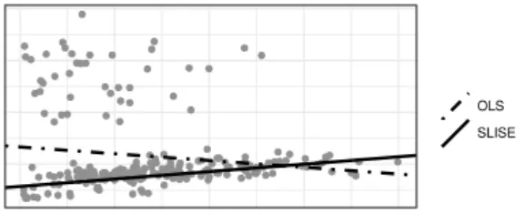
OLS SLISE

Figure 1.1: Robust regression example. The outliers in the upper left corner causes _olsregression to find a suboptimal model while_slise is able to ignore the outliers.

The introductory Chapter 1 gives a quick overview of the method and the two primary domains. The introduction concludes with two example scenar-ios where _slise can be used. Chapter 2 introduces the background for these two domains and discusses related works for both. The formal definition of the problem follows in Chapter 3 together with the proof that the problem is NP-hard. The same chapter also presents the algorithm and the numeri-cal approximations required by the algorithm. _slise is evaluated empirically in Chapter 4, using both synthetic and real-world datasets. The goal of the experiments is threefold, to select optimal parameters, to compare _slise to other robust regression methods, and to show how _slise can be used for ex-planations. This thesis ends with conclusions in Chapter 5 and a summary in Swedish in Chapter 6.

1.3 Examples

Next follows two simple examples of using_slise in the two domains. This not only demonstrates the usefulness of _slisebut also introduces some topics that will be expanded upon in the following chapters.

Robust Regression Figure 1.1 shows a two-dimensional dataset with outliers in the top-left. These outliers causes ordinary least-squares (_ols) regression to give a model that is a bad fit for most of the points. _slise, on the other hand, is largely unaffected by the outliers, by ignoring them, and finds a model that fits a large subset of the data.

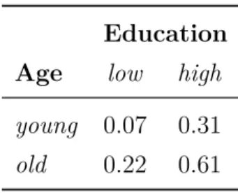
Explaining Black Box Models Table 1.1 shows the probabilities for having a high income, in a toy dataset, according to a simple classifier. Assume that the dataset consists of mostly people with a high education, for example, a faculty

(11)

Education

Age low high

young 0.07 0.31 old 0.22 0.61

Table 1.1: Explanation example. Probabilities of having a high income ac-cording to a simple classifier.

of a university department. A local explanation task could be to determine which factor is more important, age or education, for the classification of an old professor according to the classifier.

Looking at only the class probabilities in Table 1.1 it appears that education is more important, and this is indeed the explanation, e.g., the state-of-the-art local explanation method _lime [49] finds. However, knowing the education level for this person actually gives little information about the class since the dataset contains almost only people with high education. Instead, in this dataset, age is a better determinant of high income for the old professor, and this is what _slise returns.

The model in Table 1.1 is actually a simple logistic regression1_.

limefinds the largest coefficient in the logistic regression model, whereas _slisefinds the behaviour of the model in the dataset. The interaction between the model and the data is thus important, but can make the interpretation of even simple models non-trivial if the data has complex structures.

This insight is significant because it suggests that one cannot always cleanly separate the model from the data. An example of this is conservation laws in physical systems. If the data is accurate then the observations will never vio-late such laws and the model has no incentive to learn structures outside the constraints. Thus predictions for data breaking the constraints must be con-sidered either undefined or random. One may therefore find explanations that violate the laws of physics if the explanation method does not adhere to the constraints, or the data. _slise satisfies these kinds of constraints automati-cally, because the explanations are based on observing how the model behaves in the dataset, instead of randomly sampling (possibly non-physical) points around the item of interest (as in, e.g., [49, 50, 40, 27]).

1_{Probability of high income is given by}_p₌_σ₍₋₂_._{53 + 1}_.₇₃_·_{education + 1}_.₂₆_·_age),

(12)

2. Background

As described in the introduction _slise is a sparse robust regression method with applicability to explain decisions made by black box models. The next chapter contains the in-depth definition of _slise, while this chapter focuses on the theory of those two fields, as well as related methods for both.

2.1 Robust Regression

Normal regression is concerned with finding the relationship between one or more independent variables and one dependent variable. There are many ways to accomplish this, but one of the most basic methods isordinary least squares regression (_ols). _ols regression finds a linear model by minimising the sum of squared residuals. However it is very common for datasets to have samples with divergent values, called outliers. The reason these outliers exists can be anything from measurement errors to structures in the data that the regression model cannot describe. By squaring the residuals _olsgives a lot of weight to the outliers, which will affect the final model.

Robust regression methods are regression methods where the presence of outliers does not affect the results (too much) [53]. This means robust regres-sors minimise the effects the outliers have on the final model. The example in Figure 1.1 from the previous chapter shows a clear difference between robust and non-robust regression. _ols regression is not robust and thus the outliers have a large impact on the final model. There are multiple possible ways of accomplishing robustness, but normally the outliers are either de-emphasised or outright ignored. How the outliers are detected also differs between robust regression methods.

A popular measure of robustness is thebreakdown value[32] which measures how many of the samples in a dataset must be replaced by outliers in order to cause an arbitrarily large change in the model. For _olsregression a single

(13)

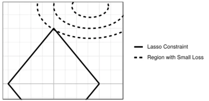
Lasso Constraint Region with Small Loss

Figure 2.1: Geometric interpretation of Lasso

outlier is enough to cause an arbitrarily large change, which corresponds to a breakdown value of 1/n, where n is the number of samples [32]. The best possible breakdown value is 1, but that implies that the model is independent of the data, which is not very useful. In practise the best breakdown value is 0.5, since if more than half of the data is replaced then the there is no way of telling which subset is the original one. But methods with smaller breakdown values may also perform well if the data does not contain a lot of outliers.

2.1.1 Sparsity

Another feature of some regression methods, including _slise, is the ability to produce sparse models. Sparse models are models with some of the coefficients being zero. This is especially useful for large datasets with many variables. The sparsity makes the models more interpretable, since sparsity helps you focus your attention on the variables that matter (those with coefficients other than zero).

Sparsity is often accomplished using a L1-norm on the model coefficients (∥α∥₁ = ∑

i|αi|), which is also known as lasso regularisation [62]. lasso (Least Absolute Shrinkage and Selection Operator) regularisation can either be used as a constraint ∥α∥₁ ≤ t or by adding it to a loss function with a Lagrange multiplier λ∥α∥₁. Here α is a vector that contains the coefficients for the regression model and t, λ≥0 are regularisation parameters.

The easiest way to show how_lasso regularisation produces sparse models is through a geometric interpretation, shown in Figure 2.1. The square repre-sents the allowed area where ∥α∥ ≤t and if the optimal non-sparse solution is outside the constraint then the boundary of the low-loss region, exemplified by the dashed-lines, is more likely to tangent the corners (sparse solutions) than the sides [62]. This is in contrast to using a L2-norm (Tikhonov regularisation

(14)

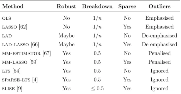
Method Robust Breakdown Sparse Outliers

ols No 1/n No Emphasised

lasso[62] No 1/n Yes Emphasised

lad Maybe 1/n No De-emphasised

lad-lasso [66] Maybe 1/n Yes De-emphasised mm-estimator[67] Yes 0.5 No Penalised

mm-lasso[59] Yes 0.5 Yes Penalised

lts[54] Yes 0.5 No Ignored

sparse-lts[4] Yes 0.5 Yes Ignored

slise[9] Yes ≤0.5 Yes Ignored

Table 2.1: Summary of some related robust regression methods

/ Ridge regression) where the boundary ∥α∥₂ ≤ t is a circle and no point is more likely to tangent than the rest.

2.1.2 Related Methods

Below follows descriptions for a couple of robust regression methods. They are selected to be well known, but also representative of different ways of handling outliers. The discussion naturally includes their breakdown value and mentions variants which include _lasso regularisation in order to provide sparsity. Table 2.1 shows a quick overview of some related methods (_ols, lasso and slise included for comparison). For a more in-depth survey see, e.g., [53, 59].

Least Absolute Deviation Least Absolute Deviation (_lad) is very similar to ordinary least squares but replaces the sum of squared residuals with a sum of absolute residuals. By not squaring the errors _lad is in practise more robust, which can be seen in, e.g., the robustness experiment in Section 4.2.2. But _lad has the same breakdown value as _ols (1/n) so it is not robust in a general case (also shown in Section 4.2.2). Using absolute values introduces two complications. The solutions are not unique and _lad cannot be solved analytically [2]. There are, however, multiple efficient iterative methods for solving _lad, e.g., [56, 8].

Similarly to how_olsregression can be extended with_lassoregularisation to create _lasso[62] (from where the name origins), _lasso regularisation can

(15)

also be added to _lad to create the sparse _lad-lasso algorithm [66].

MM-Estimator One of the earliest attempts at creating a robust regression algorithm is the_m-estimator which avoids outliers based on maximum like-lihood estimates. However, it was soon discovered that it has as low a break-down value as _ols, which suggests that in theory it is not robust [31]. This lead to the development of the _s-estimator[51] where the residual scales are robustly estimated (with similar calculations to the ones in_m-estimator). s-estimatoris a robust regression algorithm with a breakdown value of 0.5, but it is inefficient [67]. There are many other proposed alternative_m-estimators that address the robustness, some even quite recent ones [39, 11], but the most well known is _mm-estimator [67]. By using ideas from _s-estimator for initialisation _mm-estimator achieves the same breakdown value of 0.5, but still keeps the efficiency of _m-estimator.

The application of _lasso regularisation to create sparse variants of algo-rithms is something that continues with _mm-estimator, resulting in mm-lasso [59].

Least Trimmed Squares Least Trimmed Squares [52] (_lts) takes a different ap-proach by working with a subsetS, of a given size|S|=k wheren/2< k≤n. ltsfinds the linear model with the least sum of squared residuals forksamples (the subset), the rest n−k samples are ignored. Since _lts considers a subset of included items, rather than smoothly penalising outliers, it is a combina-torial problem. _lts has no closed-form solution, but algorithms provide good approximations. Another problem with (early) _lts was that the approxima-tion was inefficient, but that was solved with the development of the_fast-lts variant [54].

fast-lts starts from a number of candidate subsets then iteratively im-proves them with concentration steps (C-steps). For each step and candidate a linear model is calculated for the subset using _ols, then the subset is updated to contain the k samples with the least residuals. This procedure is guaran-teed to converge since the candidates either remain the same or are improved. When all candidates have converged (stopped improving) the best model is selected.

fast-lts has also been further enhanced with sparsity by the addition of lasso regularisation to create sparse-lts[4].

(16)

2.2 Explaining Classifiers

A surprising application of _sliseis in the field of explaining black box models. The phrase black box usually refers to machine learning models that are so complex that it is infeasible to understand their inner workings. But it could just as well be human experts refusing to offer motivations for their decisions. This section focuses on answering why you would need explanation, what ques-tions these explanaques-tions answer, and how a couple of existing methods work. For a more detailed review see, e.g., [28, 45].

2.2.1 The Need for Explanations

The most obvious reason for explanations is to build trust. The name black box in itself suggest that there is some opaque process going on, so one way to increase trust is to give insight into what is happening. While trust and understanding is important in general it is especially important in safety crit-ical applications, such as in medicine [10]. Beside building trust there are also some practical reasons for needing explanations.

The European Union recently enacted the General Data Protection Regu-lation (_GDPR [3]) which among other things stipulates the right for citizens to get an explanation for algorithmic decisions [26]. This is not limited to black box models, but obviously also covers them. The aim of this require-ment is not only to increase transparency but also to avoid systematic biases and discrimination. Discrimination is a known problem in machine learning [37] and has real consequences, e.g., Amazon did not deploy a new hiring tool after it showed signs of discrimination [17]. Methods exists for mitigating dis-crimination [29], but explanations can play a key role in detecting such biases [28, 49].

One popular type of black box models, deep learning, has been shown to outperform humans on tasks normally requiring expert knowledge, e.g., in lung cancer detection [19]. At the same time some established deep learning models have been shown to be fragile, where imperceptible changes to the input can cause drastically different results [60, 46, 25]. This would motivate a hybrid approach with both a trained model and a human expert. This has been successfully used in, e.g., [65, 42] where the breast cancer detection accuracy increased from 92.5 % to 99.5 % by introducing a human expert. For the

(17)

Interpretation

Globally Global Global

Interpretable Post-hoc Model Model Explanation Inspection

Locally Local Local

Lo

calit

y

Interpretable Post-hoc Model Model Explanation Inspection Table 2.2: Explanation categories

hybrid approach to work the model has to share more information than just the prediction. An explanation would naturally constitute such additional information.

A black box that is able to give accurate predictions probably has some internal representation of the data. Being able to extract that information could help with verifying that what the models is doing is reasonable. Fur-thermore, if the data is not fully understood then this information could be used to extend human knowledge. Both of these phenomena could be really beneficial in, e.g., scientific use-cases, such as when classifying particle-jets in high energy physics [18, 33].

2.2.2 Types of Explanations

Explanation of opaque models is currently a hot research topic, so naturally there are a lot of different approaches [28], but they can generally be categorised based on what they are trying to explain and the scope of the explanations. The categories are summarised in Table 2.2.

A natural start is to not create black boxes in the first place, and instead use simpler, interpretable models. Examples of interpretable models would be all kinds of simple models, such as decision trees and various nearest neighbours algorithms, but also some more advanced, e.g., Super-sparse Linear Integer Models [64], and Interpretable Decision Sets [34]. The big drawback with interpretable models is the same as the reason why we use black boxes; complex models can solve some (complex) problems better than interpretable models, and some problems are not at all solvable with current interpretable models.

If you do not want to sacrifice accuracy by simplifying the model then the next option is to use complex models and try to create explanations for the

(18)

outcomes after training. Contrary to the interpretable models above these explanations usually do not fit all data (global explanation), but rather focus on a single outcome (local explanation) [49, 28]. Not requiring an explanation for the whole black box might seem like a big limitation, but in many situation it is actually the preferred problem to solve. Compare listing all the things that might lead to cancer to listing the specific risk factors for a certain patient, if you were that patient then you would most likely be more interested in your personal factors, i.e., the local explanation.

Note that the explanation example from Section 1.3 uses a globally inter-pretable model (logistic regression). But due to structures in the data the variable with most weight in the global model was not the most important one in all local cases. Thus local explanations are still valuable even if you have a simple global model, especially if the local explanations are able to account for structures in the data.

Post-hoc local explanations are usually created by either finding a saliency map showing the important features or by approximating the complex model with an interpretable one [28]. The disadvantage with post-hoc explanations is that they are approximations (also applies to saliency maps), and the explana-tions can only be as good and expressive as the approximaexplana-tions. Furthermore when fitting approximations you often need a “neighbourhood” in which the approximation is valid, and defining this “neighbourhood” is not trivial [45, 27]. It is possible to create explanations for black boxes without using approx-imations, but they will naturally have more limited scope than any of the ap-proaches above. Instead of explaining the outcomes model inspection focuses on specific subprocedures of the black box (local or global). For example, Sen-sitivity Analysis measures how sensitive the outcome is to changes in the input variables [28], while Activation Maximisation [21] shows what kind of images would maximally activate specific layers in a convolutional neural network. For a survey of different ways of visualising layers in a convolutional neural network see, e.g., [48].

This brings in a third dimension for the categories [28] (not shown in Ta-ble 2.2); are the explanations model agnostic or model aware? Model agnostic explanation methods can be used on any black box, even humans, while model aware explanation methods uses some feature tied to specific types of models, e.g., neural networks offer gradients while random forests do not. Interpretable models can all be considered model aware (since the model is the explanation), but there exists both agnostic and aware methods for post-hoc explanations

(19)

and inspections. Explanation methods can also be be specialised on differ-ent kinds of data, but that is largely independdiffer-ent of the categories mdiffer-entioned previously.

2.2.3 Interpretability

All of the categories mentioned in the previous section have the same goal, transferring insights about the black box to a human. This requires the results to be interpretable. It is impossible to give an exact definition of interpretabil-ity, since it is subjective [38]. Generally a model is considered interpretable if it is simple and small [28, 38], e.g., linear models is easier to interpret than neural networks but a linear model with thousands of coefficients is usually not interpretable. The exact level of simplicity and size obviously depends on the persons doing the interpretation and their expertise [24]. This makes comparisons between model-families difficult.

Transparency is often used as a synonym to interpretability, and while these two concepts are not exactly the same thing, transparency can give additional tools for concretising interpretability. Transparency consists of three concepts; simulatability, decomposability, and algorithmic transparency [38]. Simulatability refers to the ability for a human to apply a model without the help of a computer, e.g., follow a decision tree. Decomposability states that all components, e.g., variables and calculations, should have a natural description and a reason for being used. Finally, Algorithmic Transparency extends the transparency to the training of the model [38]. Intuitively, using a black box model to create (transparent) explanations for another black box model creates distrust. Algorithmic transparency is this intuition quantified as a requirement.

Furthermore, the authors of [24, 38] note that the presentation also has an impact on the interpretability and that the correct choice of presentation depends on the context. However interpretability is not only about making the transfer of information easy, but sometimes also about maximising the amount of information transferred. For example, an expert might not trust too simple explanations [35]. It is also important to consider how the explanations will affect the behaviour of the humans seeing them. Seemingly good explanations will raise the trust in the model, even if it is misplaced. This can lead to more errors, such as obvious misclassifications, not being detected [47].

(20)

couple of high-level properties that explanations preferably should have can be found in, e.g., [28, 23, 38, 49]. Satisfying all of them at the same time might not be possible, and selecting the best trade-off depends on the situation.

Interpretability Keeping in mind the discussion above about the difficulty of measuring the interpretability, the target audience should at least be able to interpret the explanations.

Accuracy/Fidelity The explanations should match the black box. In the case of interpretable models this means fitting the data, while approximations should imitate the black box model. Both cases can be measured with standard accuracy measures, e.g., F1-scores.

Informativeness The explanations should give as much information as possi-ble, with the given representation. This definition is kept vague on purpose since it depends on the interpreters skills and because this might contradict the interpretability.

Stability/Generality Explaining similar samples should usually lead to similar explanations. Furthermore local approximations should be applicable to more samples than just the one being explained.

2.2.4 Related Methods

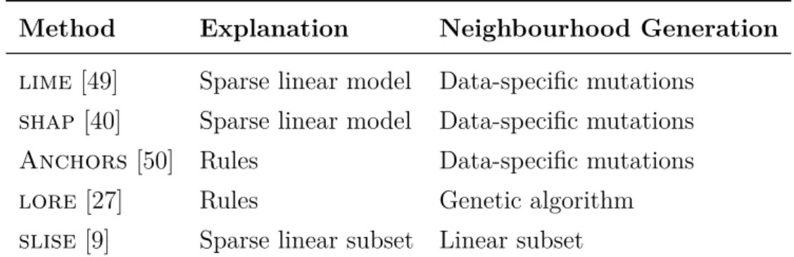
Following the categories outlined Section 2.2.2, _slise creates model-agnostic, local, post-hoc explanations. Thus all the related methods presented in this section are from this niche. A quick summary of the methods can be seen in Table 2.3. For a more complete review of explanations, including methods from other categories, see, e.g., [28, 45].

LIME Local Interpretable Model-agnostic Explanations [49]. _lime creates a neighbourhood by mutating the sample to be explained. The mutation is de-pendent on the data-type, e.g., images are mutated by grouping similar pixels into “super-pixels” (dimensionality reduction) and randomly replacing individ-ual super-pixels with a neutral colour (grey). Then all mutations are evaluated by the black box model and weighted according to the distance to the selected sample. Finally_limefits a weighted sparse linear model to the neighbourhood.

(21)

Method Explanation Neighbourhood Generation

lime [49] Sparse linear model Data-specific mutations shap [40] Sparse linear model Data-specific mutations Anchors[50] Rules Data-specific mutations

lore [27] Rules Genetic algorithm

slise [9] Sparse linear subset Linear subset

Table 2.3: Summary of some related model-agnostic, local, post-hoc explana-tion methods

Intuitively, changing the features the model uses for classification will cause a change in the prediction, which _lime utilises in the explanation.

SHAP SHapleyAdditive exPlanations [40]. _shapgeneralises_limeand a couple of other [7, 58]additive feature attribution methods. _shapextends the previous works by setting parameters based on theoretical Shapley values, rather than heuristically. This leads to more stable and accurate explanations.

Anchors _Anchors[50] addresses two of the issues with_lime; a linear model is not suitable for all kinds of models and it is unclear if the explanations are applicable to other samples than the one being explained. The name, An-chors, refers to the explanations that are in the form of rules constructed such that almost all samples for which the rules hold have the same classifica-tion. In the creation of the rules _Anchorsuses a similar mutation process to the mutations in _lime.

LORE LOcal Rule-based Explanations [27]. The authors of _lore criticise lime, and similar methods, for having very uncontrolled mutations. loreuses a genetic algorithm for controlling the mutations, mostly by penalising muta-tions far away from the explained sample according to a normalised Euclidean distance measure. This has the added advantage of letting_lore present coun-terfactuals, i.e., the minimum alternation needed to change the classification.

Other The methods above is just a sample of local, model-agnostic, post-hoc explainers and, e.g., _mes [63] could replace _Anchors since both give explanations in the form of rules, but with different algorithms for finding the rules. Furthermore by not requiring the methods to be model-agnostic there are more features that the explainers can use, such as when [23] uses

(22)

gradients from a neural network to find good perturbations of the data item being explained. Finally the authors of [30] states that one needs to be careful when interpreting linear models. This is especially important for users that are not familiar with inference, since the model coefficients show how the model uses the data to infer the outcome and not which (latent) features are important for the outcome. [30] further offers a way of using the linear model to find the important latent features.

(23)

3. The SLISE Algorithm

slise is a robust linear regression method that findsthe largest subset of data items that can be represented by a linear model to a given accuracy. The solution to this problem has applications to bothglobal robust linear regression and local linear regression that approximates the decision surface of a black box model in the vicinity of a data item. The problem is formally defined in Section 3.1.

Of the existing robust regression methods _slise is most closely related to lts, and its variants. Both utilise a subset and derive their robustness from ignoring outliers. However, there is a major difference; in _lts the size of the subset is fixed a priori while in _slise the size is dynamic. This breaks the assumptions needed for the _fast-lts algorithm and thus a novel algorithm (_slise) is developed in Section 3.2 and 3.3.

3.1 Problem Definition

Let (X ∈ _Rn×d_{, Y} _∈

Rn) be a dataset that consists of n pairs {(xi, yi)}ni=1, where xi (the predictor) denotes the ith d-dimensional item (row) in X and

yi (the response) denotes the ith element in Y. Furthermore let ε ≥0 be the largest tolerable error and λ≥0 be a regularisation coefficient. With this the main problem can now be stated:

Problem 3.1. Given X ∈_Rn×d_, _Y _∈

Rn, and non-negative ε, λ∈R, find the

regression coefficients α∈_Rd _{minimising the loss function} Loss(X, Y, ε, λ, α) =∑n

i=1H

(

ε2−r2_i) (r_i2/n−ε2)+λ∥α∥₁, (3.1) where the residual errors are given by ri = yi −α⊺xi, H(·) is the Heaviside step function satisfying H(u) = 1 if u ≥ 0 and H(u) = 0 otherwise, and ∥α∥₁ = ∑d

i=1|αi| denotes the L1-norm. If necessary, the data matrix X has been augmented with a column of all ones to accommodate the intercept term of the model.

(24)

Note that this is a combinatorial problem in disguise where we try to find the largest possible subset S. Using the short form [n] = {1, . . . , n} Equa-tion 3.1 can be rewritten, in combinatorial form, as

Loss(X, Y, ε, λ, α) =∑ i∈S

(

r_i2/n−ε2)+λ∥α∥₁ whereS ={i∈[n]|r2_i ≤ε2}.

(3.2) The loss function of Equation 3.1 (and Equation 3.2) thus consists of three parts; the maximisation of subset size∑

i∈Sε2 =|S|ε2, the minimisation of the residuals ∑

i∈Sri2/n≤ε2, and the lasso-regularisation λ∥α∥1. The main goal is to maximise the subset and this is reflected in the loss function, since any decrease of the subset size has an equal or greater impact on the loss than all the residuals combined. At the limit of ε → ∞ it follows that S = [n] and Problem 3.1 becomes equivalent to _lasso [62].

3.1.1 Breakdown Value

In the beginning of this chapter it is mentioned that Problem 3.1 requires a new algorithm, but it also requires a new proof for the breakdown value.

Theorem 3.1. The breakdown value of _slise is |S0|/(2n)≤0.5, where S0 is the subset given by slise when the dataset contains no outliers.

Proof. Following the definition from [32, 53, 20] the breakdown value can be found by starting with a uncorrupted dataset (X0, Y0) with no outliers and then adversarially change the values of a fraction v of the data items into adversarial values. The breakdown value is the minimum v that can cause an arbitrarily large deviation in the model.

The subset given by _slise on (X0, Y0) is S0 and on the corrupted dataset (Xv, Yv) the subset is Sv. slise breaks down when Sv consists of corrupted items (|Sv|/n = v). This can happen when |Sv| ≥ |S0 \ Sv|.1 Rearranging yields v ≥ |S0\Sv|/n≥ |S0|/2/n.

The breakdown value for _slise is thus dependent on the data. If, for example, the second largest (independent) linear subset is larger than |S0|/2 then the_slisebreaks down withv >|S0|/(2n). However the breakdown value is a measure of worst case, so the theorem still holds. _sliseachieves the largest possible data-dependent breakdown value if the relation between X0 and Y0

1_S

(25)

is linear (within an error tolerance of ε). Then |S0| =n and the breakdown value becomes 0.5, which is the practical upper limit for robustness.

3.1.2 Explaining Classifiers

Local explanations require the model to be local to the data item being ex-plained, (xk, yk) where k ∈ [n]. This can be accomplished with slise by adding an additional constraint to Problem 3.1, requiring that the linear model passes through this item, i.e., yk −α⊺xk = rk = 0. Centring the data on this item by using yi → yi − yk and xi → xi − xk for all i ∈ [n] causes

rk = (yk−yk)−α⊺(xk−xk) = 0, which fulfils the constraint. Note that this also eliminates any potential intercept by setting it to zero. Hence it is suf-ficient to only consider Problem 3.1 for both finding global regression models (robust regression) and local regression models (local explanations).

As noted in Section 3.1.1 _slise works best if the relation between X and

Y is close to linear. Thus, in practise, if a classifier outputs class probabilities

P ∈[0.0,1.0]n we transform them into linear values using a logit transforma-tion, yi = log(pi/(1−pi)), for all i ∈[n]. This yields the vector Y ∈ Rn that is used with_slise (or Y −yk in the case of local explanations). Note that this linear model is comparable to the linear model obtained using normal logistic regression.

The explanations offered by_slisethus consist of a linear/logistic regression that approximates the black box model around the outcome being explained (xk, yk). This is comparable to many of the other local explanation methods described in Section 2.2.4. Additionally, _slise also offers a subset of the data items where the approximation is valid, allowing for an error of maximally ε. Further details and examples of explanations are given in Section 4.3.

3.1.3 Complexity

An algorithm approximating Problem 3.1 is developed in the following sections. The approximation is needed when the number of items grows beyond a trivial amount due to the complexity of Problem 3.1.

Theorem 3.2. Problem 3.1 is NP-hard and hard to approximate.

Proof. This can be proven by a reduction to the _{maximum satisfying} lin-ear subsystemproblem [6, Problem MP10], which is known to beNP-hard.

(26)

The _{maximum satisfying linear subsystem}problem is defined as finding

α ∈_Qd _{such that as many equations as possible in}_Xα₌_y_{are satisfied, where}

X ∈_Zn×d_and_y_∈

Zn. This is equivalent to Problem 3.1 withε= 0 andλ= 0.

The _{maximum satisfying linear subsystem}problem is not approximable within nγ _{for some} _{γ >}_{0, according to [5].}

3.2 Numerical Optimisation

Since Problem 3.1 is NP-hard it has to, in practice, be solved approximately for all but trivial datasets. The combinatorial Problem 3.1 is relaxed into an optimisation problem by replacing the Heaviside function with a sigmoid function σ(x) = 1/(1 +e−x) and a rectifier function ϕ(u) ≈ min (0, u). This allows us to compute the gradient and find α by minimising

β-Loss(X, Y, ε, λ, α) =∑n i=1σ

(

β(ε2−r_i2))ϕ(r_i2/n−ε2)+λ∥α∥₁, (3.3) where the parameter β determines the steepness of the sigmoid. The rectifier function ϕ is required in order to ensure that large residuals (> nε2_{) do not} affect the loss, since the sigmoid function never gives zeroes for finite values. Furthermore the rectifier function needs to be continuous and differentiable, and is defined as ϕ(u) =uforu≤ −ω,ϕ(u) =−(u2_/ω₊_ω₎_/_{2 for}₋_{ω < u <}_0, and ϕ(u) =−ω/2 for 0≤u, where ω >0 is a small constant. Equation 3.3 is a smoothed variant of Equation 3.1 (in Problem 3.1) and becomes equivalent to Equation 3.1 when β → ∞and ω→0+_.

3.2.1 Graduated Optimisation

The minimisation of Equation 3.3 is done using graduated optimisation. The idea behind graduated optimisation is to iteratively solve a difficult optimisa-tion problem by progressively increasing the complexity [44]. A natural way to increase the complexity of Equation 3.3 is by gradually increasing the β

parameter. With β = 0 the problem is convex and equivalent to _lasso, while with β → ∞ it corresponds to Problem 3.1, which is NP-hard. At each step (of increasing β values) the previous value of α is used as a starting point for finding the new minimum of Equation 3.3.

It is important that consecutive solutions (with increasing β values) are close enough for graduated optimisation to work, which is why we derive an

(27)

approximation ratio between solutions with different values of β. The deriva-tion starts with the observaderiva-tion that the minimisaderiva-tion of Equaderiva-tion 3.3 can be rewritten as a maximisation of −β-Loss(X, Y, ε, λ, α). Furthermore the L1-regularisation term is unaffected by β and is omitted for simplicity.

Theorem 3.3. Given β1, β2 ≥0, such that β1 < β2, and the functions

fj(r) =−σ(βj(ε2−r2))ϕ(r2/n−ε2), and Gj(α) =∑ni=1fj(ri) where

ri =yi−α⊺xi and j ∈ {1,2}. The inequality G2(α2)≤KG2(α1) always holds where α1 = arg maxαG1(α), α2 = arg maxαG2(α), and

K =G1(α1)/(G2(α1) minrf1(r)/f2(r)) is the approximation ratio.

Proof. Let us first argue the non-negativity of f1 and f2. The inequalities

σ(u)>0 and ϕ(u)<0 hold for all u∈_R, thus fj(r)>0. Now, by definition,

G1(α2) ≤G1(α1). We denote r∗i =yi−α⊺2xi and k = minrf1(r)/f2(r), which allows us the rewrite and approximate:

G1(α2) = ∑n i=1f1(r ∗ i) = ∑n i=1f2(r ∗ i)f1(ri∗)/f2(r∗i)≥kG2(α2).

Then G2(α2) ≤ G1(α2)/k ≤ G1(α1)/k ≤ G2(α1)G1(α1)/(kG2(α1)), and the inequality from the theorem holds.

The approximation ratio K in Theorem 3.3 can be used to select the se-quence ofβvalues (β0 = 0, β1, β2. . .). At each step the nextβvalue is chosen so thatK stays within a bound specified by the parameterrmaxin Algorithm 3.1.

3.2.2 Stopping Criteria

Iterating until β → ∞ is not possible, so at some point the algorithm has to stop. The stop should trigger when σ(β(ε2₋_r2₎₎_≈_H₍_ε2₋_r2_{), i.e. the stop} is dependent on the shape of the sigmoid function. The shape is determined by both β and ε. However ε is expected to change regularly so a stopping shape that is independent of ε is needed.

The goal is to find a function for βmax that works with arbitrary values of

ε. Assume there exists a pair of valuesβopt andεopt that results in an optimal stopping shape for the sigmoid function. The two sigmoid functions have the same relative shape if and only ifσ(βmax(ε2−(pε)2)) =σ(βopt(ε2opt−(pεopt)2)) for every value of p ∈ _R. The sigmoid function is strictly increasing and can

(28)

trivially be removed from both sides

σ(βmax(ε2−(pε)2)) =σ(βopt(ε2opt−(pεopt)2))

βmaxε2(1−p2) = βoptε2opt(1−p2)

βmax=βoptε2opt/ε

2 ₌_c/ε2_,

(3.4)

wherec=βoptε2optis a constant. The actual value ofcis empirically determined in Section 4.1.2.

3.2.3 Approximation Ratio

Theorem 3.2 not only shows that Problem 3.1 is NP-hard, but also that it is hard to approximate. Using the approximation ratio between two β-Losses we derive a new approximation ratio between Equation 3.3 and Equation 3.1. To do that we set β2 → ∞ so that f2(r) = −H(ε2 −r2)(r2/n−ε2). Ad-ditionally we introduce an ε∗ such that f₂∗(r) = −H(ε∗2 −r2)(r2/n−ε∗2),

G∗₂(α) = ∑n

i=1f2∗(yi−α⊺xi), and α∗2 = arg minαG∗2(α). This leads to a new approximation ratio Kε∗:

Lemma 3.1. The approximation ratio between α1 and α∗2 is Kε∗ =

G1(α1)/(G∗2(α1)kε∗) where k_ε∗ =σ(β₁(ε2−ε∗2))ϕ(ε∗2/n−ε2)/(ε∗2/n−ε∗2).

Proof. The proof is omitted since it exactly mirrors Theorem 3.3 with the observation that kε∗ = min_rf₁(r)/f∗

2(r) = minr≤ε∗−f₁(r)/(r2/n−ε∗2) which

leads to kε∗ =σ(β₁(ε2−ε∗2))ϕ(ε∗2/n−ε2)/(ε∗2/n−ε∗2).

The first goal is to find a value ofε∗such that the approximation ratioKε∗is

minimised. This can be written as ε∗ = arg min_ε∗K_ε∗ = arg max_ε∗G∗₂(α₁)k_ε∗,

which leads to ε∗ = arg max ε∗ − n ∑ i=1 H(ε∗2−r_i2)(r_i2/n−ε∗2)σ(β1(ε 2₋_ε∗2₎₎ ϕ(ε∗2/n−ε2) ε∗2_/n₋_ε∗2 (3.5) where ri =yi−α⊺1xi. Thanks to the non-continuity of the Heaviside function the maximum can be found at ε∗ = rj for some j ∈ [n]. Furthermore, with a large large enough n, so that 1/n ≈ 0, Equation 3.5 can be simplified to

ε∗ ≈ arg max_r

j

∑n

i=1H(r2j −r2i)σ(β1(ε2 −rj2)). We can also assume, without a loss of generality, that the residuals are sorted so that r2

1 ≤ r22 ≤ . . . ≤ rn2, which means that ∑n

i=1H(rj2−r2i) = j and ε∗ ≈arg maxrjj·σ(β1(ε

2₋_r2 j)). We call α∗₂ (the optimum for Problem 3.1 with ε∗) the matching solution. If the data is subsampled to a constant size then Equation 3.3 has a constant approximation ratio for the matching solution.

(29)

Theorem 3.4. The matching solution satisfies the inequality

G∗₂(α∗₂)≤K∗G₂∗(α1) where K∗ =O(logn) is the approximation ratio. Proof. By definition Krt ≥ Kε∗ where t ∈ [n], Krt = G1(α1)/(−

∑n i=1H(r2t − r2 i)(ri2/n− r2t)krt), and krt = σ(β1(ε 2 ₋ _r2 t))ϕ(r2t/n−ε2)/(r2t/n −r2t). This is the same as in Lemma 3.1. Assuming the residuals are sorted so that

r₁2 ≤r2₂ ≤. . .≤r2_n (the same as above), Krt ≥Kε∗ can be rearranged as

σ(β1(ε−r2t))≤G ∗ 2(α1)kε∗/(− n ∑ i=1 H(r2_t −r_i2)(r_i2/n−r2_t)ϕ(r2_t/n−ε2)/(r2_t/n−r2_t)) ≤G∗₂(α1)kε∗/(−t(r2_t/n−r_t2)ϕ(r2_t/n−ε2)/(r_t2/n−r2_t)) =−G∗₂(α1)kε∗/(tϕ(r2 t/n−ε 2₎₎_. Inserting this into G1 yields

G1(α1) = − ∑n i=1σ(β1(ε 2₋_r2 i))ϕ(r 2 i/n−ε 2₎ ≤ −∑n i=1−G ∗ 2(α1)kε∗/(iϕ(r2_i/n−ε2))ϕ(r2_i/n−ε2) =G∗₂(α1)kε∗ ∑n i=11/i ≤G∗₂(α1)kε∗(logn+ 1).

And combined with Kε∗ from Lemma 3.1 this leads to Kε∗ =G₁(α₁)/(G∗

2(α1)kε∗)≤G∗

2(α1)kε∗(logn+1)/(G∗

2(α1)kε∗) = logn+1.

3.3 Algorithm

This section presents the algorithm, _slise, that approximately solves Prob-lem 3.1, using the approximations described above. Following the high-level pseudocode in Algorithm 3.1, _slise starts with selecting initial values for the linear modelαand the sigmoid steepnessβ(line 3). The second phase of _slise is the graduated optimisation (lines 4–7).

3.3.1 Initialisation

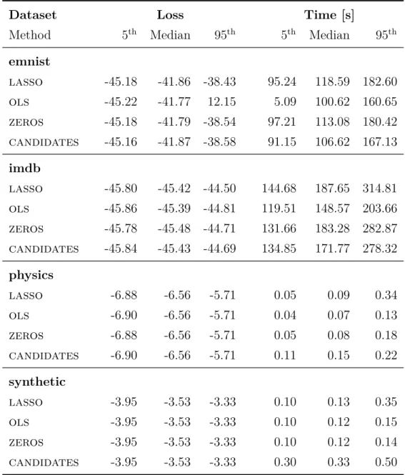
In total four alternative initialisation schemes are presented as pseudocode in Algorithm 3.2 and 3.3. These are later compared empirically in Section 4.1.1. The first initialisation alternative (Algorithm 3.2, lines 2–5) is to use _lasso -regression. _lasso-regression is the non-robust counterpart to _slise. It is also straight forward to implement since it only requires β = 0 (_lasso is a convex

(30)

1 Parameters: (1) Dataset X ∈_Rn×d,Y ∈_Rn,

(2) error tolerance ε,

(3) regularisation coefficient λ,

(4) maximum sigmoid steepness βmax, (5) target approximation ratio rmax 2 Function SLISE(X, Y, ε, λ, β_max, r_max)

3 α, β ←Initialise(X, Y, ε, r_max) 4 while β < β_max do

5 α← OWL-QN(β-Loss, X, Y, ε, λ, α)

6 β←β′ such that AppoximationRatio(X, Y, ε, β, β′, α) =rmax 7 α← OWL-QN(β-Loss, X, Y, ε, λ, α)

8 Result: α

Algorithm 3.1: The _slise algorithm.

problem so the initial α does not matter). However setting β = 0 removes all notion of a subset, which has a major impact on the loss function.

Withβ > 0 the problem is no longer convex and the choice of α becomes

important. The second initialisation scheme (Algorithm 3.2, lines 6–9) uses ols-regression to find α and the approximation ratio (Theorem 3.3) to select

β (further explained below). However neither _ols nor _lasso is robust. The third alternative (Algorithm 3.2, lines 10–13) is similar to the second, but uses a constant α instead. The constant α consists of only zeros, i.e. starting from a super-sparse solution. The β is also chosen based on the approximation ratio (Theorem 3.3).

The final alternative (Algorithm 3.3) is inspired by another robust regres-sion method, _fast-lts [54]. A number uinit of candidates are generated of which the best one is selected. The candidates are generated by drawing ran-dom subsets (XS, YS) and fitting linear models to them (using ols-regression, lines 6–7). The probability that at least one of the subsets is free from outliers is given by p = 1−(1−(1−o)d₎u_{, where} _o _{is the fraction of outliers,} _d _the number of dimensions, and u the number of candidates. If d is large then u

would also have to be large to compensate for the decreased probability. To alleviate this issue we create smaller subsets (line 9) and fit the model using pca (line 10) when d is large. The best candidate is the one that minimises the β-Loss (lines 11-14).

(31)

(3) target approximation ratio rmax 2 Function InitialiseLasso(X, Y)

3 α← OrdinaryLeastSquares(X, Y) 4 β ←0

5 Result: α, β

6 Function InitialiseOLS(X, Y, ε, rmax) 7 α← OrdinaryLeastSquares(X, Y)

8 β ←β′ such that AppoximationRatio(X, Y, ε, 0, β′, α) = r_max 9 Result: α, β

10 Function InitialiseZeros(X, Y, ε, rmax) 11 α←0

12 β ←β′ such that AppoximationRatio(X, Y, ε, 0, β′, α) = r_max 13 Result: α, β

Algorithm 3.2: Deterministic initialisation schemes.

3.3.2 Optimisation

With the initial values for α and β we now perform graduated optimisation, where we gradually increase the value ofβ until we reachβmax (Algorithm 3.1, lines 4–6). At each iteration we find the α that minimises the β-Loss from Equation 3.3 using the current value of β (line 5). This optimisation is done with _owl-qn [57] which is a quasi-Newton optimisation method with built-in L1-regularisation. We then increase β (line 6) such that the approximation ratio K from Theorem 3.3 between the new and old β equals rmax. The ap-proximation ratio K is translated into code in Algorithm 3.4.

In Equation 3.3 we use the rectifier function ϕ to ensure negativity. This function requires a constant ω that we choose to have a magnitude less than the smallest positive value that can be expressed with a floating-point num-ber. This makes ϕ(u) numerically equivalent to min(0, u), which is used in Algorithm 3.4. A minor side-effect of this simplification is that lines 8–10 are needed to avoid division by zero (which would not happen with the proper ϕ).

(32)

(3) target approximation ratio rmax, (4) number of candidates uinit

2 Function InitialiseCandidates(X, Y, ε, r_max, u_init)

3 α, β, l←0,0,0 4 for i= 1, . . . , u_init do 5 if d≤12 then 6 X_S, Y_S ← RandomSubset(X, Y, size =d) 7 α′ ← OrdinaryLeastSquares(XS, YS) 8 else 9 X_S, Y_S ← RandomSubset(X, Y, size = 10) 10 α′ ← InversePCA(OrdinaryLeastSquares(PCA(X_S), Y_S)) 11 if β-Loss(X, Y, ε, 0, α′) < l then 12 α ←α′

13 β ←β′ such that AppoximationRatio(X,Y, ε,0,β′,α)=rmax 14 l ← β-Loss(X, Y, ε, 0, α)

15 Result: α, β

Algorithm 3.3: Non-deterministic initialisation scheme.

3.3.3 Complexity

The complexity of Algorithm 3.1 is different than the complexity of Prob-lem 3.1 and can be derived from pseudocode above. The initialisation has at most a complexity of O(nd2_u

init) which is less than the complexity of the optimisation. There are three main contributors to the complexity of the op-timisation; the loss function, _owl-qn, and the graduated optimisation. The evaluation of the loss function has a complexity of O(nd), due to the multi-plication between the linear model α and the data-matrix X. _owl-qn has a complexity of O(dpo), wherepo is the number of iterations. Graduated optimi-sation is also an iterative method O(pg), but it only adds the approximation ratio calculation, which is not dominantO(nd). Combining these complexities yields a complexity ofO(nd2p) for_slise, wherep=po+pg is the total number of iterations.

(33)

1 Parameters: (1) Dataset X ∈_Rn×d,Y ∈_Rn, (2) error tolerance ε, (3) sigmoid steepness β1,β2, (4) linear model α 2 Function AppoximationRatio(X, Y, ε, β₁, β₂, α) 3 f ← function(r, β) : −σ(β(ε2−r2)) 4 ϕ← function(r) : min(0, r2_/n₋_ε2₎ 5 k← minimize(f(r, β1)/f(r, β2), by adjusting r) 6 for i= 1, . . . , n do 7 r_i ←y_i−α⊺x_i 8 if ∑n_i₌₁ϕ(r_i) = 0 then 9 K ←∑n_i₌₁f(r_i, β₁)/(∑n_i₌₁f(r_i, β₂)·k) 10 else 11 K ←∑n_i₌₁f(r_i, β₁)ϕ(r_i)/(∑n_i₌₁f(r_i, β₂)ϕ(r_i)·k) 12 Result: K

(34)

4. Experiments

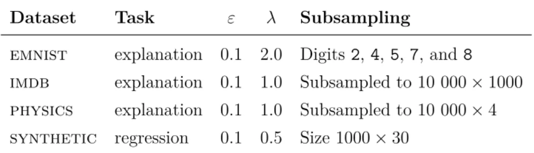
The experiments have three goals; find good default parameters, compare_slise to other robust regression methods, and show that _slise can produce reason-able explanations for black box models. This chapter is thus split into three parts corresponding to those goals. In Section 4.1 suitable default values for the parameters and a robust default initialisation method are determined em-pirically. Section 4.2 demonstrates that _slise is a robust regression method, that it scales to large datasets better than competing methods, and that it gives the best solution to Problem 3.1. Finally in Section 4.3 different ways of utilising _slise for explaining black box decisions are demonstrated, this also includes a brief comparison to another local explanation method.

slise and all the experiments are implemented in R [43] (version 3.5.1). The experiments were run on a high-performance cluster [22], where each job were allocated 4 cores from an Intel Xeon E5-2680 processor running at 2.4 GHz and 16 GB of RAM. The source code for _slise and all the experiments is released under an open source license and is available from

http://www.github.com/edahelsinki/slise.

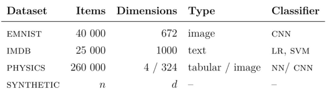
Datasets The experiments use a combination of real and synthetic datasets. The real datasets are handwritten digits (_emnist [15]), movie reviews (_imdb [41]), and particle jets (_physics, [1]). _synthetic datasets are used when specific dimensions are needed and are generated as follows. The data matrix

X ∈ _Rn×d _{is created by sampling from a normal distribution with zero mean} and unit variance. The response vector Y ∈ _Rn _{is created by} _y

i ← a⊺xi plus some normal noise with zero mean and 0.05 variance, where a ∈_Rd _{is one of} nine linear models drawn from a uniform distribution between−1 and 1. Each of the nine model creates 10% of the Y-values, except one that creates 20% of the Y-values. This larger chunk should enable robust regression methods to find the corresponding model. An overview of all the datasets is shown in Table 4.1.